Filter the data on excel

Try it!

Use filters to temporarily hide some of the data in a table, so you can focus on the data you want to see.

Filter a range of data

Select any cell within the range.
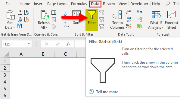
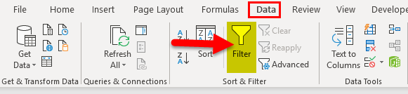
Select Data > Filter.
Select the column header arrow .
Select Text Filters or Number Filters, and then select a comparison, like Between.
Enter the filter criteria and select OK.

Filter data in a table

When you Create and format tables, filter controls are automatically added to the table headers.

Select the column header arrow for the column you want to filter.
Uncheck (Select All) and select the boxes you want to show.
Click OK.

The column header arrow changes to a Filter icon. Select this icon to change or clear the filter.

Want more?

Filter data in a range or table

Filter data in a PivotTable

Need more help?

Want more options?

Explore subscription benefits, browse training courses, learn how to secure your device, and more.

Communities help you ask and answer questions, give feedback, and hear from experts with rich knowledge.

Источник

Use AutoFilter or built-in comparison operators like «greater than» and “top 10” in Excel to show the data you want and hide the rest. Once you filter data in a range of cells or table, you can either reapply a filter to get up-to-date results, or clear a filter to redisplay all of the data.

Use filters to temporarily hide some of the data in a table, so you can focus on the data you want to see.

Filter a range of data

Select any cell within the range.
Select Data > Filter.
Select the column header arrow .
Select Text Filters or Number Filters, and then select a comparison, like Between.
Enter the filter criteria and select OK.

Filter data in a table

When you put your data in a table, filter controls are automatically added to the table headers.

Select the column header arrow for the column you want to filter.
Uncheck (Select All) and select the boxes you want to show.
Click OK.

The column header arrow changes to a Filter icon. Select this icon to change or clear the filter.

Filter data in a table

When you put your data in a table, filtering controls are added to the table headers automatically.

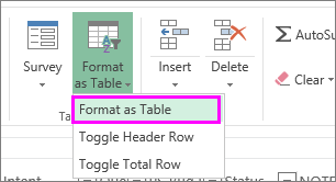
Select the data you want to filter. On the Home tab, click Format as Table, and then pick Format as Table.
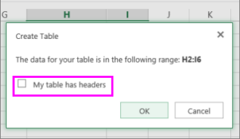
In the Create Table dialog box, you can choose whether your table has headers.
- Select My table has headers to turn the top row of your data into table headers. The data in this row won’t be filtered.
- Don’t select the check box if you want Excel for the web to add placeholder headers (that you can rename) above your table data.
Click OK.
To apply a filter, click the arrow in the column header, and pick a filter option.

Filter a range of data

If you don’t want to format your data as a table, you can also apply filters to a range of data.

Select the data you want to filter. For best results, the columns should have headings.
On the Data tab, choose Filter.

Filtering options for tables or ranges

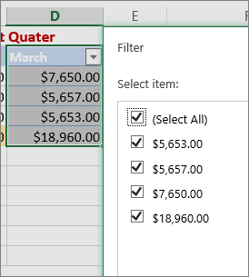
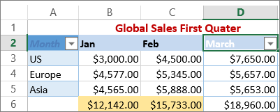
You can either apply a general Filter option or a custom filter specific to the data type. For example, when filtering numbers, you’ll see Number Filters, for dates you’ll see Date Filters, and for text you’ll see Text Filters. The general filter option lets you select the data you want to see from a list of existing data like this:

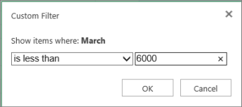
Number Filters lets you apply a custom filter:

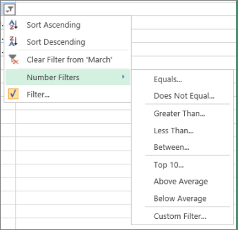
In this example, if you want to see the regions that had sales below $6,000 in March, you can apply a custom filter:

Here’s how:

Click the filter arrow next to March > Number Filters > Less Than and enter 6000.
Click OK.

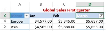
Excel for the web applies the filter and shows only the regions with sales below $6000.

You can apply custom Date Filters and Text Filters in a similar manner.

To clear a filter from a column

Click the Filter button next to the column heading, and then click Clear Filter from <«Column Name»>.

To remove all the filters from a table or range

Select any cell inside your table or range and, on the Data tab, click the Filter button.

This will remove the filters from all the columns in your table or range and show all your data.

Click a cell in the range or table that you want to filter.
On the Data tab, click Filter.
Click the arrow in the column that contains the content that you want to filter.
Under Filter, click Choose One, and then enter your filter criteria.

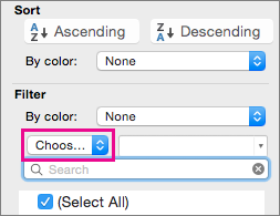
Notes:

You can apply filters to only one range of cells on a sheet at a time.
When you apply a filter to a column, the only filters available for other columns are the values visible in the currently filtered range.
Only the first 10,000 unique entries in a list appear in the filter window.

Click a cell in the range or table that you want to filter.
On the Data tab, click Filter.
Click the arrow in the column that contains the content that you want to filter.
Under Filter, click Choose One, and then enter your filter criteria.
In the box next to the pop-up menu, enter the number that you want to use.
Depending on your choice, you may be offered additional criteria to select:

Notes:

You can apply filters to only one range of cells on a sheet at a time.
When you apply a filter to a column, the only filters available for other columns are the values visible in the currently filtered range.
Only the first 10,000 unique entries in a list appear in the filter window.
Instead of filtering, you can use conditional formatting to make the top or bottom numbers stand out clearly in your data.

You can quickly filter data based on visual criteria, such as font color, cell color, or icon sets. And you can filter whether you have formatted cells, applied cell styles, or used conditional formatting.

In a range of cells or a table column, click a cell that contains the cell color, font color, or icon that you want to filter by.
On the Data tab, click Filter .
Click the arrow in the column that contains the content that you want to filter.
Under Filter, in the By color pop-up menu, select Cell Color, Font Color, or Cell Icon, and then click a color.

This option is available only if the column that you want to filter contains a blank cell.

Click a cell in the range or table that you want to filter.
On the Data toolbar, click Filter.
Click the arrow in the column that contains the content that you want to filter.
In the (Select All) area, scroll down and select the (Blanks) check box.
Notes:
- You can apply filters to only one range of cells on a sheet at a time.
- When you apply a filter to a column, the only filters available for other columns are the values visible in the currently filtered range.
- Only the first 10,000 unique entries in a list appear in the filter window.

Click a cell in the range or table that you want to filter.
On the Data tab, click Filter .
Click the arrow in the column that contains the content that you want to filter.

Under Filter, click Choose One, and then in the pop-up menu, do one of the following:

To filter the range for	Click
Rows that contain specific text	Contains or Equals.
Rows that do not contain specific text	Does Not Contain or Does Not Equal.

In the box next to the pop-up menu, enter the text that you want to use.

Depending on your choice, you may be offered additional criteria to select:

To	Click
Filter the table column or selection so that both criteria must be true	And.
Filter the table column or selection so that either or both criteria can be true	Or.

Click a cell in the range or table that you want to filter.
On the Data toolbar, click Filter .
Click the arrow in the column that contains the content that you want to filter.

Under Filter, click Choose One, and then in the pop-up menu, do one of the following:

To filter for	Click
The beginning of a line of text	Begins With.
The end of a line of text	Ends With.
Cells that contain text but do not begin with letters	Does Not Begin With.
Cells that contain text but do not end with letters	Does Not End With.

In the box next to the pop-up menu, enter the text that you want to use.

Depending on your choice, you may be offered additional criteria to select:

To	Click
Filter the table column or selection so that both criteria must be true	And.
Filter the table column or selection so that either or both criteria can be true	Or.

Wildcard characters can be used to help you build criteria.

Click a cell in the range or table that you want to filter.
On the Data toolbar, click Filter.
Click the arrow in the column that contains the content that you want to filter.
Under Filter, click Choose One, and select any option.
In the text box, type your criteria and include a wildcard character.

For example, if you wanted your filter to catch both the word «seat» and «seam», type sea?.

Do one of the following:

Use	To find
? (question mark)	Any single character For example, sm?th finds «smith» and «smyth»
* (asterisk)	Any number of characters For example, *east finds «Northeast» and «Southeast»
~ (tilde)	A question mark or an asterisk For example, there~? finds «there?»

Use

To find

? (question mark)

Any single character

For example, sm?th finds «smith» and «smyth»

* (asterisk)

Any number of characters

For example, *east finds «Northeast» and «Southeast»

~ (tilde)

A question mark or an asterisk

For example, there~? finds «there?»

Do any of the following:

To	Do this
Remove specific filter criteria for a filter	Click the arrow in a column that includes a filter, and then click Clear Filter.
Remove all filters that are applied to a range or table	Select the columns of the range or table that have filters applied, and then on the Data tab, click Filter.
Remove filter arrows from or reapply filter arrows to a range or table	Select the columns of the range or table that have filters applied, and then on the Data tab, click Filter.

When you filter data, only the data that meets your criteria appears. The data that doesn’t meet that criteria is hidden. After you filter data, you can copy, find, edit, format, chart, and print the subset of filtered data.

Table with Top 4 Items filter applied

Filters are additive. This means that each additional filter is based on the current filter and further reduces the subset of data. You can make complex filters by filtering on more than one value, more than one format, or more than one criteria. For example, you can filter on all numbers greater than 5 that are also below average. But some filters (top and bottom ten, above and below average) are based on the original range of cells. For example, when you filter the top ten values, you’ll see the top ten values of the whole list, not the top ten values of the subset of the last filter.

In Excel, you can create three kinds of filters: by values, by a format, or by criteria. But each of these filter types is mutually exclusive. For example, you can filter by cell color or by a list of numbers, but not by both. You can filter by icon or by a custom filter, but not by both.

Filters hide extraneous data. In this manner, you can concentrate on just what you want to see. In contrast, when you sort data, the data is rearranged into some order. For more information about sorting, see Sort a list of data.

When you filter, consider the following guidelines:

Only the first 10,000 unique entries in a list appear in the filter window.
You can filter by more than one column. When you apply a filter to a column, the only filters available for other columns are the values visible in the currently filtered range.
You can apply filters to only one range of cells on a sheet at a time.

Note: When you use Find to search filtered data, only the data that is displayed is searched; data that is not displayed is not searched. To search all the data, clear all filters.

Need more help?

You can always ask an expert in the Excel Tech Community or get support in the Answers community.

Источник

The FILTER function «filters» a range of data based on supplied criteria. The result is an array of matching values from the original range. In plain language, the FILTER function will extract matching records from a set of data by applying one or more logical tests. Logical tests are supplied as the include argument and can include many kinds of formula criteria. For example, FILTER can match data in a certain year or month, data that contains specific text, or values greater than a certain threshold.

The FILTER function takes three arguments: array, include, and if_empty. Array is the range or array to filter. The include argument should consist of one or more logical tests. These tests should return TRUE or FALSE based on the evaluation of values from array. The last argument, if_empty, is the result to return when FILTER finds no matching values. Typically this is a message like «No records found», but other values can be returned as well. Supply an empty string («») to display nothing.

The results from FILTER are dynamic. When values in the source data change, or the source data array is resized, the results from FILTER will update automatically. Results from FILTER will «spill» onto the worksheet into multiple cells.

Basic example

To extract values in A1:A10 that are greater than 100:

=FILTER(A1:A10,A1:A10>100)

To extract rows in A1:C5 where the value in A1:A5 is greater than 100:

=FILTER(A1:C5,A1:A5>100)

Notice the only difference in the above formulas is that the second formula provides a multi-column range for array. The logical test used for the include argument is the same.

Note: FILTER will return a #CALC! error if no matching data is found

Filter for Red group

In the example shown above, the formula in F5 is:

=FILTER(B5:D14,D5:D14=H2,"No results")

Since the value in H2 is «red», the FILTER function extracts data from array where the Group column contains «red». All matching records are returned to the worksheet starting from cell F5, where the formula exists.

Values can be hardcoded as well. The formula below has the same result as above with «red» hardcoded into the criteria:

=FILTER(B5:D14,D5:D14="red","No results")

No matching data

The value for is_empty is returned when FILTER does not find matching results. If a value for if_empty is not provided, FILTER will return a #CALC! error if no matching data is found:

=FILTER(range,logic) // #CALC! error

Often, is_empty is configured to provide a text message to the user:

=FILTER(range,logic,"No results") // display message

To display nothing when no matching data is found, supply an empty string («») for if_empty:

=FILTER(range,logic,"") // display nothing

Values that contain text

To extract data based on a logical test for values that contain specific text, you can use a formula like this:

=FILTER(rng1,ISNUMBER(SEARCH("txt",rng2)))

In this formula, the SEARCH function is used to look for «txt» in rng2, which would typically be a column in rng1. The ISNUMBER function is used to convert the result from SEARCH into TRUE or FALSE. Read a full explanation here.

Filter by date

FILTER can be used with dates by constructing logical tests appropriate for Excel dates. For example, to extract records from rng1 where the date in rng2 is in July you can use a generic formula like this:

=FILTER(rng1,MONTH(rng2)=7,"No data")

This formula relies on the MONTH function to compare the month of dates in rng2 to 7. See full explanation here.

Multiple criteria

At first glance, it’s not obvious how to apply multiple criteria with the FILTER function. Unlike older functions like COUNTIFS and SUMIFS, which provide multiple arguments for entering multiple conditions, the FILTER function only provides a single argument, include, to target data. The trick is to create logical expressions that use Boolean algebra to target the data of interest and supply these expressions as the include argument. For example, to extract only data where one value is «A» and another is greater than 80, you can use a formula like this:

=FILTER(range,(range="A")*(range>80),"No data")

The math operation of addition (*) joins the two conditions with AND logic: both conditions must be TRUE in order for FILTER to retrieve the data. See a detailed explanation here.

Complex criteria

To filter and extract data based on multiple complex criteria, you can use the FILTER function with a chain of expressions that use boolean logic. For example, the generic formula below filters based on three separate conditions: account begins with «x» AND region is «east», and month is NOT April.

=FILTER(data,(LEFT(account)="x")*(region="east")*NOT(MONTH(date)=4))

See this page for a full explanation. Building criteria with logical expressions is an elegant and flexible approach that can be extended to handle many complex scenarios. See below for more examples.

Notes

FILTER can work with both vertical and horizontal arrays.
The include argument must have dimensions compatible with the array argument, otherwise FILTER will return #VALUE!
If the include array includes any errors, FILTER will return an error.

Источник

#Руководства

5 авг 2022
0

Как из сотен строк отобразить только необходимые? Как отфильтровать таблицу сразу по нескольким условиям и столбцам? Разбираемся на примерах.

Иллюстрация: Meery Mary для Skillbox Media

Рассказывает просто о сложных вещах из мира бизнеса и управления. До редактуры — пять лет в банке и три — в оценке имущества. Разбирается в Excel, финансах и корпоративной жизни.

Фильтры в Excel — инструмент, с помощью которого из большого объёма информации выбирают и показывают только нужную в данный момент. После фильтрации в таблице отображаются данные, которые соответствуют условиям пользователя. Данные, которые им не соответствуют, скрыты.

В статье разберёмся:

как установить фильтр по одному критерию;
как установить несколько фильтров одновременно и отфильтровать таблицу по заданному условию;
для чего нужен расширенный фильтр и как им пользоваться;
как очистить фильтры.

Фильтрация данных хорошо знакома пользователям интернет-магазинов. В них не обязательно листать весь ассортимент, чтобы найти нужный товар. Можно заполнить критерии фильтра, и платформа скроет неподходящие позиции.

Фильтры в Excel работают по тому же принципу. Пользователь выбирает параметры данных, которые ему нужно отобразить, — и Excel убирает из таблицы всё лишнее.

Разберёмся, как это сделать.

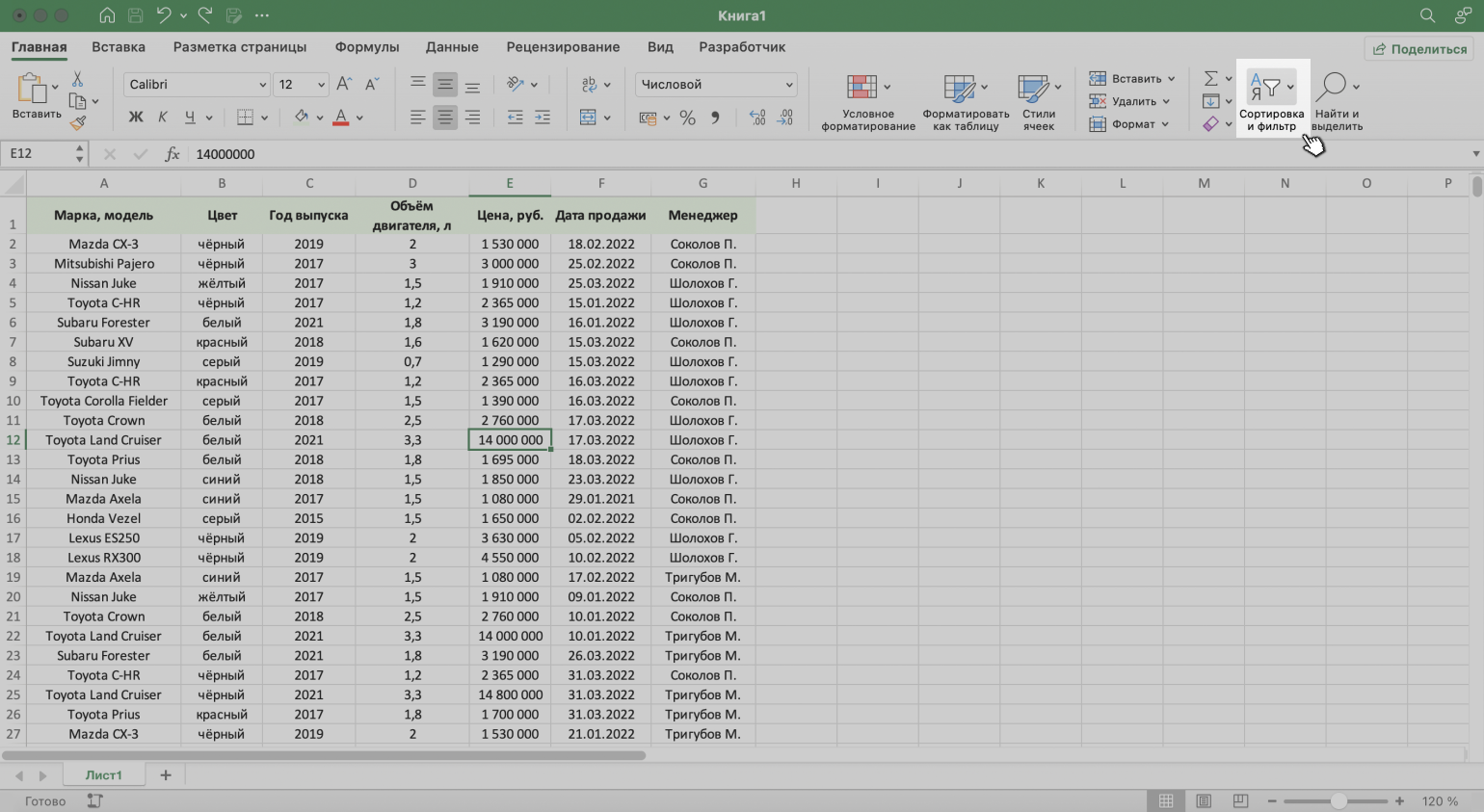
Для примера воспользуемся отчётностью небольшого автосалона. В таблице собрана информация о продажах: характеристики авто, цены, даты продажи и ответственные менеджеры.

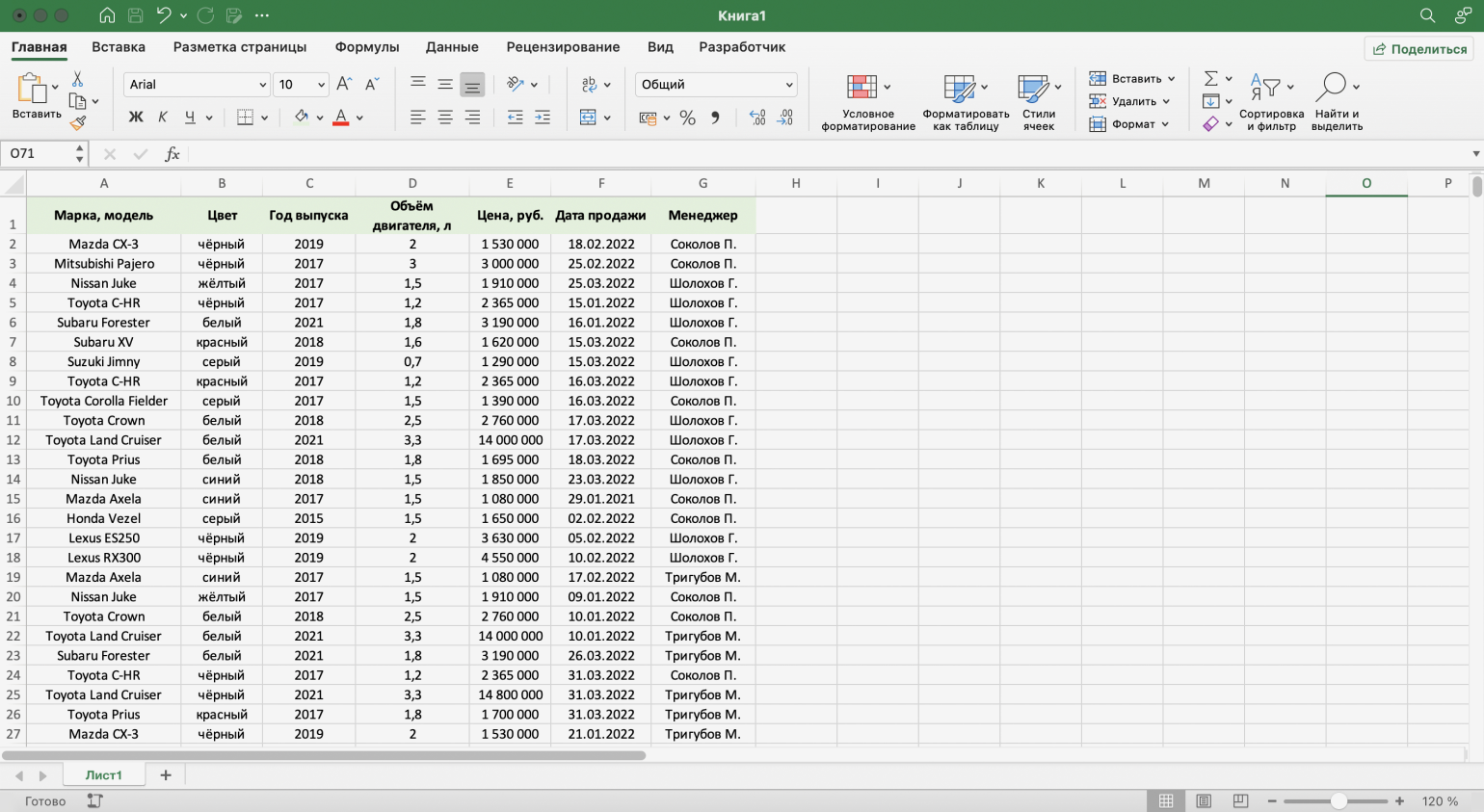
Таблица, в которой хранятся данные о продажах автосалона
Скриншот: Excel / Skillbox Media

Допустим, нужно показать продажи только одного менеджера — Соколова П. Воспользуемся фильтрацией.

Шаг 1. Выделяем ячейку внутри таблицы — не обязательно ячейку столбца «Менеджер», любую.

Чтобы настроить фильтрацию, выбираем любую ячейку таблицы
Скриншот: Excel / Skillbox Media

Шаг 2. На вкладке «Главная» нажимаем кнопку «Сортировка и фильтр».

Нажимаем кнопку «Сортировка и фильтр»
Скриншот: Excel / Skillbox Media

Шаг 3. В появившемся меню выбираем пункт «Фильтр».

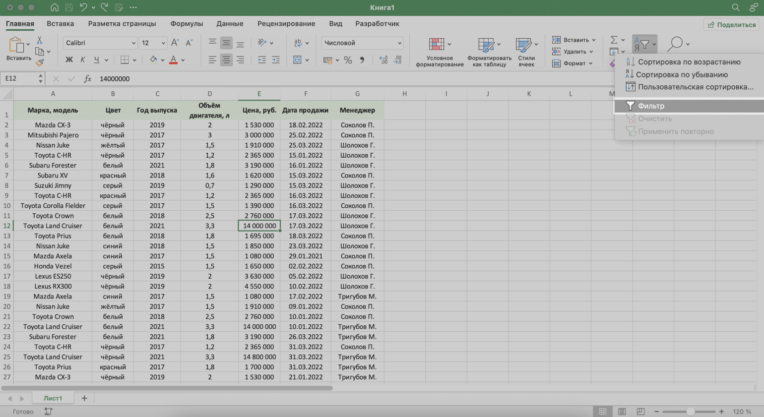
Жмём сюда, чтобы применить фильтрацию ко всем столбцам таблицы
Скриншот: Excel / Skillbox Media

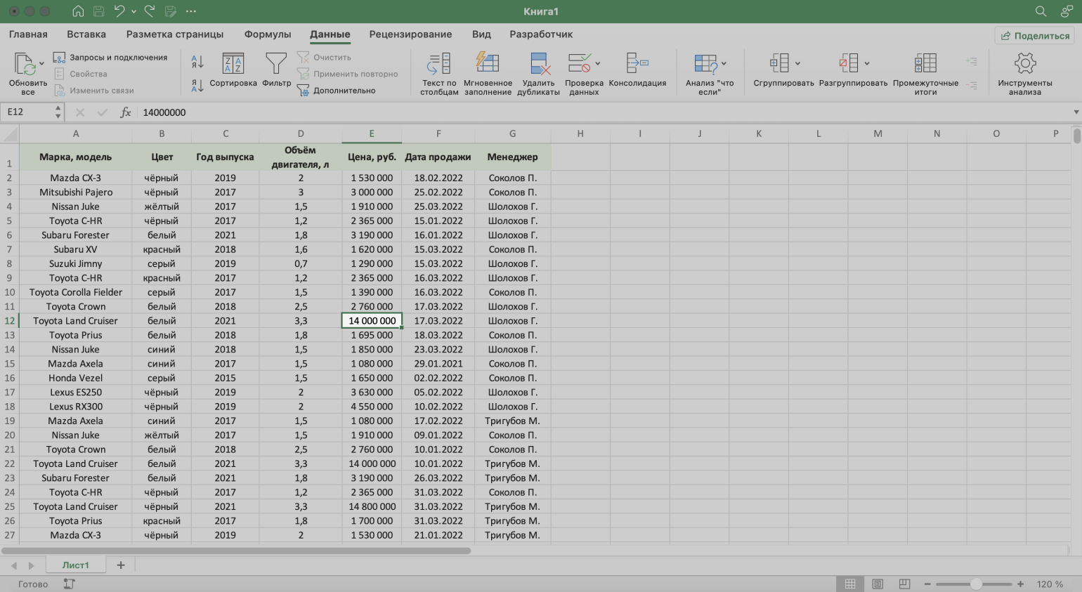
То же самое можно сделать через кнопку «Фильтр» на вкладке «Данные».

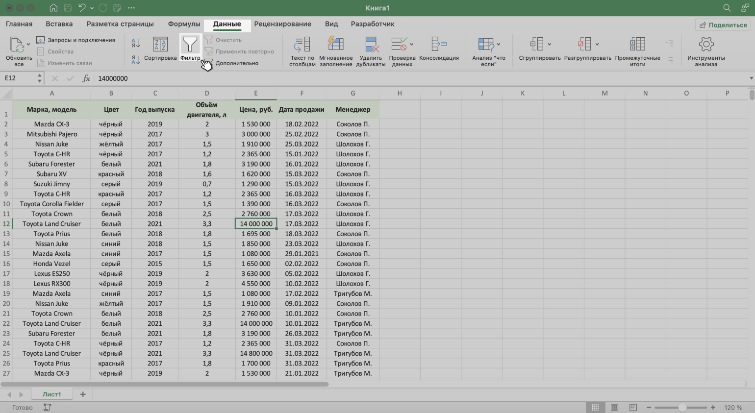
Второй способ установить фильтрацию
Скриншот: Excel / Skillbox Media

Шаг 4. В каждой ячейке шапки таблицы появились кнопки со стрелками — нажимаем на кнопку столбца, который нужно отфильтровать. В нашем случае это столбец «Менеджер».

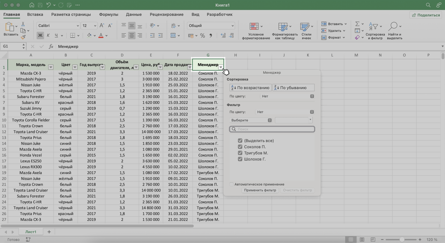
Нажимаем кнопку столбца, который нужно отфильтровать, — появляется меню фильтра
Скриншот: Excel / Skillbox Media

Шаг 5. В появившемся меню флажком выбираем данные, которые нужно оставить в таблице, — в нашем случае данные менеджера Соколова П., — и нажимаем кнопку «Применить фильтр».

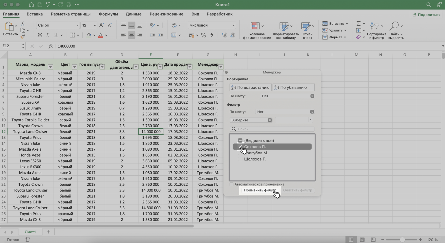
Выбираем менеджера, данные о продажах которого нужно показать в таблице
Скриншот: Excel / Skillbox Media

Готово — таблица показывает данные о продажах только одного менеджера. На кнопке со стрелкой появился дополнительный значок. Он означает, что в этом столбце настроена фильтрация.

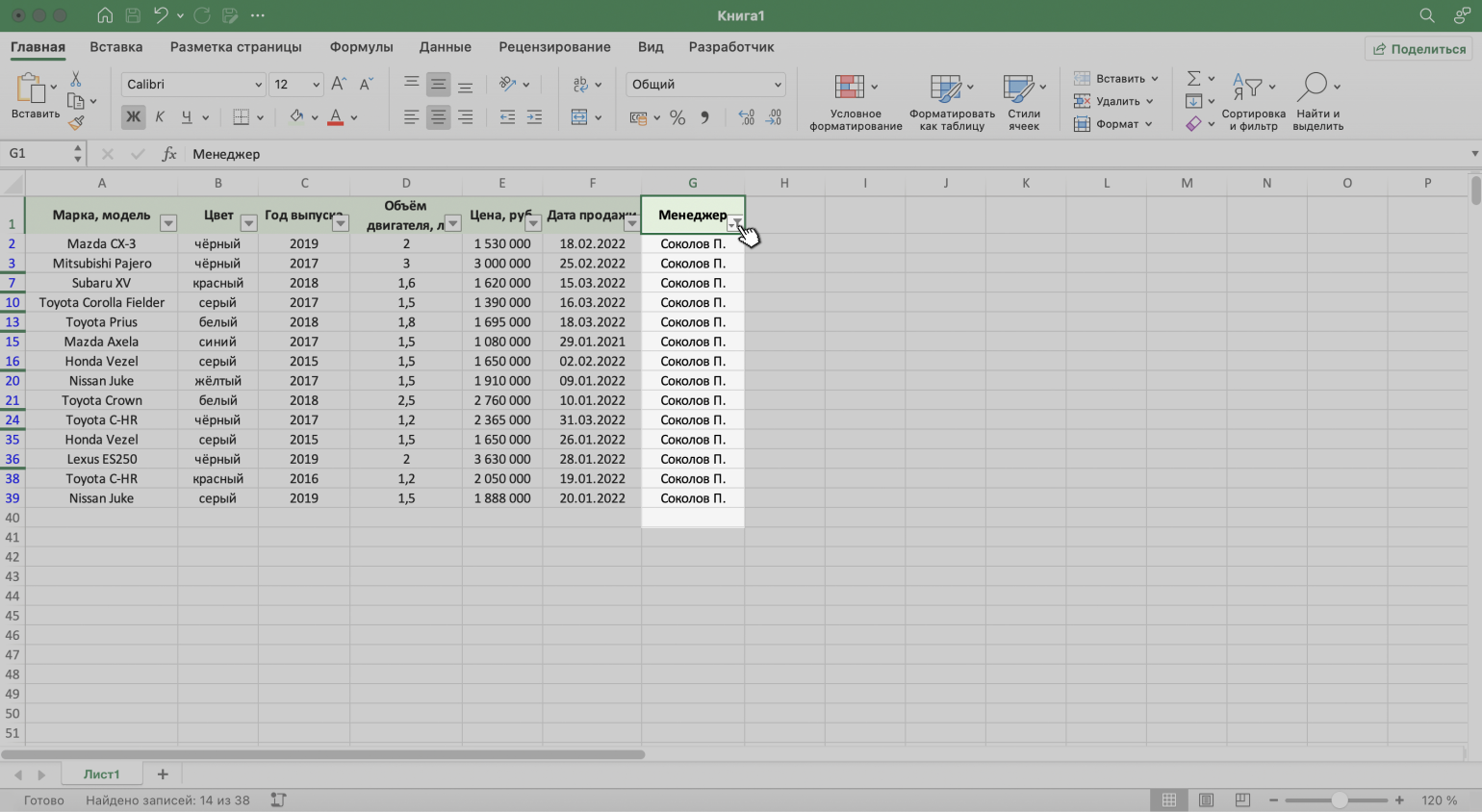
Результат фильтрации по одному параметру
Скриншот: Excel / Skillbox Media

Чтобы ещё уменьшить количество отображаемых в таблице данных, можно применять несколько фильтров одновременно. При этом как фильтр можно задавать не только точное значение ячеек, но и условие, которому отфильтрованные ячейки должны соответствовать.

Разберём на примере.

Выше мы уже отфильтровали таблицу по одному параметру — оставили в ней продажи только менеджера Соколова П. Добавим второй параметр — среди продаж Соколова П. покажем автомобили дороже 1,5 млн рублей.

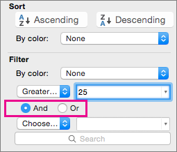
Шаг 1. Открываем меню фильтра для столбца «Цена, руб.» и нажимаем на параметр «Выберите».

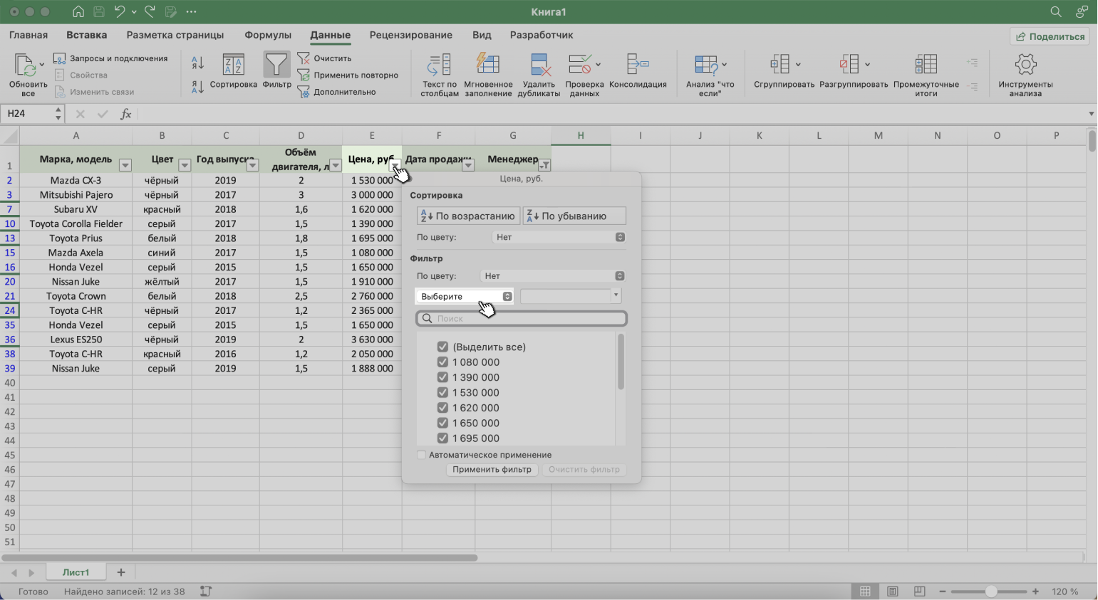
Открываем меню фильтра столбца «Цена, руб.» и жмём сюда
Скриншот: Excel / Skillbox Media

Шаг 2. Выбираем критерий, которому должны соответствовать отфильтрованные ячейки.

В нашем случае нужно показать автомобили дороже 1,5 млн рублей — выбираем критерий «Больше».

Выбираем критерий фильтрации
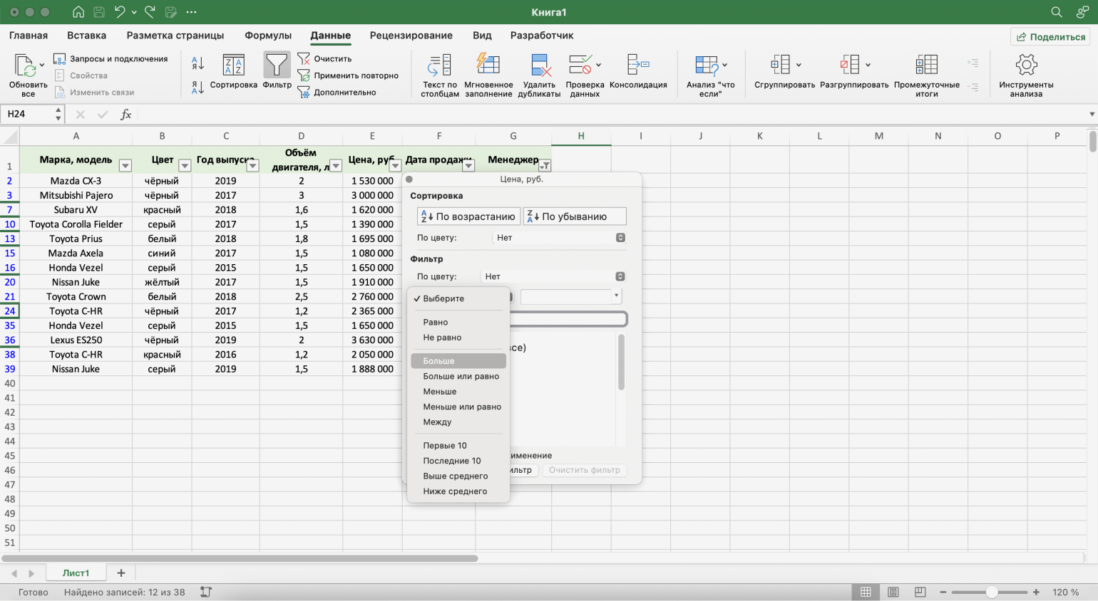
Скриншот: Excel / Skillbox Media

Шаг 3. Дополняем условие фильтрации — в нашем случае «Больше 1500000» — и нажимаем «Применить фильтр».

Дополняем условие фильтрации
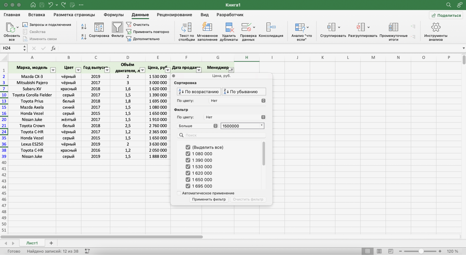
Скриншот: Excel / Skillbox Media

Готово — фильтрация сработала по двум параметрам. Теперь таблица показывает только те проданные менеджером авто, цена которых была выше 1,5 млн рублей.

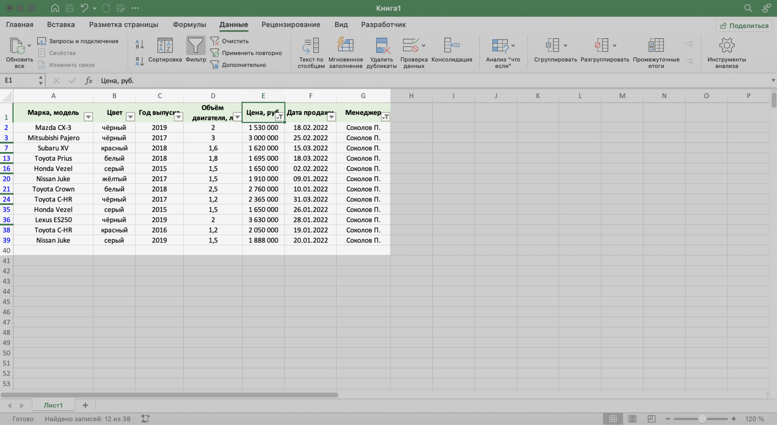
Результат фильтрации по двум параметрам
Скриншот: Excel / Skillbox Media

Расширенный фильтр позволяет фильтровать таблицу по сложным критериям сразу в нескольких столбцах.

Это можно сделать способом, который мы описали выше: поочерёдно установить несколько стандартных фильтров или фильтров с условиями пользователя. Но в случае с объёмными таблицами этот способ может быть неудобным и трудозатратным. Для экономии времени применяют расширенный фильтр.

Принцип работы расширенного фильтра следующий:

Копируют шапку исходной таблицы и создают отдельную таблицу для условий фильтрации.
Вводят условия.
Запускают фильтрацию.

Разберём на примере. Отфильтруем отчётность автосалона по трём критериям:

менеджер — Шолохов Г.;
год выпуска автомобиля — 2019-й или раньше;
цена — до 2 млн рублей.

Шаг 1. Создаём таблицу для условий фильтрации — для этого копируем шапку исходной таблицы и вставляем её выше.

Важное условие — между таблицей с условиями и исходной таблицей обязательно должна быть пустая строка.

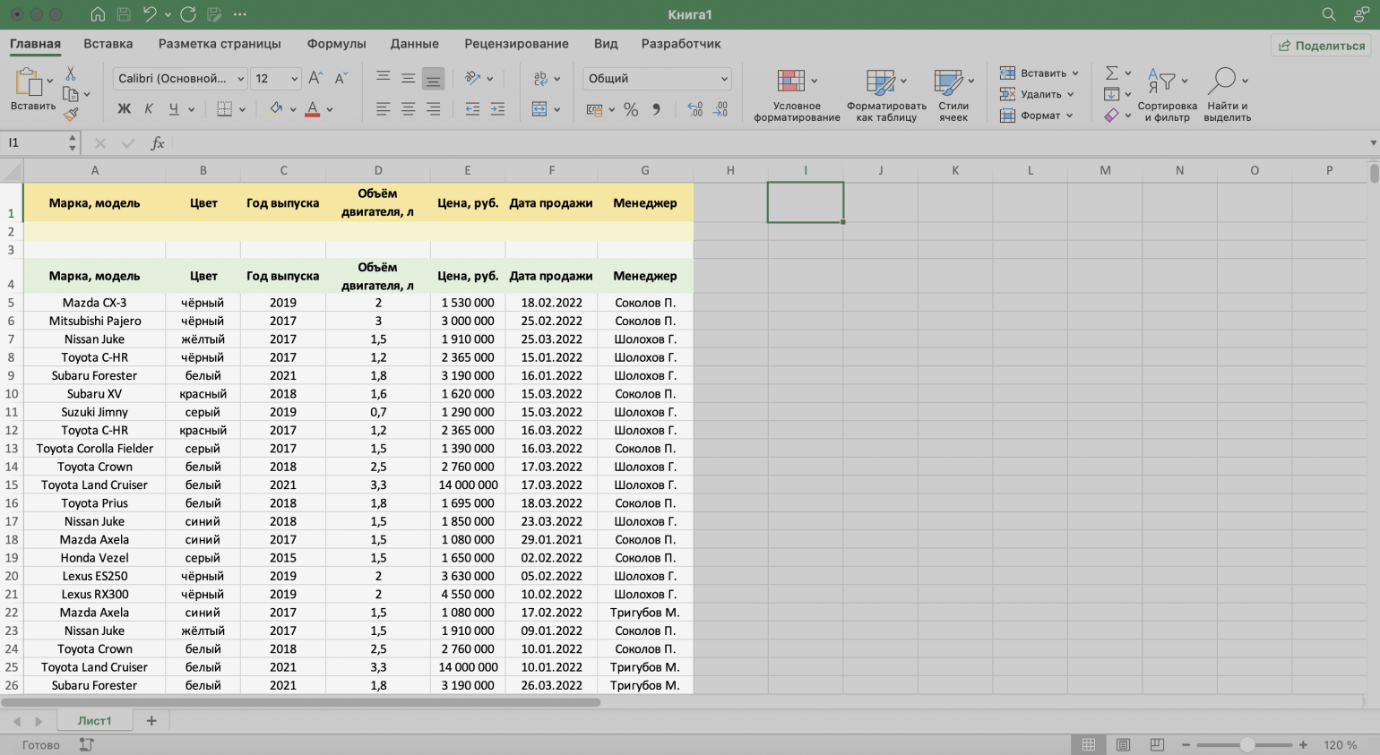
Создаём таблицу для условий фильтрации
Скриншот: Excel / Skillbox Media

Шаг 2. В созданной таблице вводим критерии фильтрации:

«Год выпуска» → <=2019.
«Цена, руб.» → <2000000.
«Менеджер» → Шолохов Г.

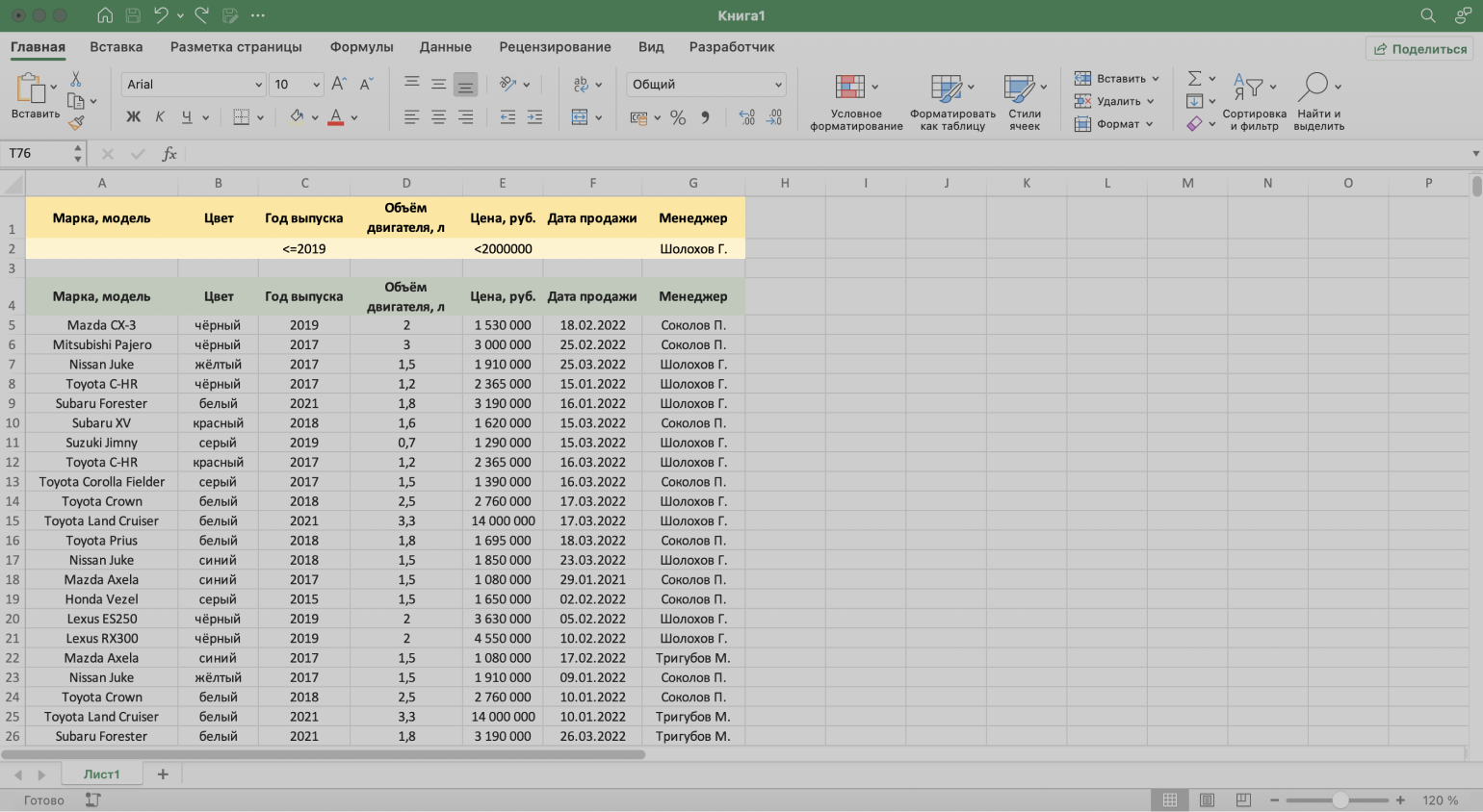
В таблице с условиями вводим критерии фильтрации
Скриншот: Excel / Skillbox Media

Шаг 3. Выделяем любую ячейку исходной таблицы и на вкладке «Данные» нажимаем кнопку «Дополнительно».

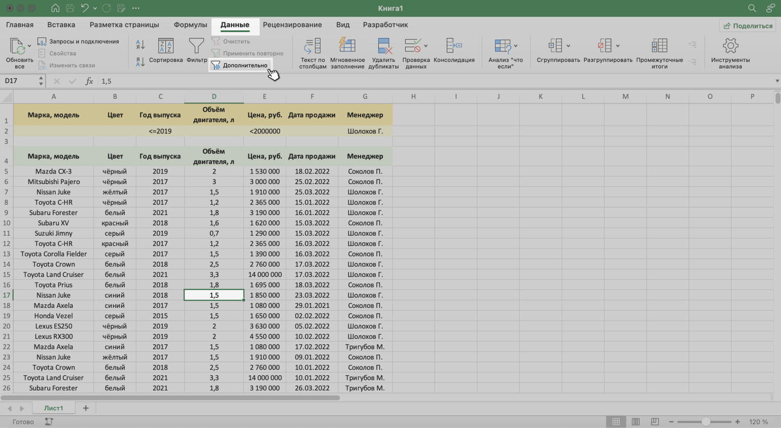
Выделяем ячейку исходной таблицы и нажимаем на «Дополнительно», чтобы вызвать меню расширенного фильтра
Скриншот: Excel / Skillbox Media

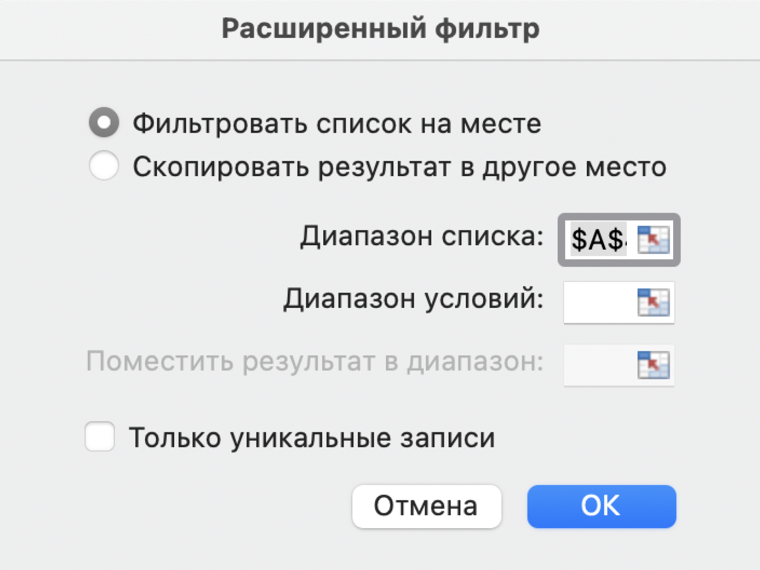
Шаг 4. В появившемся окне заполняем параметры расширенного фильтра:

Выбираем, где отобразятся результаты фильтрации: в исходной таблице или в другом месте. В нашем случае выберем первый вариант — «Фильтровать список на месте».
Диапазон списка — диапазон таблицы, для которой нужно применить фильтр. Он заполнен автоматически, для этого мы выделяли ячейку исходной таблицы перед тем, как вызвать меню.

Эти параметры меню выставлены программой автоматически
Скриншот: Excel / Skillbox Media

Диапазон условий — диапазон таблицы с условиями фильтрации. Ставим курсор в пустое окно параметра и выделяем диапазон: шапку таблицы и строку с критериями. Данные диапазона автоматически появляются в окне параметров расширенного фильтра.

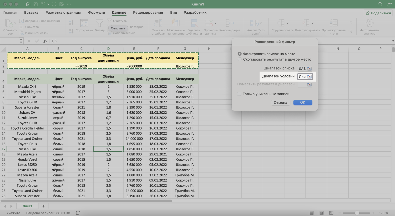
Выделяем диапазон таблицы с условиями
Скриншот: Excel / Skillbox Media

Шаг 5. Нажимаем «ОК» в меню расширенного фильтра.

Готово — исходная таблица отфильтрована по трём заданным параметрам.

Итог работы расширенного фильтра
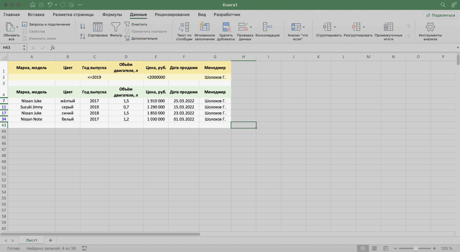
Скриншот: Excel / Skillbox Media

Отменить фильтрацию можно тремя способами:

1. Вызвать меню отфильтрованного столбца и нажать на кнопку «Очистить фильтр».

Первый способ снять фильтрацию
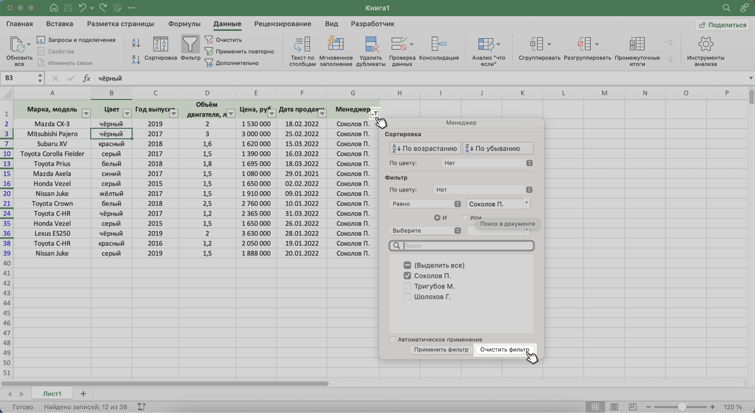
Скриншот: Excel / Skillbox Media

2. Нажать на кнопку «Сортировка и фильтр» на вкладке «Главная». Затем — либо снять галочку напротив пункта «Фильтр», либо нажать «Очистить фильтр».

Второй способ снять фильтрацию
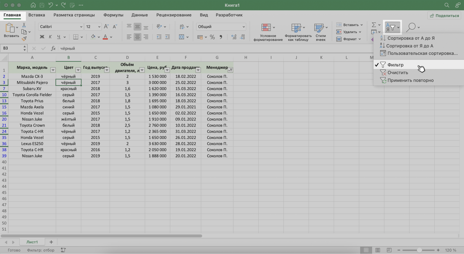
Скриншот: Excel / Skillbox Media

3. Нажать на кнопку «Очистить» на вкладке «Данные».

Третий способ снять фильтрацию
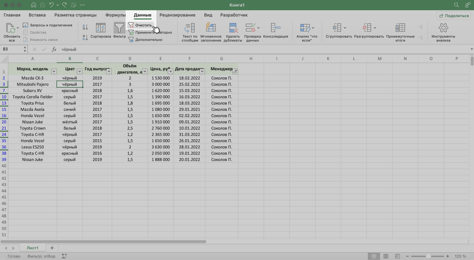
Скриншот: Excel / Skillbox Media

Научитесь: Excel + Google Таблицы с нуля до PRO
Узнать больше

Источник

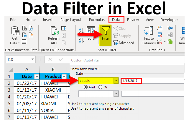
Data Filter in Excel (Table of Contents)

Data Filter in Excel
Uses of Data Filter in Excel
Types of Data Filter in Excel
How to Add Data Filter in Excel?

Data Filter in Excel

Data Filter in excel has many purposes apart from filtering the data. Although its main purpose is to filter the data as per the required condition, apart from this, we can sort, arrange the data, filter the data as per the color of cells or fonts or any condition available in the Text filter in the column where the filter is applied. To apply the filter, first, select the row where we need a filter, then from the Data menu tab, select Filter from Sort & Filter section. Or else we can apply filter by using short cut key ALT + D + F + F simultaneously or Ctrl + Shift + L together.

Uses of Data Filter in Excel

If the table or range contains a huge number of datasets, it’s very difficult to find & extract the precise requested information or data. In this scenario, the Data Filter helps out.

Filter

Data Filter in Excel option helps out in many ways to filter the data based on text, value, numeric or date value.
The Data Filter option is very helpful to sort out data with simple drop-down menus.
The Data Filter option is significant to temporarily hide few data sets in a table so that you can focus on the relevant data we need to work on.
Filters are applied to rows of data in the worksheet.
Apart from multiple filtering options, auto-filter criteria provide the Sort options also relevant to a given column.

Definition

Data Filter in Excel: it’s a quick way to display only the relevant or specific information which we need & temporarily hide irrelevant information or data in a table.

To activate the Excel data filter for any data in excel, select the entire data range or table range and click on the Filter button in the Data tab in the Excel ribbon.

(keyboard shortcut – Control + Shift + L)

Types of Data Filter in Excel

There are three types of data filtering options:

1. Data Filter Based On Text Values – It is used when the cells contain TEXT values; it has below mentioned Filtering Operators (Explained in example 1).

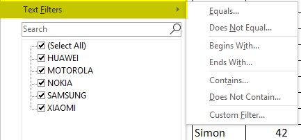
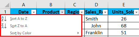
Apart from multiple filtering options in a text value, AutoFilter criteria provide the Sort options also relevant to a given column. i.e. Sort by A to Z, Sort by Z to A, and Sort by Color.

2. Data Filter Based on Numeric Values – It is used when the cells contain numbers or numeric values

It has below mentioned Filtering Operators (Explained in example 2)

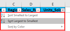
Apart from multiple filtering options in Numeric value, AutoFilter criteria provide the Sort options also relevant to a given column. i.e. Sort by Smallest to Largest, Sort by Largest to Smallest, and Sort by Color.

3. Data Filter Based On Date Values – It is used when the cells contain date values (Explained in example 3)

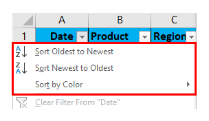
Apart from multiple filtering options in date value, AutoFilter criteria provide the Sort options also relevant to a given column. i.e. Sort by Oldest to Newest, Sort by Newest to Oldest, and Sort by Color.

How to Add Data Filter in Excel?

This Data Filter is very simple easy to use. Let us now see how to Add a Data Filter in Excel with the help of some examples.

You can download this Data Filter Excel Template here – Data Filter Excel Template

Example #1 – Filtering Based on Text Values or Data

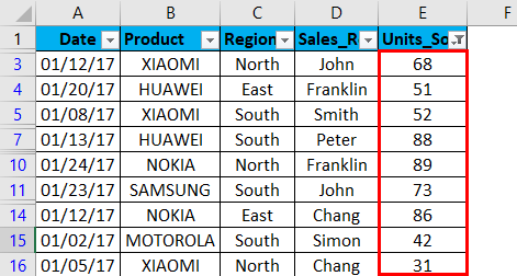
In the below-mentioned example, the Mobile sales data table contains a huge list of datasets.

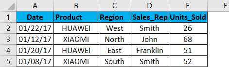
Initially, I have to activate the Excel data filter for the Mobile sales data table in excel, select the entire data range or table range, and click on the Filter button in the Data tab in the Excel ribbon.

Or click (keyboard shortcut – Control + Shift + L)

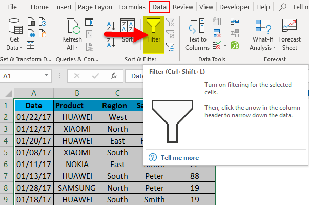
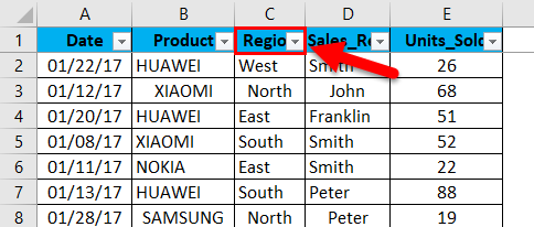
When you click on Filter, each column in the first row will automatically have a small drop-down button or filter icon added at the right corner of the cell i.e.

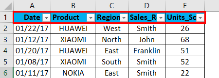
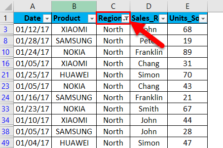
When excel identifies that the column contains text data, it automatically displays the option of text filters. In the mobile sales data, if I want sales data in the northern region only, irrespective of date, product, sales rep & units sold. I need to select the filter icon in the region header; I have to uncheck or deselect all the regions except the north region. It returns mobile sales data in the northern region only.

Once a filter is applied in the region column, Excel pinpoints you that table is filtered on a particular column by adding a funnel icon to the region column’s drop-down list button.

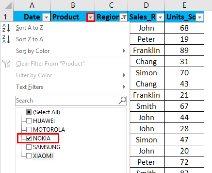
I can further filter based on brand & sales rep data. Now with this data, I further filter in the product region where I want the sales of the Nokia brand in the north region only irrespective of the sales rep, units sold & date.

I have to just apply the filter in the product column apart from the region column. I have to uncheck or deselect all the products except the NOKIA brand. It returns Nokia sales data in the north region.

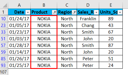
Once the filter is applied in the product column, Excel pinpoints you that table is filtered on a particular column by adding a funnel icon to the product column’s drop-down list button.

Example #2 – Filtering Based on Numeric Values or Data

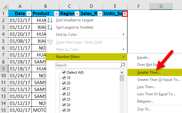
When excel identifies that the column contains NUMERIC values or data, it automatically displays the option of text filters.

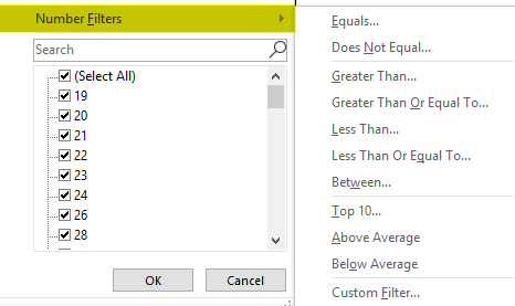
If I want data of units sold in the mobile sales data, which is more than 30 units, irrespective of date, product, sales rep & region. For that, I need to select the filter icon in the units sold header; I have to select the number of filters, and under that greater than an option.

Once greater than option under number filter is selected, pop up appears, i.e. Custom auto filter, in that under the unit sold, we want datasets of more than 30 units sold, so enter 30. Click ok.

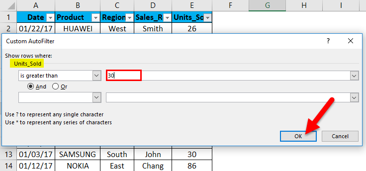
It returns mobile sales data based on the units sold. i.e. more than 30 units only.

Once the filter is applied in the units sold column, Excel pinpoints you that table is filtered on a particular column by adding a funnel icon to the units sold column drop-down list button.

Sales data can be further Sorted by Smallest to Largest or Largest to Smallest in units sold.

Example #3 – Filtering based on Date Value

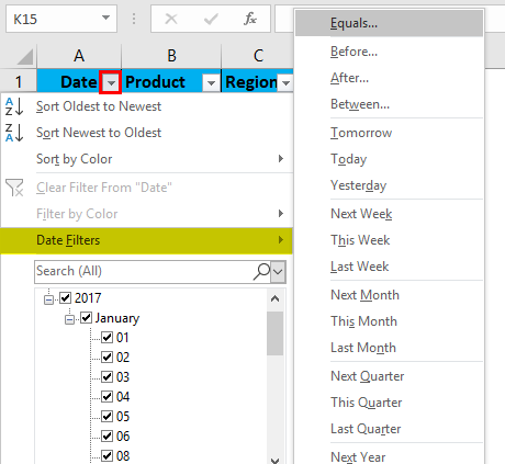
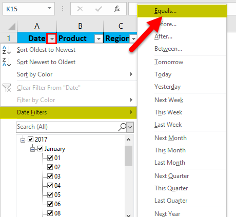
When excel identifies that the column contains DATE values or data, it automatically displays the option of DATE filters.

Date filter lets you filter dates based on any date range. For example, you can filter on conditions such dates by day, week, month, year, quarter, or year-to-date.

In the mobile sales data, if I want mobile sales data only on or for the date value, i.e. 01/15/17, irrespective of units sold, product, sales rep & region. I need to select the filter icon in the date header; I have to select the date filter, and under that equals to option.

Custom AutoFilter dialog box will appear; enter a date value manually, i.e. 01/15/17

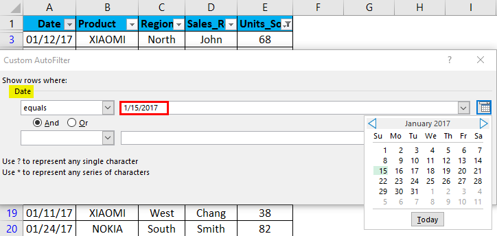
Click ok. It returns mobile sales data only on or for the date value, i.e. 01/15/17

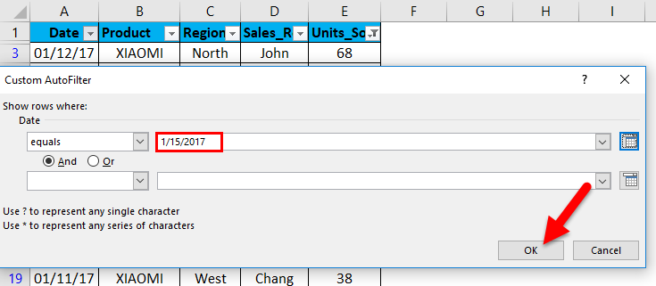
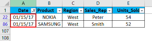
Once a filter is applied in the date column, Excel pinpoints you that table is filtered on a particular column by adding a funnel icon to the date column drop-down list button.

Things to Remember

Data filter helps out to specify the required data that you want to display. This process is also called “Grouping of data, ” which helps out better analyse your data.
Excel data can also be used to search or filter a data set with a specific word in a text with the help of a custom auto filter on the condition it contains ‘a’ or any relevant word of your choice.
Data Filter option can be removed with the below-mentioned steps:

Go to the Data tab > Sort & Filter group and click Clear.

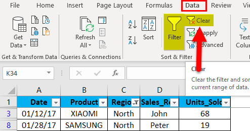
A Data Filter option is Removed.

Excel data filter option can filter the records by multiple criteria or conditions, i.e. by filtering multiple column values (more than one column) explained in example 1.
Excel data filter helps out to sort out blank & non-blank cells in the column.
Data can also be filtered out with the help of wild characters, i.e.? (question mark) & * (asterisk) & ~ (tilde)

Try it!

Filter a range of data

Filter data in a table

Want more?

Need more help?

Want more options?

Filter a range of data

Filter data in a table

Related Topics

Filter data in a table

Filter a range of data

Filtering options for tables or ranges

To clear a filter from a column

To remove all the filters from a table or range

Need more help?

Basic example

Filter for Red group

No matching data

Values that contain text

Filter by date

Multiple criteria

Complex criteria

Notes

Data Filter in Excel

Uses of Data Filter in Excel

Types of Data Filter in Excel

How to Add Data Filter in Excel?

Example #1 – Filtering Based on Text Values or Data

Example #2 – Filtering Based on Numeric Values or Data

Example #3 – Filtering based on Date Value

Things to Remember

Recommended Articles