

A lot of Excel functionalities are also available to be used in VBA – and the Autofilter method is one such functionality.
If you have a dataset and you want to filter it using a criterion, you can easily do it using the Filter option in the Data ribbon.![]()
And if you want a more advanced version of it, there is an advanced filter in Excel as well.
Then Why Even Use the AutoFilter in VBA?
If you just need to filter data and do some basic stuff, I would recommend stick to the inbuilt Filter functionality that Excel interface offers.
You should use VBA Autofilter when you want to filter the data as a part of your automation (or if it helps you save time by making it faster to filter the data).
For example, suppose you want to quickly filter the data based on a drop-down selection, and then copy this filtered data into a new worksheet.
While this can be done using the inbuilt filter functionality along with some copy-paste, it can take you a lot of time to do this manually.
In such a scenario, using VBA Autofilter can speed things up and save time.
Note: I will cover this example (on filtering data based on a drop-down selection and copying into a new sheet) later in this tutorial.
Excel VBA Autofilter Syntax
Expression. AutoFilter( _Field_ , _Criteria1_ , _Operator_ , _Criteria2_ , _VisibleDropDown_ )
- Expression: This is the range on which you want to apply the auto filter.
- Field: [Optional argument] This is the column number that you want to filter. This is counted from the left in the dataset. So if you want to filter data based on the second column, this value would be 2.
- Criteria1: [Optional argument] This is the criteria based on which you want to filter the dataset.
- Operator: [Optional argument] In case you’re using criteria 2 as well, you can combine these two criteria based on the Operator. The following operators are available for use: xlAnd, xlOr, xlBottom10Items, xlTop10Items, xlBottom10Percent, xlTop10Percent, xlFilterCellColor, xlFilterDynamic, xlFilterFontColor, xlFilterIcon, xlFilterValues
- Criteria2: [Optional argument] This is the second criteria on which you can filter the dataset.
- VisibleDropDown: [Optional argument] You can specify whether you want the filter drop-down icon to appear in the filtered columns or not. This argument can be TRUE or FALSE.
Apart from Expression, all the other arguments are optional.
In case you don’t use any argument, it would simply apply or remove the filter icons to the columns.
Sub FilterRows()
Worksheets("Filter Data").Range("A1").AutoFilter
End Sub
The above code would simply apply the Autofilter method to the columns (or if it’s already applied, it will remove it).
This simply means that if you can not see the filter icons in the column headers, you will start seeing it when this above code is executed, and if you can see it, then it will be removed.
In case you have any filtered data, it will remove the filters and show you the full dataset.
Now let’s see some examples of using Excel VBA Autofilter that will make it’s usage clear.
Example: Filtering Data based on a Text condition
Suppose you have a dataset as shown below and you want to filter it based on the ‘Item’ column.
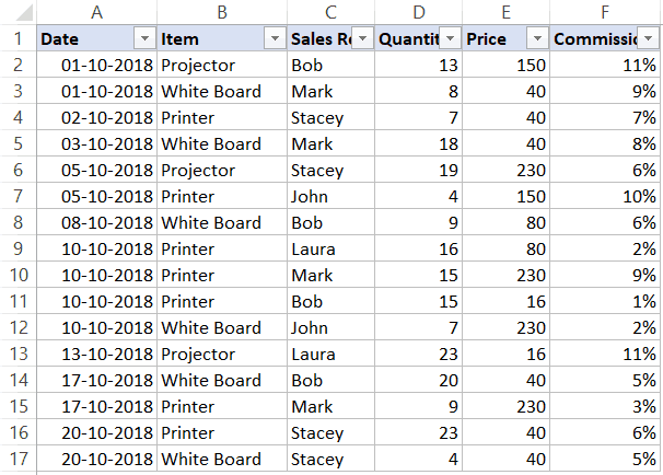
The below code would filter all the rows where the item is ‘Printer’.
Sub FilterRows()
Worksheets("Sheet1").Range("A1").AutoFilter Field:=2, Criteria1:="Printer"
End Sub
The above code refers to Sheet1 and within it, it refers to A1 (which is a cell in the dataset).
Note that here we have used Field:=2, as the item column is the second column in our dataset from the left.
Now if you’re thinking – why do I need to do this using a VBA code. This can easily be done using inbuilt filter functionality.
You’re right!
If this is all you want to do, better used the inbuilt Filter functionality.
But as you read the remaining tutorial, you’ll see that this can be combined with some extra code to create powerful automation.
But before I show you those, let me first cover a few examples to show you what all the AutoFilter method can do.
Click here to download the example file and follow along.
Example: Multiple Criteria (AND/OR) in the Same Column
Suppose I have the same dataset, and this time I want to filter all the records where the item is either ‘Printer’ or ‘Projector’.
The below code would do this:
Sub FilterRowsOR()
Worksheets("Sheet1").Range("A1").AutoFilter Field:=2, Criteria1:="Printer", Operator:=xlOr, Criteria2:="Projector"
End Sub
Note that here I have used the xlOR operator.
This tells VBA to use both the criteria and filter the data if any of the two criteria are met.
Similarly, you can also use the AND criteria.
For example, if you want to filter all the records where the quantity is more than 10 but less than 20, you can use the below code:
Sub FilterRowsAND()
Worksheets("Sheet1").Range("A1").AutoFilter Field:=4, Criteria1:=">10", _
    Operator:=xlAnd, Criteria2:="<20"
End Sub
Example: Multiple Criteria With Different Columns
Suppose you have the following dataset.
With Autofilter, you can filter multiple columns at the same time.
For example, if you want to filter all the records where the item is ‘Printer’ and the Sales Rep is ‘Mark’, you can use the below code:
Sub FilterRows()
With Worksheets("Sheet1").Range("A1")
.AutoFilter field:=2, Criteria1:="Printer"
.AutoFilter field:=3, Criteria1:="Mark"
End With
End Sub
Example: Filter Top 10 Records Using the AutoFilter Method
Suppose you have the below dataset.
Below is the code that will give you the top 10 records (based on the quantity column):
Sub FilterRowsTop10()
ActiveSheet.Range("A1").AutoFilter Field:=4, Criteria1:="10", Operator:=xlTop10Items
End Sub
In the above code, I have used ActiveSheet. You can use the sheet name if you want.
Note that in this example, if you want to get the top 5 items, just change the number in Criteria1:=”10″ from 10 to 5.
So for top 5 items, the code would be:
Sub FilterRowsTop5()
ActiveSheet.Range("A1").AutoFilter Field:=4, Criteria1:="5", Operator:=xlTop10Items
End Sub
It may look weird, but no matter how many top items you want, the Operator value always remains xlTop10Items.
Similarly, the below code would give you the bottom 10 items:
Sub FilterRowsBottom10()
ActiveSheet.Range("A1").AutoFilter Field:=4, Criteria1:="10", Operator:=xlBottom10Items
End Sub
And if you want the bottom 5 items, change the number in Criteria1:=”10″ from 10 to 5.
Example: Filter Top 10 Percent Using the AutoFilter Method
Suppose you have the same data set (as used in the previous examples).
Below is the code that will give you the top 10 percent records (based on the quantity column):
Sub FilterRowsTop10()
ActiveSheet.Range("A1").AutoFilter Field:=4, Criteria1:="10", Operator:=xlTop10Percent
End Sub
In our dataset, since we have 20 records, it will return the top 2 records (which is 10% of the total records).
Example: Using Wildcard Characters in Autofilter
Suppose you have a dataset as shown below:
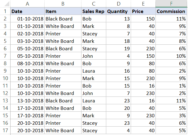
If you want to filter all the rows where the item name contains the word ‘Board’, you can use the below code:
Sub FilterRowsWildcard()
Worksheets("Sheet1").Range("A1").AutoFilter Field:=2, Criteria1:="*Board*"
End Sub
In the above code, I have used the wildcard character * (asterisk) before and after the word ‘Board’ (which is the criteria).
An asterisk can represent any number of characters. So this would filter any item that has the word ‘board’ in it.
Example: Copy Filtered Rows into a New Sheet
If you want to not only filter the records based on criteria but also copy the filtered rows, you can use the below macro.
It copies the filtered rows, adds a new worksheet, and then pastes these copied rows into the new sheet.
Sub CopyFilteredRows()
Dim rng As Range
Dim ws As Worksheet
If Worksheets("Sheet1").AutoFilterMode = False Then
MsgBox "There are no filtered rows"
Exit Sub
End If
Set rng = Worksheets("Sheet1").AutoFilter.Range
Set ws = Worksheets.Add
rng.Copy Range("A1")
End Sub
The above code would check if there are any filtered rows in Sheet1 or not.
If there are no filtered rows, it will show a message box stating that.
And if there are filtered rows, it will copy those, insert a new worksheet, and paste these rows on that newly inserted worksheet.
Example: Filter Data based on a Cell Value
Using Autofilter in VBA along with a drop-down list, you can create a functionality where as soon as you select an item from the drop-down, all the records for that item are filtered.
Something as shown below:
 Click here to download the example file and follow along.
This type of construct can be useful when you want to quickly filter data and then use it further in your work.
Below is the code that will do this:
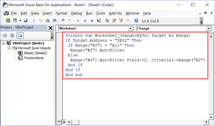
Private Sub Worksheet_Change(ByVal Target As Range)
If Target.Address = "$B$2" Then
 If Range("B2") = "All" Then
  Range("A5").AutoFilter
 Else
  Range("A5").AutoFilter Field:=2, Criteria1:=Range("B2")
 End If
End If
End Sub
This is a worksheet event code, which gets executed only when there is a change in the worksheet and the target cell is B2 (where we have the drop-down).
Also, an If Then Else condition is used to check if the user has selected ‘All’ from the drop down. If All is selected, the entire data set is shown.
This code is NOT placed in a module.
Instead, it needs to be placed in the backend of the worksheet that has this data.
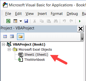
Here are the steps to put this code in the worksheet code window:
- Open the VB Editor (keyboard shortcut – ALT + F11).
- In the Project Explorer pane, double-click on the Worksheet name in which you want this filtering functionality.

- In the worksheet code window, copy and paste the above code.

- Close the VB Editor.
Now when you use the drop-down list, it will automatically filter the data.
This is a worksheet event code, which gets executed only when there is a change in the worksheet and the target cell is B2 (where we have the drop-down).
Also, an If Then Else condition is used to check if the user has selected ‘All’ from the drop down. If All is selected, the entire data set is shown.
Turn Excel AutoFilter ON/OFF using VBA
When applying Autofilter to a range of cells, there may already be some filters in place.
You can use the below code turn off any pre-applied auto filters:
Sub TurnOFFAutoFilter()
  Worksheets("Sheet1").AutoFilterMode = False
End Sub
This code checks the entire sheets and removes any filters that have been applied.
If you don’t want to turn off filters from the entire sheet but only from a specific dataset, use the below code:
Sub TurnOFFAutoFilter()
  If Worksheets("Sheet1").Range("A1").AutoFilter Then
    Worksheets("Sheet1").Range("A1").AutoFilter
  End If
End Sub
The above code checks whether there are already filters in place or not.
If filters are already applied, it removes it, else it does nothing.
Similarly, if you want to turn on AutoFilter, use the below code:
Sub TurnOnAutoFilter()
  If Not Worksheets("Sheet1").Range("A4").AutoFilter Then
    Worksheets("Sheet1").Range("A4").AutoFilter
  End If
End Sub
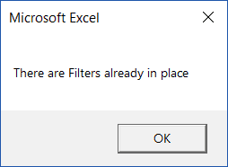
Check if AutoFilter is Already Applied
If you have a sheet with multiple datasets and you want to make sure you know that there are no filters already in place, you can use the below code.
Sub CheckforFilters()
If ActiveSheet.AutoFilterMode = True Then
MsgBox "There are Filters already in place"
Else
MsgBox "There are no filters"
End If
End Sub
This code uses a message box function that displays a message ‘There are Filters already in place’ when it finds filters on the sheet, else it shows ‘There are no filters’.
Show All Data
If you have filters applied to the dataset and you want to show all the data, use the below code:
Sub ShowAllData()
If ActiveSheet.FilterMode Then ActiveSheet.ShowAllData
End Sub
The above code checks whether the FilterMode is TRUE or FALSE.
If it’s true, it means a filter has been applied and it uses the ShowAllData method to show all the data.
Note that this does not remove the filters. The filter icons are still available to be used.
Using AutoFilter on Protected Sheets
By default, when you protect a sheet, the filters won’t work.
In case you already have filters in place, you can enable AutoFilter to make sure it works even on protected sheets.
To do this, check the Use Autofilter option while protecting the sheet.
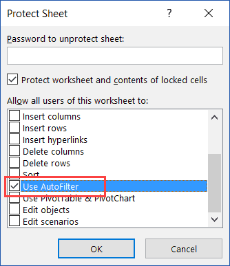
While this works when you already have filters in place, in case you try to add Autofilters using a VBA code, it won’t work.
Since the sheet is protected, it wouldn’t allow any macro to run and make changes to the Autofilter.
So you need to use a code to protect the worksheet and make sure auto filters are enabled in it.
This can be useful when you have created a dynamic filter (something I covered in the example – ‘Filter Data based on a Cell Value’).
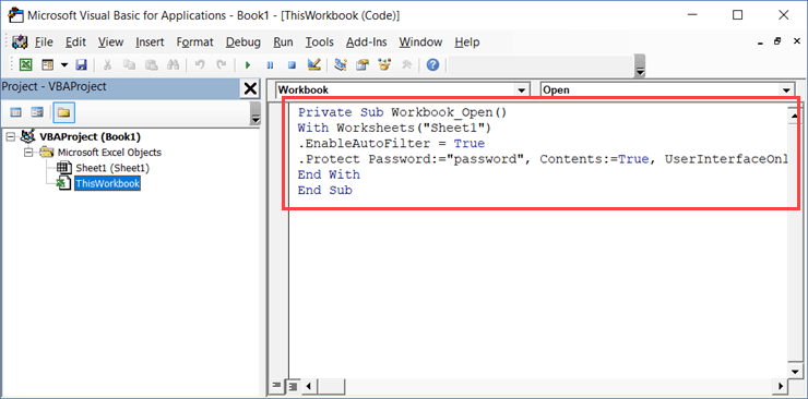
Below is the code that will protect the sheet, but at the same time, allow you to use Filters as well as VBA macros in it.
Private Sub Workbook_Open()
With Worksheets("Sheet1")
.EnableAutoFilter = True
.Protect Password:="password", Contents:=True, UserInterfaceOnly:=True
End With
End Sub
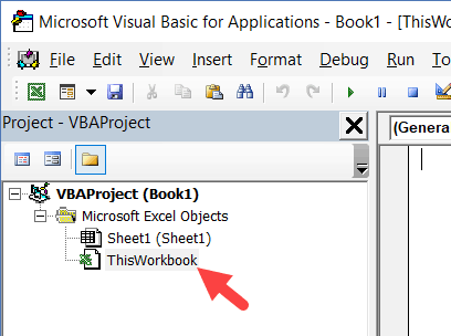
This code needs to be placed in ThisWorkbook code window.
Here are the steps to put the code in ThisWorkbook code window:
- Open the VB Editor (keyboard shortcut – ALT + F11).
- In the Project Explorer pane, double-click on the ThisWorkbook object.

- In the code window that opens, copy and paste the above code.

As soon as you open the workbook and enable macros, it will run the macro automatically and protect Sheet1.
However, before doing that, it will specify ‘EnableAutoFilter = True’, which means that the filters would work in the protected sheet as well.
Also, it sets the ‘UserInterfaceOnly’ argument to ‘True’. This means that while the worksheet is protected, the VBA macros code would continue to work.
You May Also Like the Following VBA Tutorials:
- Excel VBA Loops.
- Filter Cells with Bold Font Formatting.
- Recording a Macro.
- Sort Data Using VBA.
- Sort Worksheet Tabs in Excel.
 In this Excel VBA Tutorial, you learn to filter data in Excel with macros.
This Excel VBA AutoFilter Tutorial is accompanied by an Excel workbook containing the data and macros I use in the examples below. You can get free access to this example workbook by clicking the button below.

Use the following Table of Contents to navigate to the Section you’re interested in.
Related Excel VBA and Macro Training Materials
The following VBA and Macro training materials may help you better understand and implement the contents below:
- Tutorials about general VBA constructs and structures:
- Tutorials for Beginners:
- Macro Tutorial for Beginners.
- VBA Tutorial for Beginners.
- Enable macros in Excel.
- Work with the Visual Basic Editor (VBE).
- Create Sub procedures.
- Refer to objects, including:
- Sheets.
- Cells.
- Work with properties and methods.
- Declare variables and data types.
- Create R1C1-style references.
- Use Excel worksheet functions in VBA.
- Work with arrays.
- Tutorials for Beginners:
- Tutorials with practical VBA applications and macro examples:
- Find last row.
- Set or get a cell’s value.
- Copy paste.
- Search and find.
- Create message boxes.
- The comprehensive and actionable Books at The Power Spreadsheets Library:
- Excel Macros for Beginners Book Series.
- VBA Fundamentals Book Series.
#1. Excel VBA AutoFilter Column Based on Cell Value
VBA Code to AutoFilter Column Based on Cell Value
To AutoFilter a column based on a cell value, use the following structure/template in the applicable statement:
RangeObjectColumnToFilter.AutoFilter Field:=1, Criteria1:="ComparisonOperator" & RangeObjectCriteria.Value
The following Sections describe the main elements in this structure.
RangeObjectColumnToFilter
A Range object representing the column you AutoFilter.
AutoFilter
The Range.AutoFilter method filters a list with Excel’s AutoFilter.
Field:=1
The Field parameter of the Range.AutoFilter method:
- Specifies the field offset (column number) on which you base the AutoFilter.
- Is specified as an integer, with the first/leftmost column in the AutoFiltered cell range (RangeObjectColumnToFilter) being field 1.
To AutoFilter a column based on a cell value, set the Field parameter to 1.
Criteria1:=”ComparisonOperator” & RangeObjectCriteria.Value
The Criteria1 parameter of the Range.AutoFilter method is:
- As a general rule, a string specifying the AutoFiltering criteria.
- Subject to a variety of rules. The specific rules (usually) depend on the data type of the AutoFiltered column.
To AutoFilter a column based on a cell value (and as a general rule), set the Criteria1 parameter to a string specifying the AutoFiltering criteria by specifying:
- A comparison operator (ComparisonOperator); and
- The cell (RangeObjectCriteria) whose value you use to AutoFilter the column.
For these purposes:
- “ComparisonOperator” is a comparison operator specifying the type of comparison VBA carries out.
- “&” is the concatenation operator.
- “RangeObjectCriteria” is a Range object representing the cell whose value you use to AutoFilter the column (RangeObjectColumnToFilter).
- “Value” refers to the Range.Value property. The Range.Value property returns the value/string stored in the applicable cell (RangeObjectCriteria).
Macro Example to AutoFilter Column Based on Cell Value
The macro below does the following:
- Filter column A (with the data set starting in cell A6) of the worksheet named “AutoFilter Column Cell Value” in the workbook where the procedure is stored.
- Display (only) entries whose value is not equal to the value stored in cell D6 of the worksheet named “AutoFilter Column Cell Value” in the workbook where the procedure is stored.
Sub AutoFilterColumnCellValue()
    'Source: https://powerspreadsheets.com/
    'For further information: https://powerspreadsheets.com/excel-vba-autofilter/

    'This procedure:
        '(1) Filters the column/data starting on cell A6 of the "AutoFilter Column Cell Value" worksheet in this workbook based on the value stored in cell D6 of the same worksheet
        '(2) Displays (only) entries whose value is not equal to (<>) the value stored in cell D6 of the "AutoFilter Column Cell Value" worksheet in this workbook

    With ThisWorkbook.Worksheets("AutoFilter Column Cell Value")
        .Range("A6").AutoFilter Field:=1, Criteria1:="<>" & .Range("D6").Value
    End With

End Sub
Effects of Executing Macro Example to AutoFilter Column Based on Cell Value
The image below illustrates the effects of using the macro example. In this example:
- Column A (cells A6 to A31) contains:
- A header (cell A6); and
- Randomly generated values (cells A7 to A31).
- Cell D6 contains a randomly generated value (8).
- A text box (Filter column A based on value of cell D6) executes the macro example when clicked.
When the macro is executed, Excel:
- Filters column A based on the value in cell D6.
- Displays (only) entries whose value is not equal to the value in cell D6 (8).

#2. Excel VBA AutoFilter Table Based on 1 Column and 1 Cell Value
VBA Code to AutoFilter Table Based on 1 Column and 1 Cell Value
To AutoFilter a table based on 1 column and 1 cell value, use the following structure/template in the applicable statement:
RangeObjectTableToFilter.AutoFilter Field:=ColumnCriteria, Criteria1:="ComparisonOperator" & RangeObjectCriteria.Value
The following Sections describe the main elements in this structure.
RangeObjectTableToFilter
A Range object representing the table you AutoFilter.
AutoFilter
The Range.AutoFilter method filters a list with Excel’s AutoFilter.
Field:=ColumnCriteria
The Field parameter of the Range.AutoFilter method:
- Specifies the field offset (column number) on which you base the AutoFilter.
- Is specified as an integer, with the first/leftmost column in the AutoFiltered cell range (RangeObjectTableToFilter) being field 1.
To AutoFilter a table based on 1 column and 1 cell value, set the Field parameter to an integer specifying the number of the column (in RangeObjectTableToFilter) you use to AutoFilter the table.
Criteria1:=”ComparisonOperator” & RangeObjectCriteria.Value
The Criteria1 parameter of the Range.AutoFilter method is:
- As a general rule, a string specifying the AutoFiltering criteria.
- Subject to a variety of rules. The specific rules (usually) depend on the data type of the AutoFiltered column (ColumnCriteria).
To AutoFilter a table based on 1 column and 1 cell value (and as a general rule), set the Criteria1 parameter to a string specifying the AutoFiltering criteria by specifying:
- A comparison operator (ComparisonOperator); and
- The cell (RangeObjectCriteria) whose value you use to AutoFilter the table.
For these purposes:
- “ComparisonOperator” is a comparison operator specifying the type of comparison VBA carries out.
- “&” is the concatenation operator.
- “RangeObjectCriteria” is a Range object representing the cell whose value you use to AutoFilter the table (RangeObjectTableToFilter).
- “Value” refers to the Range.Value property. The Range.Value property returns the value/string stored in the applicable cell (RangeObjectCriteria).
Macro Example to AutoFilter Table Based on 1 Column and 1 Cell Value
The macro below does the following:
- Filter the table stored in cells A6 to H31 of the worksheet named “AutoFilter Table Column Value” in the workbook where the procedure is stored based on:
- The table’s fourth column; and
- The value stored in cell K6 of the same worksheet.
- Display (only) entries whose value in the fourth column of the AutoFiltered table is greater than or equal to the value stored in cell K6 of the worksheet named “AutoFilter Table Column Value” in the workbook where the procedure is stored.
Sub AutoFilterTable1Column1CellValue()
    'Source: https://powerspreadsheets.com/
    'For further information: https://powerspreadsheets.com/excel-vba-autofilter/

    'This procedure:
        '(1) Filters the table in cells A6 to H31 of the "AutoFilter Table Column Value" worksheet in this workbook based on:
            'It's fourth column; and
            'The value stored in cell K6 of the same worksheet
        '(2) Displays (only) entries in rows where the value in the fourth table column is greater than or equal to (>=) the value stored in cell K6 of the "AutoFilter Table Column Value" worksheet in this workbook

    With ThisWorkbook.Worksheets("AutoFilter Table Column Value")
        .Range("A6:H31").AutoFilter Field:=4, Criteria1:=">=" & .Range("K6").Value
    End With

End Sub
Effects of Executing Macro Example to AutoFilter Table Based on 1 Column and 1 Cell Value
The image below illustrates the effects of using the macro example. In this example:
- Columns A through H (cells A6 to H31) contain a table organized as follows:
- A header row (cells A6 to H6); and
- Randomly generated values (cells A7 to H31).
- Cell K6 contains a randomly generated value (8).
- A text box (Filter table based on Column 4 and value of cell K6) executes the macro example when clicked.
When the macro is executed, Excel:
- Filters the table based on:
- Column 4; and
- The value in cell K6.
- Displays (only) entries whose value in Column 4 is greater than or equal to the value in cell K6 (8).

#3. Excel VBA AutoFilter Table by Column Header Name
VBA Code to AutoFilter Table by Column Header Name
To AutoFilter a table by column header name, use the following structure/template in the applicable procedure:
With RangeObjectTableToFilter
    ColumnNumberVariable = .Rows(1).Find(What:=ColumnHeaderName, LookIn:=XlFindLookInConstant, LookAt:=XlLookAtConstant, SearchOrder:=xlByColumns, SearchDirection:=xlNext).Column - .Column + 1
    .AutoFilter Field:=ColumnNumberVariable, Criteria1:=AutoFilterCriterion
End With
The following Sections describe the main elements in this structure.
Lines #1 and #4: With RangeObjectTableToFilter | End With
With RangeObjectTableToFilter
The With statement (With) executes a set of statements (lines #2 and #3) on the object you refer to (RangeObjectTableToFilter).
“RangeObjectTableToFilter” is a Range object representing the table you AutoFilter.
End With
The End With statement (End With) ends a With… End With block.
Line #2: ColumnNumberVariable = .Rows(1).Find(What:=ColumnHeaderName, LookIn:=XlFindLookInConstant, LookAt:=XlLookAtConstant, SearchOrder:=xlByColumns, SearchDirection:=xlNext).Column – .Column + 1
ColumnNumberVariable
Variable of (usually) the Long data type holding/representing the number of the column (in RangeObjectTableToFilter) whose column header name (ColumnHeaderName) you use to AutoFilter the table.
=
The assignment operator assigns a value (.Rows(1).Find(What:=ColumnHeaderName, LookIn:=XlFindLookInConstant, LookAt:=XlLookAtConstant, SearchOrder:=xlByColumns, SearchDirection:=xlNext).Column – .Column + 1) to a variable (ColumnNumberVariable).
.Rows(1).Find(What:=ColumnHeaderName, LookIn:=XlFindLookInConstant, LookAt:=XlLookAtConstant, SearchOrder:=xlByColumns, SearchDirection:=xlNext).Column – .Column + 1
The expression whose value you assign to the ColumnNumberVariable.
Rows(1)
The Range.Rows property (Rows) returns a Range object representing all rows in the applicable cell range (RangeObjectTableToFilter).
The Range.Item property (1) returns a Range object representing the first (1) row in the cell range represented by the applicable Range object (returned by the Range.Rows property).
Find(What:=ColumnHeaderName, LookIn:=XlFindLookInConstant, LookAt:=XlLookAtConstant, SearchOrder:=xlByColumns, SearchDirection:=xlNext)
The Range.Find method:
- Finds specific information (the column header name) in a cell range (Rows(1)).
- Returns a Range object representing the first cell where the information is found.
What:=ColumnHeaderName
The What parameter of the Range.Find method specifies the data to search for.
To find the header name of the column you use to AutoFilter a table, set the What parameter to the header name of the column you use to AutoFilter the table (ColumnHeaderName).
LookIn:=XlFindLookInConstant
The LookIn parameter of the Range.Find method:
- Specifies the type of data to search in.
- Can take any of the built-in constants or values from the XlFindLookIn enumeration.
To find the header name of the column you use to AutoFilter a table, set the LookIn parameter to either of the following, as applicable:
- xlFormulas (LookIn:=xlFormulas): To search in the applicable cell range’s formulas.
- xlValues (LookIn:=xlValues): To search in the applicable cell range’s values.
LookAt:=XlLookAtConstant
The LookAt parameter of the Range.Find method:
- Specifies against which of the following the data you are searching for is matched:
- The entire/whole searched cell contents.
- Any part of the searched cell contents.
- Can take any of the built-in constants or values from the XlLookAt enumeration.
To find the header name of the column you use to AutoFilter a table, set the LookAt parameter to either of the following, as applicable:
- xlWhole (LookAt:=xlWhole): To match against the entire/whole searched cell contents.
- xlPart (LookAt:=xlPart): To match against any part of the searched cell contents.
SearchOrder:=xlByColumns
The SearchOrder parameter of the Range.Find method:
- Specifies the order in which the applicable cell range (Rows(1)) is searched:
- By rows.
- By columns.
- Can take any of the built-in constants or values from the XlSearchOrder enumeration.
To find the header name of the column you use to AutoFilter a table, set the SearchOrder parameter to xlByColumns. xlByColumns searches by columns.
SearchDirection:=xlNext
The SearchDirection parameter of the Range.Find method:
- Specifies the search direction:
- Search for the previous match.
- Search for the next match.
- Can take any of the built-in constants or values from the XlSearchDirection enumeration.
To find the header name of the column you use to AutoFilter a table, set the SearchDirection parameter to xlNext. xlNext searches for the next match.
Column
The Range.Column property returns the number of the first column of the first area in a cell range.
When AutoFiltering a table by column header name, the Range.Column property returns the 2 following column numbers:
- The column number of the cell represented by the Range object returned by the Range.Find method (Find(What:=ColumnHeaderName, LookIn:=XlFindLookInConstant, LookAt:=XlLookAtConstant, SearchOrder:=xlByColumns, SearchDirection:=xlNext)).
- The number of the first column in the table you AutoFilter (RangeObjectTableToFilter).
– .Column + 1
The number of the column you use to AutoFilter the table may vary depending on which of the following you use as reference (to calculate such column number):
- The entire worksheet. From this perspective:
- Column A is column #1.
- Column B is column #2.
- …
- And so on.
- The table you AutoFilter. From this perspective:
- The first table column is column #1.
- The second table column is column #2.
- …
- And so on.
As a general rule:
- The column numbers will match if the first column of the table you AutoFilter (RangeObjectTableToFilter) is column A of the applicable worksheet.
- The column numbers will not match if the first column of the table you AutoFilter (RangeObjectTableToFilter) is not column A of the applicable worksheet.
The Range.Column property (Column) uses the entire worksheet as reference. The Range.AutoFilter method (line #3) uses the table you AutoFilter as reference.
The following ensures the column numbers (returned by the Range.Column property and used by the Range.AutoFilter method) match, regardless of which worksheet column is the first column of the table you AutoFilter:
- Subtract the number of the first column in the table you AutoFilter (RangeObjectTableToFilter) from the column number of the cell represented by the Range object returned by the Range.Find method (- .Column); and
- Add 1 (+ 1).
Line #3: .AutoFilter Field:=ColumnNumberVariable, Criteria1:=AutoFilterCriterion
AutoFilter
The Range.AutoFilter method filters a list with Excel’s AutoFilter.
Field:=ColumnNumberVariable
The Field parameter of the Range.AutoFilter method:
- Specifies the field offset (column number) on which you base the AutoFilter.
- Is specified as an integer, with the first/leftmost column in the AutoFiltered cell range (RangeObjectTableToFilter) being field 1.
To AutoFilter a table by column header name, set the Field parameter to the number of the column (in RangeObjectTableToFilter) whose column header name you use to AutoFilter the table (ColumnNumberVariable).
Criteria1:=AutoFilterCriterion
The Criteria1 parameter of the Range.AutoFilter method is:
- As a general rule, a string specifying the AutoFiltering criteria.
- Subject to a variety of rules. The specific rules (usually) depend on the data type of the AutoFiltered column (ColumnNumberVariable).
To AutoFilter a table by column header name (and as a general rule), set the Criteria1 parameter to a string specifying the AutoFiltering criteria (AutoFilterCriterion) by specifying:
- A comparison operator; and
- The applicable criterion you use to AutoFilter the table.
Macro Example to AutoFilter Table by Column Header Name
The macro below does the following:
- Filter the table starting on cell B6 of the worksheet named “AutoFilter Table Column Name” in the workbook where the procedure is stored based on the column whose header name is “Column 4”.
- Display (only) entries in rows where the value in the table column whose column header name is “Column 4” is greater than or equal to 8.
Sub AutoFilterTableColumnHeaderName()
    'Source: https://powerspreadsheets.com/
    'For further information: https://powerspreadsheets.com/excel-vba-autofilter/

    'This procedure:
        '(1) Filters the table starting on cell B6 of the "AutoFilter Table Column Name" worksheet in this workbook based on the column whose header name is "Column 4"
        '(2) Displays (only) entries in rows where the value in the table column whose column header name is "Column 4" is greater than or equal to (>=) 8

    'Declare object variable to represent the cell range of the AutoFiltered table
    Dim MyAutoFilteredTable As Range

    'Declare variable to hold/represent the number of the column (in the AutoFiltered table) whose column header name is "Column 4"
    Dim MyColumnNumber As Long

    'Assign an object reference (representing the cell range of the AutoFiltered table) to the MyAutoFilteredTable object variable
    Set MyAutoFilteredTable = ThisWorkbook.Worksheets("AutoFilter Table Column Name").Range("B6").CurrentRegion

    'Refer to the cell range represented by the MyAutoFilteredTable object variable
    With MyAutoFilteredTable

        'Assign the number of the column (in the AutoFiltered table) whose column header name is "Column 4" to the MyColumnNumber variable
        MyColumnNumber = .Rows(1).Find(What:="Column 4", LookIn:=xlFormulas, LookAt:=xlWhole, SearchOrder:=xlByColumns, SearchDirection:=xlNext).Column - .Column + 1

        'Filter the AutoFiltered table based on the column whose number is held/represented by the MyColumnNumber variable (the column whose header name is "Column 4")
        .AutoFilter Field:=MyColumnNumber, Criteria1:=">=8"

    End With

End Sub
Effects of Executing Macro Example to AutoFilter Table by Column Name
The image below illustrates the effects of using the macro example. In this example:
- Columns B through I (cells B6 to I31) contain a table organized as follows:
- A header row (cells B6 to I6); and
- Randomly generated values (cells B7 to I31).
- A text box (Filter table by Column 4) executes the macro example when clicked.
When the macro is executed, Excel:
- Filters the table based on Column 4.
- Displays (only) entries whose value in Column 4 is greater than or equal to 8.

#4. Excel VBA AutoFilter Excel Table by Column Header Name
VBA Code to AutoFilter Excel Table by Column Header Name
To AutoFilter an Excel Table by column header name, use the following structure/template in the applicable statement:
ListObjectObject.Range.AutoFilter Field:=ListObjectObject.ListColumns(ColumnHeaderName).Index, Criteria1:=AutoFilterCriterion
The following Sections describe the main elements in this structure.
ListObjectObject
A ListObject object representing the Excel Table you AutoFilter.
Range
The ListObject.Range property returns a Range object representing the cell range to which the applicable Excel Table (ListObjectObject) applies.
AutoFilter Field:=ListObjectObject.ListColumns(ColumnHeaderName).Index, Criteria1:=AutoFilterCriterion
AutoFilter
The Range.AutoFilter method filters a list with Excel’s AutoFilter.
Field:=ListObjectObject.ListColumns(ColumnHeaderName).Index
The Field parameter of the Range.AutoFilter method:
- Specifies the field offset (column number) on which you base the AutoFilter.
- Is specified as an integer, with the first/leftmost column in the AutoFiltered cell range (ListObjectObject.Range) being field 1.
To AutoFilter an Excel Table by column header name, set the Field parameter to the number of the column (in the applicable Excel Table) whose column header name you use to AutoFilter the Excel Table. For these purposes:
- “ListObjectObject” is a ListObject object representing the Excel Table you AutoFilter.
- The ListObject.ListColumns property (ListColumns) returns a ListColumns collection representing all columns in the applicable Excel Table (ListObjectObject).
- The ListColumns.Item property (ColumnHeaderName) returns a ListColumn object representing the column whose header name (ColumnHeaderName) you use to AutoFilter the Excel Table (ListObjectObject).
- “ColumnHeaderName” is the header name of the column you use to AutoFilter the Excel Table (ListObjectObject).
- The ListColumn.Index property (Index) returns a Long value representing the index (column) number of the column (whose header name is ColumnHeaderName) you use to AutoFilter the Excel Table (ListObjectObject).
Criteria1:=AutoFilterCriterion
The Criteria1 parameter of the Range.AutoFilter method is:
- As a general rule, a string specifying the AutoFiltering criteria.
- Subject to a variety of rules. The specific rules (usually) depend on the data type of the AutoFiltered column.
To AutoFilter an Excel Table by column header name (and as a general rule), set the Criteria1 parameter to a string specifying the AutoFiltering criteria (AutoFilterCriterion) by specifying:
- A comparison operator; and
- The applicable criterion you use to AutoFilter the Excel Table.
Macro Example to AutoFilter Excel Table by Column Header Name
The macro below does the following:
- Filter the Excel Table named “Table1” in the worksheet named “AutoFilter Excel Table Column” in the workbook where the procedure is stored based on the column whose header name is “Column 4”.
- Display (only) entries in rows where the value in the Excel Table column whose column header name is “Column 4” is greater than or equal to 8.
Sub AutoFilterExcelTableColumnHeaderName()
    'Source: https://powerspreadsheets.com/
    'For further information: https://powerspreadsheets.com/excel-vba-autofilter/

    'This procedure:
        '(1) Filters the "Table1" Excel Table in the "AutoFilter Excel Table Column" worksheet in this workbook based on the column whose header name is "Column 4"
        '(2) Displays (only) entries in rows where the value in the Excel Table column whose column header name is "Column 4" is greater than or equal to (>=) 8

    With ThisWorkbook.Worksheets("AutoFilter Excel Table Column").ListObjects("Table1")
        .Range.AutoFilter Field:=.ListColumns("Column 4").Index, Criteria1:=">=8"
    End With

End Sub
Effects of Executing Macro Example to AutoFilter Excel Table by Column Name
The image below illustrates the effects of using the macro example. In this example:
- Columns B through I (cells B6 to I31) contain an Excel Table (Table1) organized as follows:
- A header row (cells B6 to I6); and
- Randomly generated values (cells B7 to I31).
- A text box (Filter Excel Table by Column 4) executes the macro example when clicked.
When the macro is executed, Excel:
- Filters the Excel Table (Table1) based on Column 4.
- Displays (only) entries whose value in Column 4 is greater than or equal to 8.

#5. Excel VBA AutoFilter with Multiple Criteria in Same Column (or Field) and Exact Matches
VBA Code to AutoFilter with Multiple Criteria in Same Column (or Field) and Exact Matches
To AutoFilter with multiple criteria in the same column (or field) and consider exact matches, use the following structure/template in the applicable statement:
RangeObjectToFilter.AutoFilter Field:=ColumnNumber, Criteria1:=ArrayMultipleCriteria, Operator:=xlFilterValues
The following Sections describe the main elements in this structure.
RangeObjectToFilter
A Range object representing the data set you AutoFilter.
AutoFilter
The Range.AutoFilter method filters a list with Excel’s AutoFilter.
Field:=ColumnNumber
The Field parameter of the Range.AutoFilter method:
- Specifies the field offset (column number) on which you base the AutoFilter.
- Is specified as an integer, with the first/leftmost column in the AutoFiltered cell range (RangeObjectToFilter) being field 1.
To AutoFilter with multiple criteria in the same column (or field) and consider exact matches, set the Field parameter to an integer specifying the number of the column (in RangeObjectToFilter) you use to AutoFilter the data set.
Criteria1:=ArrayMultipleCriteria
The Criteria1 parameter of the Range.AutoFilter method is:
- As a general rule, a string specifying the AutoFiltering criteria.
- Subject to a variety of rules. The specific rules (usually) depend on the data type of the AutoFiltered column (ColumnNumber).
To AutoFilter with multiple criteria in the same column (or field) and consider exact matches, set the Criteria1 parameter to an array. Each individual array element is (as a general rule) a string specifying an individual AutoFiltering criterion.
Operator:=xlFilterValues
The Operator parameter of the Range.AutoFilter method:
- Specifies the type of AutoFilter.
- Can take any of the built-in constants or values from the XlAutoFilterOperator enumeration.
To AutoFilter with multiple criteria in the same column (or field) and consider exact matches, set the Operator parameter to xlFilterValues. xlFilterValues refers to values.
Macro Example to AutoFilter with Multiple Criteria in Same Column (or Field) and Exact Matches
The macro below does the following:
- Filter column A (with the data set starting in cell A6) of the worksheet named “AutoFilter Mult Criteria Column” in the workbook where the procedure is stored.
- Display (only) entries whose value is equal to one of the values stored in column C (with the AutoFiltering criteria starting in cell C7) of the worksheet named “AutoFilter Mult Criteria Column” in the workbook where the procedure is stored.
Sub AutoFilterMultipleCriteriaSameColumnExactMatch()
    'Source: https://powerspreadsheets.com/
    'For further information: https://powerspreadsheets.com/excel-vba-autofilter/

    'This procedure:
        '(1) Filters the column/data starting on cell A6 of the "AutoFilter Mult Criteria Column" worksheet in this workbook based on the multiple criteria/values stored in the column starting on cell C7 of the same worksheet
        '(2) Displays (only) entries whose value is equal to one of the multiple values/criteria stored in the column starting on cell C7 of the "AutoFilter Mult Criteria Column" worksheet in this workbook

    'Declare array to hold/represent multiple criteria
    Dim MyArray As Variant

    'Identify worksheet with (i) data to AutoFilter, and (ii) multiple AutoFiltering criteria
    With ThisWorkbook.Worksheets("AutoFilter Mult Criteria Column")

        'Fill MyArray with values/criteria stored in the column starting on cell C7
        MyArray = Split(Join(Application.Transpose(.Range(.Cells(7, 3), .Cells(.Range("C:C").Find(What:="*", LookIn:=xlFormulas, LookAt:=xlPart, SearchOrder:=xlByRows, SearchDirection:=xlPrevious).Row, 3)).Value)))

        'Filter column/data starting on cell A6 based on the multiple criteria/values held/represented by MyArray
        .Range("A6").AutoFilter Field:=1, Criteria1:=MyArray, Operator:=xlFilterValues

    End With

End Sub
Effects of Executing Macro Example to AutoFilter with Multiple Criteria in Same Column (or Field) and Exact Matches
The image below illustrates the effects of using the macro example. In this example:
- Column A (cells A6 to H31) contains:
- A header (cell A6); and
- Randomly generated values (cells A7 to A31).
- Column C (cells C7 to C11) contains even numbers between (and including):
- 2; and
- 10.
- A text box (Filter column A based on values in column C) executes the macro example when clicked.
When the macro is executed, Excel:
- Filters column A based on the multiple criteria/values in column C.
- Displays (only) entries whose value is equal to one of the values stored in column C (2, 4, 6, 8, 10).

#6. Excel VBA AutoFilter with Multiple Criteria and xlAnd Operator
VBA Code to AutoFilter with Multiple Criteria and xlAnd Operator
To AutoFilter with multiple criteria and the xlAnd operator, use the following structure/template in the applicable statement:
RangeObjectToFilter.AutoFilter Field:=ColumnNumber, Criteria1:="ComparisonOperator" & FilteringCriterion1, Operator:=xlAnd, Criteria2:="ComparisonOperator" & FilteringCriterion2
The following Sections describe the main elements in this structure.
RangeObjectToFilter
A Range object representing the data set you AutoFilter.
AutoFilter
The Range.AutoFilter method filters a list with Excel’s AutoFilter.
Field:=ColumnNumber
The Field parameter of the Range.AutoFilter method:
- Specifies the field offset (column number) on which you base the AutoFilter.
- Is specified as an integer, with the first/leftmost column in the AutoFiltered cell range (RangeObjectToFilter) being field 1.
To AutoFilter with multiple criteria and the xlAnd operator, set the Field parameter to an integer specifying the number of the column (in RangeObjectToFilter) you use to AutoFilter the data set.
Criteria1:=”ComparisonOperator” & FilteringCriterion1
The Criteria1 parameter of the Range.AutoFilter method is:
- As a general rule, a string specifying the first AutoFiltering criterion.
- Subject to a variety of rules. The specific rules (usually) depend on the data type of the AutoFiltered column (ColumnNumber).
To AutoFilter with multiple criteria and the xlAnd operator (and as a general rule), set the Criteria1 parameter to a string specifying the first AutoFiltering criterion by specifying:
- A comparison operator (ComparisonOperator); and
- The applicable criterion you use to AutoFilter the data set.
For these purposes:
- “ComparisonOperator” is a comparison operator specifying the type of comparison VBA carries out.
- “&” is the concatenation operator.
- “FilteringCriterion1” is the first criterion (for example, a value) you use to AutoFilter the data set (RangeObjectToFilter).
Operator:=xlAnd
The Operator parameter of the Range.AutoFilter method:
- Specifies the type of AutoFilter.
- Can take any of the built-in constants or values from the XlAutoFilterOperator enumeration.
To AutoFilter with multiple criteria and the xlAnd operator, set the Operator parameter to xlAnd. xlAnd refers to the logical And operator (logical conjunction of Criteria1 and Criteria2).
Criteria2:=”ComparisonOperator” & FilteringCriterion2
The Criteria2 parameter of the Range.AutoFilter method is:
- As a general rule, a string specifying the second AutoFiltering criterion.
- Subject to a variety of rules. The specific rules (usually) depend on the data type of the AutoFiltered column (ColumnNumber).
To AutoFilter with multiple criteria and the xlAnd operator (and as a general rule), set the Criteria2 parameter to a string specifying the second AutoFiltering criterion by specifying:
- A comparison operator (ComparisonOperator); and
- The applicable criterion you use to AutoFilter the data set.
For these purposes:
- “ComparisonOperator” is a comparison operator specifying the type of comparison VBA carries out.
- “&” is the concatenation operator.
- “FilteringCriterion2” is the second criterion (for example, a value) you use to AutoFilter the data set (RangeObjectToFilter).
Macro Example to AutoFilter with Multiple Criteria and xlAnd Operator
The macro below does the following:
- Filter column A (with the data set starting in cell A6) of the worksheet named “AutoFilter Mult Criteria xlAnd” in the workbook where the procedure is stored.
- Display (only) entries whose value is greater than or equal to (>=) the criterion/value stored in cell D6 and (xlAnd) less than or equal to (<=) the criterion/value stored in cell D7 of the worksheet named “AutoFilter Mult Criteria xlAnd” in the workbook where the procedure is stored.
Sub AutoFilterMultipleCriteriaXlAnd()
    'Source: https://powerspreadsheets.com/
    'For further information: https://powerspreadsheets.com/excel-vba-autofilter/

    'This procedure:
        '(1) Filters the column/data starting on cell A6 of the "AutoFilter Mult Criteria xlAnd" worksheet in this workbook based on the multiple criteria/values stored in cells D6 and (xlAnd) D7 of the same worksheet
        '(2) Displays (only) entries whose value is greater than or equal to (>=) the criterion/value stored in cell D6 and (xlAnd) less than or equal to (<=) the criterion/value stored in cell D7 of the "AutoFilter Mult Criteria xlAnd" worksheet in this workbook

    'Identify worksheet with (i) data to AutoFilter, and (ii) multiple AutoFiltering criteria (xlAnd)
    With ThisWorkbook.Worksheets("AutoFilter Mult Criteria xlAnd")

        'Filter column/data starting on cell A6 based on the multiple criteria/values stored in cells D6 and (xlAnd) D7
        .Range("A6").AutoFilter Field:=1, Criteria1:=">=" & .Range("D6").Value, Operator:=xlAnd, Criteria2:="<=" & .Range("D7").Value

    End With

End Sub
Effects of Executing Macro Example to AutoFilter with Multiple Criteria and xlAnd Operator
The image below illustrates the effects of using the macro example. In this example:
- Column A (cells A6 to H31) contains:
- A header (cell A6); and
- Randomly generated values (cells A7 to A31).
- Cells D6 and D7 contain values (10 and 15).
- A text box (Filter column A based on maximum and (xlAnd) minimum values) executes the macro example when clicked.
When the macro is executed, Excel:
- Filters column A based on the multiple criteria/values in cells D6 and D7.
- Displays (only) entries whose value is between the values stored in cells D6 (minimum 10) and (xlAnd) D7 (maximum 15).

#7. Excel VBA AutoFilter with Multiple Criteria and xlOr Operator
VBA Code to AutoFilter with Multiple Criteria and xlOr Operator
To AutoFilter with multiple criteria and the xlOr operator, use the following structure/template in the applicable statement:
RangeObjectToFilter.AutoFilter Field:=ColumnNumber, Criteria1:="ComparisonOperator" & FilteringCriterion1, Operator:=xlOr, Criteria2:="ComparisonOperator" & FilteringCriterion2
The following Sections describe the main elements in this structure.
RangeObjectToFilter
A Range object representing the data set you AutoFilter.
AutoFilter
The Range.AutoFilter method filters a list with Excel’s AutoFilter.
Field:=ColumnNumber
The Field parameter of the Range.AutoFilter method:
- Specifies the field offset (column number) on which you base the AutoFilter.
- Is specified as an integer, with the first/leftmost column in the AutoFiltered cell range (RangeObjectToFilter) being field 1.
To AutoFilter with multiple criteria and the xlOr operator, set the Field parameter to an integer specifying the number of the column (in RangeObjectToFilter) you use to AutoFilter the data set.
Criteria1:=”ComparisonOperator” & FilteringCriterion1
The Criteria1 parameter of the Range.AutoFilter method is:
- As a general rule, a string specifying the first AutoFiltering criterion.
- Subject to a variety of rules. The specific rules (usually) depend on the data type of the AutoFiltered column (ColumnNumber).
To AutoFilter with multiple criteria and the xlOr operator (and as a general rule), set the Criteria1 parameter to a string specifying the first AutoFiltering criterion by specifying:
- A comparison operator (ComparisonOperator); and
- The applicable criterion you use to AutoFilter the data set.
For these purposes:
- “ComparisonOperator” is a comparison operator specifying the type of comparison VBA carries out.
- “&” is the concatenation operator.
- “FilteringCriterion1” is the first criterion (for example, a value) you use to AutoFilter the data set (RangeObjectToFilter).
Operator:=xlOr
The Operator parameter of the Range.AutoFilter method:
- Specifies the type of AutoFilter.
- Can take any of the built-in constants or values from the XlAutoFilterOperator enumeration.
To AutoFilter with multiple criteria and the xlOr operator, set the Operator parameter to xlOr. xlOr refers to the logical Or operator (logical disjunction of Criteria1 and Criteria2).
Criteria2:=”ComparisonOperator” & FilteringCriterion2
The Criteria2 parameter of the Range.AutoFilter method is:
- As a general rule, a string specifying the second AutoFiltering criterion.
- Subject to a variety of rules. The specific rules (usually) depend on the data type of the AutoFiltered column (ColumnNumber).
To AutoFilter with multiple criteria and the xlOr operator (and as a general rule), set the Criteria2 parameter to a string specifying the second AutoFiltering criterion by specifying:
- A comparison operator (ComparisonOperator); and
- The applicable criterion you use to AutoFilter the data set.
For these purposes:
- “ComparisonOperator” is a comparison operator specifying the type of comparison VBA carries out.
- “&” is the concatenation operator.
- “FilteringCriterion2” is the second criterion (for example, a value) you use to AutoFilter the data set (RangeObjectToFilter).
Macro Example to AutoFilter with Multiple Criteria and xlOr Operator
The macro below does the following:
- Filter column A (with the data set starting in cell A6) of the worksheet named “AutoFilter Mult Criteria xlOr” in the workbook where the procedure is stored.
- Display (only) entries whose value is either:
- Less than (<) the criterion/value stored in cell D6 of the worksheet named “AutoFilter Mult Criteria xlOr” in the workbook where the procedure is stored; or (xlOr)
- Greater than (>) the criterion value stored in cell D7 of the worksheet named “AutoFilter Mult Criteria xlOr” in the workbook where the procedure is stored.
Sub AutoFilterMultipleCriteriaXlOr()
    'Source: https://powerspreadsheets.com/
    'For further information: https://powerspreadsheets.com/excel-vba-autofilter/

    'This procedure:
        '(1) Filters the column/data starting on cell A6 of the "AutoFilter Mult Criteria xlOr"" worksheet in this workbook based on the multiple criteria/values stored in cells D6 or (xlOr) D7 of the same worksheet
        '(2) Displays (only) entries whose value is less than (<) the criterion/value stored in cell D6 or (xlOr) greater than (>) the criterion/value stored in cell D7 of the "AutoFilter Mult Criteria xlOr" worksheet in this workbook

    'Identify worksheet with (i) data to AutoFilter, and (ii) multiple AutoFiltering criteria (xlOr)
    With ThisWorkbook.Worksheets("AutoFilter Mult Criteria xlOr")

        'Filter column/data starting on cell A6 based on the multiple criteria/values stored in cells D6 or (xlOr) D7
        .Range("A6").AutoFilter Field:=1, Criteria1:="<" & .Range("D6").Value, Operator:=xlOr, Criteria2:=">" & .Range("D7").Value

    End With

End Sub
Effects of Executing Macro Example to AutoFilter with Multiple Criteria and xlOr Operator
The image below illustrates the effects of using the macro example. In this example:
- Column A (cells A6 to H31) contains:
- A header (cell A6); and
- Randomly generated values (cells A7 to A31).
- Cells D6 and D7 contain values (10 and 15).
- A text box (Filter column A based on criteria in column D (xlOr)) executes the macro example when clicked.
When the macro is executed, Excel:
- Filters column A based on the multiple criteria/values in cells D6 and D7.
- Displays (only) entries whose value is:
- Less than the value stored in cell D6 (10); or (xlOr)
- Greater than the value stored in cell D7 (15).

#8. Excel VBA AutoFilter Multiple Fields
VBA Code to AutoFilter Multiple Fields
To AutoFilter multiple fields, use the following structure/template in the applicable procedure:
With RangeObjectTableToFilter
    .AutoFilter Field:=ColumnCriteria1, Criteria1:="ComparisonOperator" & FilteringCriterion1
    .AutoFilter Field:=ColumnCriteria2, Criteria1:="ComparisonOperator" & FilteringCriterion2
    ...
    .AutoFilter Field:=ColumnCriteria#, Criteria1:="ComparisonOperator" & FilteringCriterion#
End With
The following Sections describe the main elements in this structure.
Lines #1 and #6: With RangeObjectTableToFilter | End With
With RangeObjectTableToFilter
The With statement (With) executes a set of statements (lines #2 to #5) on the object you refer to (RangeObjectTableToFilter).
“RangeObjectTableToFilter” is a Range object representing the data set you AutoFilter.
End With
The End With statement (End With) ends a With… End With block.
Lines #2 to #5: .AutoFilter Field:=ColumnCriteria#, Criteria1:=”ComparisonOperator” & FilteringCriterion#
The set of statements executed on the object you refer to in the opening statement of the With… End With block (RangeObjectTableToFilter).
To AutoFilter multiple fields, include a separate statement (inside the With… End With block) for each AutoFiltered field. Each (separate) statement works with (AutoFilters) a field. The basic syntax/structure of (all) these statements:
- Follows the same principles; and
- Uses (substantially) the same VBA constructs.
AutoFilter
The Range.AutoFilter method filters a list with Excel’s AutoFilter.
Field:=ColumnCriteria#
The Field parameter of the Range.AutoFilter method:
- Specifies the field offset (column number) on which you base the AutoFilter.
- Is specified as an integer, with the first/leftmost column in the AutoFiltered cell range (RangeObjectToFilter) being field 1.
To AutoFilter multiple fields, set the Field parameter to an integer specifying the number of the applicable column (as appropriate, one of the AutoFiltered fields in RangeObjectToFilter) you use to AutoFilter the data set.
Criteria1:=”ComparisonOperator” & FilteringCriterion#
The Criteria1 parameter of the Range.AutoFilter method is:
- As a general rule, a string specifying the AutoFiltering criteria.
- Subject to a variety of rules. The specific rules (usually) depend on the data type of the AutoFiltered column (ColumnCriteria#).
To AutoFilter multiple fields (and as a general rule), set the Criteria1 parameter to a string specifying the AutoFiltering criteria by specifying:
- A comparison operator (ComparisonOperator); and
- The applicable criterion you use to AutoFilter the column (ColumnCriteria#).
More precisely:
- “ComparisonOperator” is a comparison operator specifying the type of comparison VBA carries out.
- “&” is the concatenation operator.
- “FilteringCriterion#” is the criterion (for example, a value) you use to AutoFilter the column (ColumnCriteria#).
Macro Example to AutoFilter Multiple Fields
The macro below does the following:
- Filter the table stored in cells A6 to H31 of the worksheet named “AutoFilter Multiple Fields” in the workbook where the procedure is stored based on multiple fields:
- The table’s first column; and
- The table’s fourth column.
- Display (only) entries whose values in (both) the first and fourth columns of the AutoFiltered table are greater than or equal to 5.
Sub AutoFilterMultipleFields()
    'Source: https://powerspreadsheets.com/
    'For further information: https://powerspreadsheets.com/excel-vba-autofilter/

    'This procedure:
        '(1) Filters the table in cells A6 to H31 of the "AutoFilter Multiple Fields" worksheet in this workbook based on multiple fields (the first and fourth columns)
        '(2) Displays (only) entries in rows where the values in (both) the first and fourth table columns are greater than or equal to (>=) 5

    With ThisWorkbook.Worksheets("AutoFilter Multiple Fields").Range("A6:H31")
        .AutoFilter Field:=1, Criteria1:=">=5"
        .AutoFilter Field:=4, Criteria1:=">=5"
    End With

End Sub
Effects of Executing Macro Example to AutoFilter Multiple Fields
The image below illustrates the effects of using the macro example. In this example:
- Columns A through H (cells A6 to H31) contain a table organized as follows:
- A header row (cells A6 to H6); and
- Randomly generated values (cells A7 to H31).
- A text box (Filter table based on multiple fields) executes the macro example when clicked.
When the macro is executed, Excel:
- Filters the table based on Column 1 and Column 4.
- Displays (only) entries whose values in (both) Column 1 and Column 4 are greater than or equal to 5.

#9. Excel VBA AutoFilter Between 2 Dates
VBA Code to AutoFilter Between 2 Dates
To AutoFilter between 2 dates, use the following structure/template in the applicable statement:
RangeObjectToFilter.AutoFilter Field:=ColumnNumber, Criteria1:=">Or>=" & StartDate, Operator:=xlAnd, Criteria2:="<Or<=" & EndDate
The following Sections describe the main elements in this structure.
RangeObjectToFilter
A Range object representing the data set you AutoFilter.
AutoFilter
The Range.AutoFilter method filters a list with Excel’s AutoFilter.
Field:=ColumnNumber
The Field parameter of the Range.AutoFilter method:
- Specifies the field offset (column number) on which you base the AutoFilter.
- Is specified as an integer, with the first/leftmost column in the AutoFiltered cell range (RangeObjectToFilter) being field 1.
To AutoFilter between 2 dates, set the Field parameter to an integer specifying the number of the column (in RangeObjectToFilter) you use to AutoFilter the data set.
Criteria1:=”>Or>=” & StartDate
The Criteria1 parameter of the Range.AutoFilter method is:
- As a general rule, a string specifying the first AutoFiltering criterion.
- Subject to a variety of rules. The specific rules (usually) depend on the data type of the AutoFiltered column (ColumnNumber).
To AutoFilter between 2 dates, set the Criteria1 parameter to a string specifying the first AutoFiltering criterion by concatenating the following 2 items:
- The greater than (>) or greater than or equal to (>=) operator (“>Or>=”); and
- The starting date you use to AutoFilter the data set (StartDate).
For these purposes:
- “>Or>=” is one of the following comparison operators (as applicable):
- Greater than (“>”).
- Greater than or equal to (“>=”).
- “&” is the concatenation operator.
- “StartDate” is the starting date (for example, held/represented by a variable of the Long data type) you use to AutoFilter the data set (RangeObjectToFilter).
Operator:=xlAnd
The Operator parameter of the Range.AutoFilter method:
- Specifies the type of AutoFilter.
- Can take any of the built-in constants or values from the XlAutoFilterOperator enumeration.
To AutoFilter between 2 dates, set the Operator parameter to xlAnd. xlAnd refers to the logical And operator (logical conjunction of Criteria1 and Criteria2).
Criteria2:=”<Or<=” & EndDate
The Criteria2 parameter of the Range.AutoFilter method is:
- As a general rule, a string specifying the second AutoFiltering criterion.
- Subject to a variety of rules. The specific rules (usually) depend on the data type of the AutoFiltered column (ColumnNumber).
To AutoFilter between 2 dates, set the Criteria2 parameter to a string specifying the second AutoFiltering criterion by concatenating the following 2 items:
- The less than (<) or less than or equal to (<=) operator (“<Or<=”); and
- The end date you use to AutoFilter the data set (EndDate).
For these purposes:
- “<Or<=” is one of the following comparison operators (as applicable):
- Less than (“<“).
- Less than or equal to (“<=”).
- “&” is the concatenation operator.
- “EndDate” is the end date (for example, held/represented by a variable of the Long data type) you use to AutoFilter the data set (RangeObjectToFilter).
Macro Example to AutoFilter Between 2 Dates
The macro below does the following:
- Filter the data set stored in cells A6 to B31 of the worksheet named “AutoFilter Between 2 Dates” in the workbook where the procedure is stored based on:
- The table’s first column; and
- (Between and including) 2 dates:
- 1 January 2025; and
- 31 December 2034.
- Display (only) entries whose date in the first column is between (and including) 2 dates:
- 1 January 2025; and
- 31 December 2034.
Sub AutoFilterBetween2Dates()
    'Source: https://powerspreadsheets.com/
    'For further information: https://powerspreadsheets.com/excel-vba-autofilter/

    'This procedure:
        '(1) Filters the table in cells A6 to B31 of the "AutoFilter Between 2 Dates" worksheet in this workbook based on:
            'It's first column; and
            '(Between and including) 2 dates:
                '1 January 2025
                '31 December 2034
        '(2) Displays (only) entries in rows where the date in the first table column is between (and including) 2 dates (1 January 2025 and 31 December 2034)

    'Declare variables to hold/represent dates used to AutoFilter
    Dim StartDate As Long
    Dim EndDate As Long

    'Specify dates used to AutoFilter
    StartDate = DateSerial(2025, 1, 1)
    EndDate = DateSerial(2034, 12, 31)

    'Identify worksheet with dates and data to AutoFilter
    With ThisWorkbook.Worksheets("AutoFilter Between 2 Dates")

        'Filter data set in cells A6 to B31 to display data/dates between (and including) 2 dates
        .Range("A6:B31").AutoFilter Field:=1, Criteria1:=">=" & StartDate, Operator:=xlAnd, Criteria2:="<=" & EndDate

    End With

End Sub
Effects of Executing Macro Example to AutoFilter Between 2 Dates
The image below illustrates the effects of using the macro example. In this example:
- Columns A and B (cells A6 to B31) contain a table organized as follows:
- A header row (cells A6 and B6);
- Randomly generated dates (cells A7 to A31); and
- Randomly generated values (cells B7 to B31).
- A text box (AutoFilter between 2 dates in column A) executes the macro example when clicked.
When the macro is executed, Excel:
- Filters the table based on:
- Column 1; and
- (Between and including) 2 dates:
- 1 January 2025; and
- 31 December 2034.
- Displays (only) entries whose date in column 1 is between 2 dates:
- 1 January 2025; and
- 31 December 2034.

#10. Excel VBA AutoFilter by Month
VBA Code to AutoFilter by Month
To AutoFilter by month, use the following structure/template in the applicable statement:
RangeObjectToFilter.AutoFilter Field:=ColumnNumber, Criteria1:=XlDynamicFilterCriteriaConstant, Operator:=xlFilterDynamic
The following Sections describe the main elements in this structure.
RangeObjectToFilter
A Range object representing the data set you AutoFilter.
AutoFilter
The Range.AutoFilter method filters a list with Excel’s AutoFilter.
Field:=ColumnNumber
The Field parameter of the Range.AutoFilter method:
- Specifies the field offset (column number) on which you base the AutoFilter.
- Is specified as an integer, with the first/leftmost column in the AutoFiltered cell range (RangeObjectToFilter) being field 1.
To AutoFilter by month, set the Field parameter to an integer specifying the number of the column (in RangeObjectToFilter) you use to AutoFilter the data set.
Criteria1:=XlDynamicFilterCriteriaConstant
The Criteria1 parameter of the Range.AutoFilter method is:
- As a general rule, a string specifying the AutoFiltering criteria.
- Subject to a variety of rules. The specific rules (usually) depend on the data type of the AutoFiltered column (ColumnNumber).
To AutoFilter by month, set the Criteria1 parameter to a built-in constant or value from the XlDynamicFilterCriteria enumeration. The XlDynamicFilterCriteria enumeration specifies the filter criterion.
The following Table lists some useful built-in constants and values (to AutoFilter by month) from the XlDynamicFilterCriteria enumeration.
| Built-in Constant | Value | Description |
| xlFilterAllDatesInPeriodJanuary | 21 | Filter all dates in January |
| xlFilterAllDatesInPeriodFebruary | 22 | Filter all dates in February |
| xlFilterAllDatesInPeriodMarch | 23 | Filter all dates in March |
| xlFilterAllDatesInPeriodApril | 24 | Filter all dates in April |
| xlFilterAllDatesInPeriodMay | 25 | Filter all dates in May |
| xlFilterAllDatesInPeriodJune | 26 | Filter all dates in June |
| xlFilterAllDatesInPeriodJuly | 27 | Filter all dates in July |
| xlFilterAllDatesInPeriodAugust | 28 | Filter all dates in August |
| xlFilterAllDatesInPeriodSeptember | 29 | Filter all dates in September |
| xlFilterAllDatesInPeriodOctober | 30 | Filter all dates in October |
| xlFilterAllDatesInPeriodNovember | 31 | Filter all dates in November |
| xlFilterAllDatesInPeriodDecember | 32 | Filter all dates in December |
| xlFilterThisMonth | 7 | Filter all dates in the current month |
| xlFilterLastMonth | 8 | Filter all dates in the last month |
| xlFilterNextMonth | 9 | Filter all dates in the next month |
Operator:=xlFilterDynamic
The Operator parameter of the Range.AutoFilter method:
- Specifies the type of AutoFilter.
- Can take any of the built-in constants or values from the XlAutoFilterOperator enumeration.
To AutoFilter by month, set the Operator parameter to xlFilterDynamic. xlFilterDynamic refers to dynamic filtering.
Macro Example to AutoFilter by Month
The macro below does the following:
- Filter the data set stored in cells A6 to B31 of the worksheet named “AutoFilter by Month” in the workbook where the procedure is stored by a month (July).
- Display (only) entries whose date in the first column is in the applicable month (July).
Sub AutoFilterByMonth()
    'Source: https://powerspreadsheets.com/
    'For further information: https://powerspreadsheets.com/excel-vba-autofilter/

    'This procedure:
        '(1) Filters the table in cells A6 to B31 of the "AutoFilter By Month" worksheet in this workbook by a month (July)
        '(2) Displays (only) entries in rows where the date in the first table column is in the applicable month (July)

    ThisWorkbook.Worksheets("AutoFilter By Month").Range("A6:B31").AutoFilter Field:=1, Criteria1:=xlFilterAllDatesInPeriodJuly, Operator:=xlFilterDynamic

End Sub
Effects of Executing Macro Example to AutoFilter by Month
The image below illustrates the effects of using the macro example. In this example:
- Columns A and B (cells A6 to B31) contain a table organized as follows:
- A header row (cells A6 and B6);
- Randomly generated dates (cells A7 to A31); and
- Randomly generated values (cells B7 to B31).
- A text box (AutoFilter column A by month) executes the macro example when clicked.
When the macro is executed, Excel:
- Filters the table:
- Based on column 1; and
- By month.
- Displays (only) entries whose date in column 1 is in the applicable month (July).

#11. Excel VBA AutoFilter Contains
VBA Code to AutoFilter Contains
To AutoFilter with “contains” criteria, use the following structure/template in the applicable statement:
RangeObjectToFilter.AutoFilter Field:=ColumnContains, Criteria1:="=*" & AutoFilterContainsCriterion & "*"
The following Sections describe the main elements in this structure.
RangeObjectToFilter
A Range object representing the cell range you AutoFilter.
AutoFilter
The Range.AutoFilter method filters a list with Excel’s AutoFilter.
Field:=ColumnContains
The Field parameter of the Range.AutoFilter method:
- Specifies the field offset (column number) on which you base the AutoFilter.
- Is specified as an integer, with the first/leftmost column in the AutoFiltered cell range (RangeObjectToFilter) being field 1.
To AutoFilter with “contains” criteria, set the Field parameter to an integer specifying the number of the column (in RangeObjectToFilter) you use to AutoFilter the cell range.
Criteria1:=”=*” & AutoFilterContainsCriterion & “*”
The Criteria1 parameter of the Range.AutoFilter method is:
- As a general rule, a string specifying the AutoFiltering criteria.
- Subject to a variety of rules. The specific rules (usually) depend on the data type of the AutoFiltered column.
To AutoFilter with “contains” criteria, set the Criteria1 parameter to a string specifying the AutoFiltering criterion by (usually) concatenating the 3 following strings with the concatenation operator (&):
- The equal to operator followed by the asterisk wildcard (“=*”).
- The “contains” criteria you use to AutoFilter (AutoFilterContainsCriterion).
- The asterisk wildcard (“*”).
The asterisk wildcard represents any character sequence.
Macro Example to AutoFilter Contains
The macro below does the following:
- Filter column A (with the data set starting in cell A6) of the worksheet named “AutoFilter Contains” in the workbook where the procedure is stored.
- Display (only) entries containing the string stored in cell D6 of the worksheet named “AutoFilter Contains” in the workbook where the procedure is stored.
Sub AutoFilterContains()
    'Source: https://powerspreadsheets.com/
    'For further information: https://powerspreadsheets.com/excel-vba-autofilter/

    'This procedure:
        '(1) Filters the column/data starting on cell A6 of the "AutoFilter Contains" worksheet in this workbook based on whether strings contain the string stored in cell D6 of the same worksheet
        '(2) Displays (only) entries whose string contains the string stored in cell D6 of the "AutoFilter Contains" worksheet in this workbook

    With ThisWorkbook.Worksheets("AutoFilter Contains")
        .Range("A6").AutoFilter Field:=1, Criteria1:="=*" & .Range("D6").Value & "*"
    End With

End Sub
Effects of Executing Macro Example to AutoFilter Contains
The image below illustrates the effects of using the macro example. In this example:
- Column A (cells A6 to A31) contains:
- A header (cell A6); and
- Randomly generated strings (cells A7 to A31).
- Cell D6 contains a randomly generated string (a).
- A text box (Filter column A for cells that contain string in cell D6) executes the macro example when clicked.
When the macro is executed, Excel:
- Filters column A based on the string in cell D6.
- Displays (only) entries containing the string in cell D6 (a).

#12. Excel VBA AutoFilter Blanks
VBA Code to AutoFilter Blanks
To AutoFilter blanks, use the following structure/template in the applicable statement:
RangeObjectToFilter.AutoFilter Field:=ColumnWithBlanks, Criteria1:="=Or<>"
The following Sections describe the main elements in this structure.
RangeObjectToFilter
A Range object representing the cell range you AutoFilter.
AutoFilter
The Range.AutoFilter method filters a list with Excel’s AutoFilter.
Field:=ColumnWithBlanks
The Field parameter of the Range.AutoFilter method:
- Specifies the field offset (column number) on which you base the AutoFilter.
- Is specified as an integer, with the first/leftmost column in the AutoFiltered cell range (RangeObjectToFilter) being field 1.
To AutoFilter blanks, set the Field parameter to an integer specifying the number of the column (in RangeObjectToFilter) which:
- Contains blanks; and
- You use to AutoFilter the cell range.
Criteria1:=”=Or<>”
The Criteria1 parameter of the Range.AutoFilter method is:
- As a general rule, a string specifying the AutoFiltering criteria.
- Subject to a variety of rules. The specific rules (usually) depend on the data type of the AutoFiltered column.
To AutoFilter blanks, set the Criteria1 parameter to one of the following strings (as applicable):
- “=”: To filter (display) blanks.
- “<>”: To filter out blanks (display non-blanks).
Macro Example to AutoFilter Blanks
The following macro filters out blanks in column A (with the data set starting in cell A6) of the worksheet named “AutoFilter Out Blanks” in the workbook where the procedure is stored.
Sub AutoFilterOutBlanks()
    'Source: https://powerspreadsheets.com/
    'For further information: https://powerspreadsheets.com/excel-vba-autofilter/

    'This procedure filters out blanks in the column/data starting on cell A6 of the "AutoFilter Out Blanks" worksheet in this workbook

    With ThisWorkbook.Worksheets("AutoFilter Out Blanks")
        .Range("A6").AutoFilter Field:=1, Criteria1:="<>"
    End With

End Sub
Effects of Executing Macro Example to AutoFilter Blanks
The image below illustrates the effects of using the macro example. In this example:
- Column A (cells A6 to A31) contains:
- A header (cell A6);
- Randomly generated values; and
- A few empty cells.
- A text box (AutoFilter out blanks in column A) executes the macro example when clicked.
When the macro is executed, Excel:
- Filters out blanks in column A.
- Displays (only) non-blanks.

#13. Excel VBA Turn On AutoFilter
VBA Code to Turn On AutoFilter
To turn on AutoFilter, use the following structure/template in the applicable statement:
If Not WorksheetObject.AutoFilterMode Then WorksheetObject.RangeObjectToFilter.AutoFilter
The following Sections describe the main elements in this structure.
If… Then…
The If… Then… Else statement:
- Conditionally executes a statement (WorksheetObject.RangeObjectToFilter.AutoFilter);
- Depending on an expression’s value (Not WorksheetObject.AutoFilterMode).
Not WorksheetObject.AutoFilterMode
The condition of an If… Then… Else statement is an expression evaluating to True or False. If the expression returns True, the applicable statement (WorksheetObject.RangeObjectToFilter.AutoFilter) is executed.
In this expression:
- “WorksheetObject” is a Worksheet object representing the worksheet where you turn on AutoFilter.
- The Worksheet.AutoFilterMode property returns a Boolean value (True or False) indicating whether AutoFilter drop-down arrows are currently displayed on the worksheet (WorksheetObject).
- True: AutoFilter drop-down arrows are currently displayed on the worksheet (WorksheetObject).
- False: AutoFilter drop-down arrows aren’t currently displayed on the worksheet (WorksheetObject).
- The Not operator performs a logical negation of an expression (WorksheetObject.AutoFilterMode). Therefore, it returns the following:
- True if:
- The Worksheet.AutoFilterMode property returns False; and (therefore)
- AutoFilter drop-down arrows aren’t currently displayed on the worksheet (WorksheetObject).
- False:
- If the Worksheet.AutoFilterMode property returns True; and (therefore)
- AutoFilter drop-down arrows are currently displayed on the worksheet (WorksheetObject).
- True if:
WorksheetObject.RangeObjectToFilter.AutoFilter
Statement conditionally executed by the If… Then… Else statement if the condition (Not WorksheetObject.AutoFilterMode) returns True (the AutoFilter drop-down arrows aren’t currently displayed on the worksheet).
In this statement:
- “WorksheetObject” is a Worksheet object representing the worksheet where you turn on AutoFilter.
- “RangeObjectToFilter” is a Range object representing the cell range for which you turn on AutoFilter.
- The Range.AutoFilter method filters a list with Excel’s AutoFilter. When you omit all method parameters, the Range.AutoFilter method toggles the display of AutoFilter drop-down arrows in the applicable cell range (RangeObjectToFilter).
Macro Example to Turn On AutoFilter
The macro below turns on AutoFilter for cells A6 to H31 of the worksheet named “Turn On AutoFilter” in the workbook where the procedure is stored.
Sub TurnOnAutoFilter()
    'Source: https://powerspreadsheets.com/
    'For further information: https://powerspreadsheets.com/excel-vba-autofilter/

    'This procedure:
        '(1) Tests if the AutoFilter drop-down arrows are currently displayed in the "Turn On AutoFilter" worksheet in this workbook
        '(2) If the AutoFilter drop-down arrows aren't currently displayed in the "Turn On AutoFilter" worksheet in this workbook, turns on AutoFilter for cells A6 to H31 of the worksheet

    With ThisWorkbook.Worksheets("Turn On AutoFilter")
        If Not .AutoFilterMode Then .Range("A6:H31").AutoFilter
    End With

End Sub
Effects of Executing Macro Example to Turn On AutoFilter
The image below illustrates the effects of using the macro example. In this example:
- Columns A through H (cells A6 to H31) contain a table with the following characteristics:
- A header row (cells A6 to H6).
- Randomly generated values (cells A7 to H31).
- A text box (Turn On AutoFilter) executes the macro example when clicked.
When the macro is executed, Excel:
- Turns on AutoFilter for the cell range (cells A6 to H31); and
- Displays the AutoFilter drop-down arrows in the header row (cells A6 to H6).

#14. Excel VBA Clear AutoFilter
VBA Code to Clear AutoFilter
To clear AutoFilters in a worksheet, use the following structure/template in the applicable statement:
If WorksheetObject.AutoFilterMode Then WorksheetObject.AutoFilter.ShowAllData
The following Sections describe the main elements in this structure.
If… Then…
The If… Then… Else statement:
- Conditionally executes a statement (WorksheetObject.AutoFilter.ShowAllData);
- Depending on an expression’s value (WorksheetObject.AutoFilterMode).
WorksheetObject.AutoFilterMode
The condition of an If… Then… Else statement is an expression evaluating to True or False. If the expression returns True, the applicable statement (WorksheetObject.AutoFilter.ShowAllData) is executed.
In this expression:
- “WorksheetObject” is a Worksheet object representing the worksheet where you clear AutoFilters.
- The Worksheet.AutoFilterMode property returns a Boolean value (True or False) indicating whether AutoFilter drop-down arrows are currently displayed on the worksheet (WorksheetObject).
- True: AutoFilter drop-down arrows are currently displayed on the worksheet (WorksheetObject).
- False: AutoFilter drop-down arrows aren’t currently displayed on the worksheet (WorksheetObject).
WorksheetObject.AutoFilter.ShowAllData
Statement conditionally executed by the If… Then… Else statement if the condition (WorksheetObject.AutoFilterMode) returns True (the AutoFilter drop-down arrows are currently displayed on the worksheet).
In this statement:
- “WorksheetObject” is a Worksheet object representing the worksheet where you clear AutoFilters.
- The Worksheet.AutoFilter property (AutoFilter) returns:
- An AutoFilter object (representing AutoFiltering for the worksheet) if AutoFiltering is on.
- Nothing if AutoFiltering is off.
- The AutoFilter.ShowAllData method (ShowAllData) displays all data returned by the AutoFilter object.
Macro Example to Clear AutoFilter
The macro below displays all data (clears AutoFilters) in the worksheet named “Clear AutoFilter” in the workbook where the procedure is stored.
Sub ClearAutoFilter()
    'Source: https://powerspreadsheets.com/
    'For further information: https://powerspreadsheets.com/excel-vba-autofilter/

    'This procedure:
        '(1) Tests if the AutoFilter drop-down arrows are currently displayed in the "Clear AutoFilter" worksheet in this workbook
        '(2) If the AutoFilter drop-down arrows are currently displayed in the "Clear AutoFilter" worksheet in this workbook, displays all data (clears AutoFilters)

    With ThisWorkbook.Worksheets("Clear AutoFilter")
        If .AutoFilterMode Then .AutoFilter.ShowAllData
    End With

End Sub
Effects of Executing Macro Example to Clear AutoFilter
The image below illustrates the effects of using the macro example. In this example:
- Columns A through H (cells A6 to H31) contain an AutoFiltered table with the following characteristics:
- A header row (cells A6 to H6).
- Randomly generated values (cells A7 to H31).
- Filters.
- A text box (Clear AutoFilter) executes the macro example when clicked.
When the macro is executed, Excel:
- Clears AutoFilters in the worksheet.
- Displays all data.

VBA Code to Turn AutoFilter Off
To turn the AutoFilter off, use the following structure/template in the applicable statement:
WorksheetObject.AutoFilterMode = False
The following Sections describe the main elements in this structure.
WorksheetObject
Worksheet object representing the worksheet where you turn the AutoFilter off.
AutoFilterMode = False
The Worksheet.AutoFilterMode property specifies whether AutoFilter drop-down arrows are displayed on the worksheet (WorksheetObject):
- True: AutoFilter drop-down arrows are displayed on the worksheet (AutoFilter on).
- False: AutoFilter drop-down arrows are not displayed on the worksheet (AutoFilter off).
To turn the AutoFilter off, set the Worksheet.AutoFilterMode property to False (AutoFilterMode = False).
Macro Example to Turn AutoFilter Off
The macro below turns AutoFilter off in the worksheet named “AutoFilter Off” in the workbook where the procedure is stored.
Sub AutoFilterOff()
    'Source: https://powerspreadsheets.com/
    'For further information: https://powerspreadsheets.com/excel-vba-autofilter/

    'This procedure removes the AutoFilter drop-down arrows (turns AutoFilter Off) in the "AutoFilter Off" worksheet in this workbook

    ThisWorkbook.Worksheets("AutoFilter Off").AutoFilterMode = False

End Sub
Effects of Executing Macro Example to Turn AutoFilter Off
The image below illustrates the effects of using the macro example. In this example:
- Columns A through H (cells A6 to H31) contain a table with the following characteristics:
- A header row (cells A6 to H6).
- Randomly generated values (cells A7 to H31).
- AutoFilter drop-down arrows are currently displayed (AutoFilter is on) in the header row (cells A6 to H6).
- A text box (AutoFilter Off) executes the macro example when clicked.
When the macro is executed, Excel:
- Turns AutoFilter off in the worksheet; and
- Removes the AutoFilter drop-down arrows in the header row (cells A6 to H6).

#16. Excel VBA Protect Sheet Allow Filter
VBA Code to Protect Sheet Allow Filter
To protect a sheet and allow the user to filter (with a previously-enabled filter), use the following structure/template in the applicable statement:
WorksheetObjectToProtect.Protect WorksheetProtectMethodParameters, AllowFiltering:=True
The following Sections describe the main elements in this structure.
WorksheetObjectToProtect
A Worksheet object representing the sheet you protect and allow the user to filter (with a previously-enabled filter).
Protect
The Worksheet.Protect method protects a worksheet (so that it can’t be modified).
WorksheetProtectMethodParameters
The Worksheet.Protect method accepts the following 16 optional parameters.
| Parameter | Description and Comments |
| Password |
String specifying the (case-sensitive) password for the worksheet (WorksheetObjectToProtect). If you omit the Password parameter, the worksheet can be unprotected without a password. |
| DrawingObjects | If set to True, shapes are protected. The default value is True. |
| Contents | If set to True, contents (locked cells) are protected. The default value is True. |
| Scenarios | If set to True, scenarios are protected. The default value is True. |
| UserInterfaceOnly |
If set to True, the worksheet (WorksheetObjectToProtect):
If you omit the UserInterfaceOnly parameter, the worksheet (WorksheetObjectToProtect) is protected from changes (attempted to be) made through (both):
|
| AllowFormattingCells | If set to True, the user may format any cell in the worksheet (WorksheetObjectToProtect). The default value is False. |
| AllowFormattingColumns | If set to True, the user may format any column in the worksheet (WorksheetObjectToProtect). The default value is False. |
| AllowFormattingRows | If set to True, the user may format any row in the worksheet (WorksheetObjectToProtect). The default value is False. |
| AllowInsertingColumns | If set to True, the user may insert columns in the worksheet (WorksheetObjectToProtect). The default value is False. |
| AllowInsertingRows | If set to True, the user may insert rows in the worksheet (WorksheetObjectToProtect). The default value is False. |
| AllowInsertingHyperlinks | If set to True, the user may insert hyperlinks in the worksheet (WorksheetObjectToProtect). The default value is False. |
| AllowDeletingColumns | If set to True, the user may delete columns in the worksheet (WorksheetObjectToProtect) where every cell in the column is unlocked. The default value is False. |
| AllowDeletingRows | If set to True, the user may delete rows in the worksheet (WorksheetObjectToProtect) where every cell in the row is unlocked. The default value is False. |
| AllowSorting | If set to True, the user may sort the worksheet (WorksheetObjectToProtect). Cells in the sorted cell range must be unlocked or unprotected. The default value is False. |
| AllowFiltering | See description and comments below. |
| AllowUsingPivotTables | If set to True, the user may use Pivot Table reports in the worksheet (WorksheetObjectToProtect). The default value is False. |
To protect a sheet and allow the user to filter (with a previously-enabled filter):
- Work with the parameters of the Worksheet.Protect method to specify the worksheet protection settings.
- Set the AllowFiltering parameter to True (as explained below).
AllowFiltering:=True
The AllowFiltering parameter of the Worksheet.Protect method:
- Specifies whether the user may work with filters in the worksheet (WorksheetObjectToProtect).
- Can take either of the following 2 values:
- True: The user may work with filters in the worksheet. Therefore, the user:
- Can change filtering criteria and set filters in a previously-enabled AutoFilter.
- Cannot enable or disable AutoFilters.
- False: The user may not work with filters in the worksheet. The default value of the AllowFiltering parameter is False.
- True: The user may work with filters in the worksheet. Therefore, the user:
To protect a sheet and allow the user to filter (with a previously-enabled filter), set the AllowFiltering parameter to True (AllowFiltering:=True).
Macro Example to Protect Sheet Allow Filter
The macro below does the following:
- Protect the worksheet named “Protect Sheet Allow Filter” in the workbook where the procedure is stored, with a password (ExcelVBAAutoFilter).
- Allow the user to work with the (previously-enabled) AutoFilter in the worksheet.
Sub ProtectSheetAllowFilter()
    'Source: https://powerspreadsheets.com/
    'For further information: https://powerspreadsheets.com/excel-vba-autofilter/

    'This procedure protects the "Protect Sheet Allow Filter" worksheet in this workbook (with password), but allows the user to work with the (previously-enabled) AutoFilter

    ThisWorkbook.Worksheets("Protect Sheet Allow Filter").Protect Password:="ExcelVBAAutoFilter", AllowFiltering:=True

End Sub
Effects of Executing Macro Example to Protect Sheet Allow Filter
The image below illustrates the effects of using the macro example. In this example:
- Columns A through H (cells A6 to H31) contain a table with the following characteristics:
- A header row (cells A6 to H6).
- Randomly generated values (cells A7 to H31).
- Enabled AutoFilter.
- A text box (Protect Sheet Allow Filter) executes the macro example when clicked.
When the macro is executed, Excel protects the sheet and allows the user to filter (with a previously-enabled filter). Notice the following:
- The Protect sheet button in the Review tab of the Ribbon changes to the Unprotect Sheet button.
- The worksheet tab displays a padlock icon (indicating the worksheet is protected).
- Certain Ribbon buttons (for ex., Spelling and Allow Edit Ranges) are disabled.
- If the user attempts to edit a locked cell, Excel displays a message box informing the user that the cell is on a protected sheet.
- The user may work with the (previously-enabled) AutoFilter.

#17. Excel VBA Get AutoFiltered Range
VBA Code to Get AutoFiltered Range
To get an AutoFiltered range (containing the visible cells), use the following structure/template in the applicable statement:
RangeObjectEntireRange.SpecialCells(xlCellTypeVisible)
The following Sections describe the main elements in this structure.
RangeObjectEntireRange
A Range object representing the entire cell range (including visible and hidden cells) to which the AutoFilter applies.
As a general rule, to get an AutoFiltered range (containing the visible cells) with the structure/template described in this Section, RangeObjectEntireRange must represent a multicell cell range.
If the cell range represented by RangeObjectEntireRange contains a single cell, the Range.SpecialCells method (usually) works with the applicable worksheet’s used range. This (usually) leads to unexpected results.
SpecialCells(xlCellTypeVisible)
The Range.SpecialCells method:
- Returns a Range object representing all cells matching a specified type and value.
- Accepts 2 parameters:
- Type: Required parameter.
- Value: Optional parameter.
The Type parameter of the Range.SpecialCells method:
- Specifies the cells to include in the Range object returned by the Range.SpecialCells method.
- Can take any of the built-in constants or values from the XlCellType enumeration.
To get an AutoFiltered range (containing the visible cells), set the Type parameter of the Range.SpecialCells method to xlCellTypeVisible. xlCellTypeVisible results in the Range object returned by the Range.SpecialCells method including visible cells.
Macro Example to Get AutoFiltered Range
The macro below displays a message box with the address of the AutoFiltered range in the worksheet named “Get AutoFiltered Range” in the workbook where the procedure is stored.
Sub GetAutoFilteredRange()
    'Source: https://powerspreadsheets.com/
    'For further information: https://powerspreadsheets.com/excel-vba-autofilter/

    'This procedure displays a message box with the address of the AutoFiltered cell range in the "Get AutoFiltered Range" worksheet in this workbook

    MsgBox ThisWorkbook.Worksheets("Get AutoFiltered Range").AutoFilter.Range.SpecialCells(xlCellTypeVisible).Address

End Sub
Effects of Executing Macro Example to Get AutoFiltered Range
The image below illustrates the effects of using the macro example. In this example:
- Columns A through H (cells A6 to H31) contain an AutoFiltered table with the following characteristics:
- A header row (cells A6 to H6).
- Randomly generated values (cells A7 to H31).
- Filters. These filters result in Excel displaying (only) entries whose values in (both) Column 1 and Column 4 are greater than or equal to 5.
- A text box (Get AutoFiltered range address) executes the macro example when clicked.
When the macro is executed, Excel displays a message box with the address of the AutoFiltered range.

#18. Excel VBA Copy Visible Rows in AutoFiltered Range
VBA Code to Copy Visible Rows in AutoFiltered Range
To copy the visible rows in an AutoFiltered range (excluding the header row), use the following structure/template in the applicable statement:
RangeObjectEntireRange.Resize(RangeObjectEntireRange.Rows.Count - 1).Offset(1).SpecialCells(xlCellTypeVisible).Copy DestinationParameter
The following Sections describe the main elements in this structure.
RangeObjectEntireRange
A Range object representing the entire cell range (including visible and hidden cells) to which the AutoFilter applies.
As a general rule, to copy the visible rows in an AutoFiltered range (excluding the header row) with the structure/template described in this Section, RangeObjectEntireRange must represent a multicell cell range.
Resize(RangeObjectEntireRange.Rows.Count – 1)
The Range.Resize property:
- Resizes a cell range.
- Returns a Range object representing the resized cell range.
- Accepts 2 parameters:
- RowSize: The number of rows in the new/resized cell range.
- ColumnSize: The number of columns in the new/resized cell range.
To copy the visible rows in an AutoFiltered range (excluding the header row), do the following to specify the RowSize parameter of the Range.Resize property:
- Count the number of rows in the cell range to which the AutoFilter applies (RangeObjectEntireRange).
- Subtract 1 (- 1).
For these purposes:
- “RangeObjectEntireRange” is a Range object representing the entire cell range (including visible and hidden cells) to which the AutoFilter applies.
- The Range.Rows property (Rows) returns a Range object representing the rows in the applicable cell range (RangeObjectEntireRange).
- The Range.Count property (Count) returns the number of rows in the Range object returned by the Range.Rows property (RangeObjectEntireRange.Rows).
- The minus sign operator subtracts 1 (- 1) from the number of rows returned by the Range.Count property (RangeObjectEntireRange.Rows.Count).
To copy the visible rows in an AutoFiltered range (excluding the header row), omit the ColumnSize parameter of the Range.Resize property. This results in the number of columns (in the resized cell range) remaining the same (as in the source/original cell range).
Offset(1)
The Range.Offset property:
- Returns a Range object representing a cell range a number of rows/columns away (at an offset) from the source/original cell range.
- Accepts 2 parameters:
- RowOffset: The number of rows by which you move away (offset) from the source/original cell range.
- ColumnOffset: The number of columns by which you move away (offset) from the source/original cell range.
RowOffset and ColumnOffset can be any of the following:
- Positive numbers, which result in offsetting:
- Downwards, in the case of RowOffset.
- To the right, in the case of ColumnOffset.
- Negative numbers, which result in offsetting:
- Upwards, in the case of RowOffset.
- To the left, in the case of ColumnOffset.
- 0, which results in no offsetting. 0 is (also) the default value of the RowOffset and ColumnOffset parameters.
To copy the visible rows in an AutoFiltered range (excluding the header row):
- Set the RowOffset parameter of the Range.Offset property to 1 (1).
- Omit the ColumnOffset parameter of the Range.Offset property.
SpecialCells(xlCellTypeVisible)
The Range.SpecialCells method:
- Returns a Range object representing all cells matching a specified type and value.
- Accepts 2 parameters:
- Type: Required parameter.
- Value: Optional parameter.
The Type parameter of the Range.SpecialCells method:
- Specifies the cells to include in the Range object returned by the Range.SpecialCells method.
- Can take any of the built-in constants or values from the XlCellType enumeration.
To copy the visible rows in an AutoFiltered range (excluding the header row), set the Type parameter of the Range.SpecialCells method to xlCellTypeVisible. xlCellTypeVisible results in the Range object returned by the Range.SpecialCells method including visible cells.
Copy DestinationParameter
The Range.Copy method copies the applicable cell range to either of the following:
- The cell range specified by the Destination parameter (DestinationParameter).
- The Clipboard.
The Destination parameter of the Range.Copy method (DestinationParameter):
- Is optional.
- Specifies the cell range to which the copied cell range is copied.
If you omit the Destination parameter, Excel copies the copied cell range to the Clipboard.
To copy the visible rows in an AutoFiltered range (excluding the header row), do either of the following (as applicable):
- Work with the Destination parameter of the Range.Copy method (DestinationParameter) to specify the destination of the copied cell range.
- Omit the Destination parameter of the Range.Copy method to copy the applicable cell range to the Clipboard.
Macro Example to Copy Visible Rows in AutoFiltered Range
The macro below does the following:
- Copy the visible rows in the AutoFiltered range in the “Copy Visible Rows” worksheet of the workbook where the procedure is stored to the Clipboard.
- Paste values in the cell range starting on cell A33 of the “Copy Visible Rows” worksheet of the workbook where the procedure is stored.
Sub AutoFilterCopyVisibleRows()
    'Source: https://powerspreadsheets.com/
    'For further information: https://powerspreadsheets.com/excel-vba-autofilter/

    'This procedure:
        '(1) Copies visible rows in the AutoFiltered range (excluding the first row, with headers) in the "Copy Visible Rows" worksheet in this workbook
        '(2) Pastes values in the cell range starting on cell A33 of the "Copy Visible Rows worksheet in this workbook"

    'Refer to "Copy Visible Rows" worksheet in this workbook
    With ThisWorkbook.Worksheets("Copy Visible Rows")

        'Copy visible rows in the AutoFiltered range (excluding the first row, with headers)
        With .AutoFilter.Range
            .Resize(.Rows.Count - 1).Offset(1).SpecialCells(xlCellTypeVisible).Copy
        End With

        'Paste values in the cell range starting on cell A33
        .Range("A33").PasteSpecial Paste:=xlPasteValues

    End With

End Sub
Effects of Executing Macro Example to Copy Visible Rows in AutoFiltered Range
The image below illustrates the effects of using the macro example. In this example:
- Columns A through H (cells A6 to H31) contain an AutoFiltered table with the following characteristics:
- A header row (cells A6 to H6).
- Randomly generated values (cells A7 to H31).
- Filters. These filters result in Excel displaying (only) entries whose values in (both) Column 1 and Column 4 are greater than or equal to 6.
- A text box (Copy visible rows) executes the macro example when clicked.
When the macro is executed, Excel does the following:
- Copy visible rows in the AutoFiltered range (excluding the header row) to the Clipboard.
- Paste values in the cell range starting on cell A33 of the worksheet.

#19. Excel VBA Select First Visible Cell in AutoFiltered Range
VBA Code to Select First Visible Cell in AutoFiltered Range
To select the first visible cell in an AutoFiltered range, use the following structure/template in the applicable statement:
RangeObjectEntireRange.Resize(RangeObjectEntireRange.Rows.Count - 1).Offset(1).SpecialCells(xlCellTypeVisible).Cells(1).Select
The following Sections describe the main elements in this structure.
RangeObjectEntireRange
A Range object representing the entire cell range (including visible and hidden cells) to which the AutoFilter applies.
As a general rule, to select the first visible cell in an AutoFiltered range with the structure/template described in this Section, RangeObjectEntireRange must represent a multicell cell range.
Resize(RangeObjectEntireRange.Rows.Count – 1)
The Range.Resize property:
- Resizes a cell range.
- Returns a Range object representing the resized cell range.
- Accepts 2 parameters:
- RowSize: The number of rows in the new/resized cell range.
- ColumnSize: The number of columns in the new/resized cell range.
To select the first visible cell in an AutoFiltered range, do the following to specify the RowSize parameter of the Range.Resize property:
- Count the number of rows in the cell range to which the AutoFilter applies (RangeObjectEntireRange).
- Subtract 1 (- 1).
For these purposes:
- “RangeObjectEntireRange” is a Range object representing the entire cell range (including visible and hidden cells) to which the AutoFilter applies.
- The Range.Rows property (Rows) returns a Range object representing the rows in the applicable cell range (RangeObjectEntireRange).
- The Range.Count property (Count) returns the number of rows in the Range object returned by the Range.Rows property (RangeObjectEntireRange.Rows).
- The minus sign operator subtracts 1 (- 1) from the number of rows returned by the Range.Count property (RangeObjectEntireRange.Rows.Count).
To select the first visible cell in an AutoFiltered range, omit the ColumnSize parameter of the Range.Resize property. This results in the number of columns (in the resized cell range) remaining the same (as in the source/original cell range).
Offset(1)
The Range.Offset property:
- Returns a Range object representing a cell range a number of rows/columns away (at an offset) from the source/original cell range.
- Accepts 2 parameters:
- RowOffset: The number of rows by which you move away (offset) from the source/original cell range.
- ColumnOffset: The number of columns by which you move away (offset) from the source/original cell range.
RowOffset and ColumnOffset can be any of the following:
- Positive numbers, which result in offsetting:
- Downwards, in the case of RowOffset.
- To the right, in the case of ColumnOffset.
- Negative numbers, which result in offsetting:
- Upwards, in the case of RowOffset.
- To the left, in the case of ColumnOffset.
- 0, which results in no offsetting. 0 is (also) the default value of the RowOffset and ColumnOffset parameters.
To select the first visible cell in an AutoFiltered range:
- Set the RowOffset parameter of the Range.Offset property to 1 (1).
- Omit the ColumnOffset parameter of the Range.Offset property.
SpecialCells(xlCellTypeVisible)
The Range.SpecialCells method:
- Returns a Range object representing all cells matching a specified type and value.
- Accepts 2 parameters:
- Type: Required parameter.
- Value: Optional parameter.
The Type parameter of the Range.SpecialCells method:
- Specifies the cells to include in the Range object returned by the Range.SpecialCells method.
- Can take any of the built-in constants or values from the XlCellType enumeration.
To select the first visible cell in an AutoFiltered range, set the Type parameter of the Range.SpecialCells method to xlCellTypeVisible. xlCellTypeVisible results in the Range object returned by the Range.SpecialCells method including visible cells.
Cells(1)
The Range.Cells property (Cells) returns a Range object representing the cells in the applicable source/original cell range.
The Range.Item property (1):
- Returns a Range object representing a cell at an offset of the source/original cell range.
- Is (in some cases) the default property of the Range object.
- Accepts two parameters:
- RowIndex:
- If the ColumnIndex parameter is specified: The row number (relative to the source/original cell range) of the cell to return.
- If the ColumnIndex parameter is omitted: The index (cell number) of the subrange to return.
- ColumnIndex: The column number (relative to the source/original cell range) of the cell to return.
- RowIndex:
To select the first visible cell in an AutoFiltered range:
- Set the RowIndex parameter of the Range.Item property to 1 (1).
- Omit the ColumnIndex parameter of the Range.Item property.
This results in the Range.Cells property and the Range.Item property returning a Range object representing the first cell in the cell range represented by the Range object returned by the Range.SpecialCells method (SpecialCells(xlCellTypeVisible)).
Select
The Range.Select method selects the applicable cell.
Macro Example to Select First Visible Cell in AutoFiltered Range
The macro below selects the first visible cell in the AutoFiltered range in the “Select First Visible Cell” worksheet of the workbook where the procedure is stored.
Sub SelectFirstVisibleCellFilteredRange()
    'Source: https://powerspreadsheets.com/
    'For further information: https://powerspreadsheets.com/excel-vba-autofilter/

    'This procedure selects the first visible cell in the AutoFiltered range in the "Select First Visible Cell" worksheet of this workbook

    With ThisWorkbook.Worksheets("Select First Visible Cell").AutoFilter.Range
            .Resize(.Rows.Count - 1).Offset(1).SpecialCells(xlCellTypeVisible).Cells(1).Select
    End With

End Sub
Effects of Executing Macro Example to Select First Visible Cell in AutoFiltered Range
The image below illustrates the effects of using the macro example. In this example:
- Columns A through H (cells A6 to H31) contain an AutoFiltered table with the following characteristics:
- A header row (cells A6 to H6).
- Randomly generated values (cells A7 to H31).
- Filters. These filters result in Excel displaying (only) entries whose values in (both) Column 1 and Column 4 are greater than or equal to 6.
- Cell M24 is the active cell.
- A text box (Select first visible cell in filtered range) executes the macro example when clicked.
When the macro is executed, Excel selects cell A9. This is the first visible cell in the AutoFiltered range.

Learn More About Excel VBA AutoFilter
Workbook Example Used in this Excel VBA AutoFilter Tutorial
This Excel VBA AutoFilter Tutorial is accompanied by an Excel workbook containing the data and macros I use in the examples above. You can get free access to this example workbook by clicking the button below.
The Power Spreadsheets Library
The Books at The Power Spreadsheets Library are comprehensive and actionable guides for professionals who want to:
- Automate Excel;
- Save time for the things that really matter; and
- Open new career opportunities.
Learn more about The Power Spreadsheets Library here.
In this article, we will learn how to filter the data and then how we can give the different criteria for filtration by using the VBA in Microsoft Excel 2007 and later version.
How to put the filter in data?
To understand how to put the filter, let’s take an example:-
We have data in range A1:E35 in which column A contains Month, column B Page, column C Clicks, Column D CTR and column E contains average position.
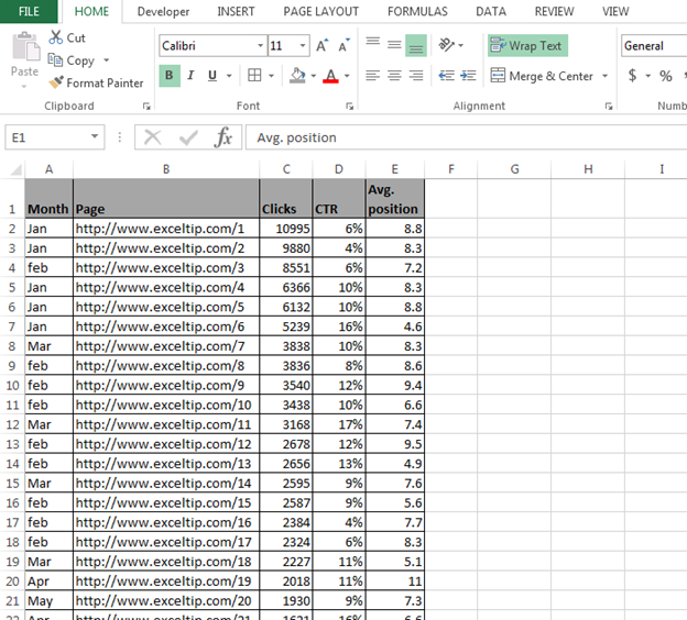
If we want to see the data of Jan month, then we need to put the filter on Jan month. To put the filter through VBA, follow below given steps:-
- Open VBA Page press the key Alt+F11.
- Insert a module.
- Write the below mentioned code:
Sub Filterindata()
Range(«A1″).AutoFilter Field:=1, Criteria1:=»Jan»
End Sub
Code Explanation:- Firstly, we have to select the range of data where we want to put the filter and then we need to define the criteria.
To run the macro, press the key F5, and data will get filtered and we can see only Jan data.

How to put the filter for bottom 10 items?
To understand how to put the filter for bottom 10 items, let’s take an example:-
We have data in range A1:E35 in which column A contains Month, column B Page, column C Clicks, Column D CTR and column E contains average position.

If we want to see the bottom 10 clicks in the data, then we need to follow below given steps:-
- Open VBA Page press the key Alt+F11.
- Insert a module.
- Write the below mentioned code:
Sub filterbottom10()
Range(«A1″).AutoFilter Field:=3, Criteria1:=»10», Operator:=xlBottom10Items
End Sub
Code Explanation:- First, we have to select the range of data where we want to put the filter and then we need to define the criteria to filter the data of bottom 10 items.
To run the macro, press the key F5, and data will get filtered and we can see only bottom10 click’s data.
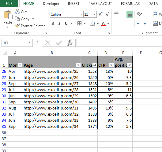
How to put the filter for bottom 10 percent of data?
To understand how to put the filter for bottom 10 percent of data, let’s take an example:-
We have data in range A1:E35 in which column A contains Month, column B Page, column C Clicks, Column D CTR and column E contains average position.
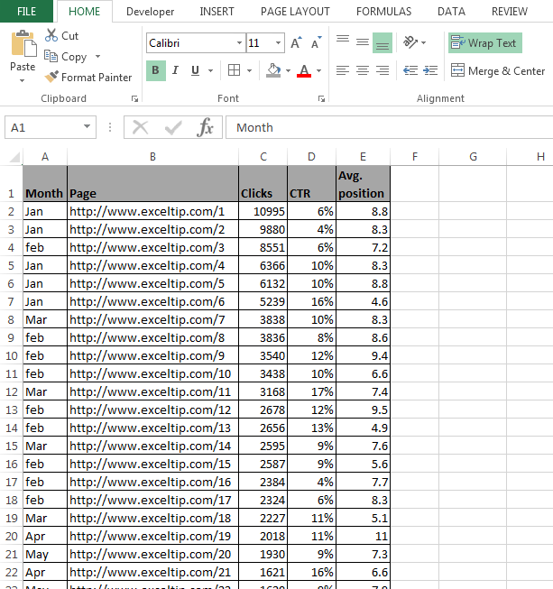
If we want to see the bottom 10 percent data, then we need to follow below given steps:-
- Open VBA Page and press the key Alt+F11.
- Insert a module.
- Write the below mentioned code:
Sub Filterbottom10percent()
Range(«A1″).AutoFilter Field:=3, Criteria1:=»10», Operator:=xlBottom10Percent
End Sub
Code Explanation:- First, we have to select the range of data where we want to put the filter and then we need to define the criteria to filter the data of bottom 10 percent.
To run the macro, press the key F5, and data will get filtered and we can see only bottom10 percent data.
How to put the filter for bottom X number of Items of data?
To understand how to put the filter for bottom X numbers, let’s take an example:-
We have data in range A1:E35 in which column A contains Month, column B Page, column C Clicks, Column D CTR and column E contains average position.

If we want to see the bottom x number of data, then we need to follow below given steps:-
- Open VBA Page press the key Alt+F11.
- Insert a module.
- Write the below mentioned code:
Sub Filterbottomxnumber()
Range(«A1″).AutoFilter Field:=3, Criteria1:=»5», Operator:=xlBottom10Items
End Sub
Code Explanation:- First we have select the range of data where we want to put the filter and then we gave the criteria to filter the 5 numbers of bottom 10 numbers.
To run the macro press the key F5, data will get filtered and we can see only bottom 10 click’s data.
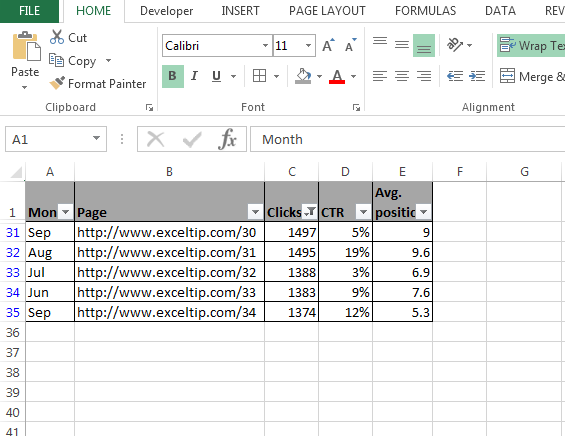
How to put the filter for bottom x percent of data?
To understand that how to put the filter for bottom x percent of data, let’s take an example:-
We have data in range A1:E35, in which column A contains Month, column B Page, column C Clicks, Column D CTR and column E contains average position.

If we want to see the bottom x percent data, then we need to follow below given steps:-
- Open VBA Page press the key Alt+F11.
- Insert a module.
- Write the below mentioned code:
Sub Filterbottomxpercent()
Range(«A1″).AutoFilter Field:=3, Criteria1:=»5», Operator:=xlBottom10Percent
End Sub
Code Explanation:- First we have to select the range of data where we want to put the filter and then we need to define the criteria to filter the data of bottom x percent.
To run the macro, press the key F5, and data will get filtered and we can see only bottom 10 Percent data.
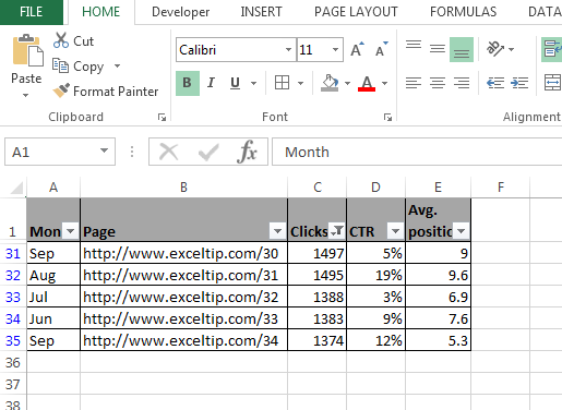
How to put the filter for specific text?
To understand how to put the filter for specific, let’s take an example:-
We have data in range A1:E35 in which column A contains Month, column B Page, column C Clicks, Column D CTR and column E contains average position.

If we want to see the specific data only in column B, then we need to follow below given steps:-
- Open VBA Page and press the key Alt+F11.
- Insert a module.
- Write the below mentioned code:
Sub Specificdata()
Range(«A1″).AutoFilter Field:=2, Criteria1:=»*Exceltip*»
End Sub
Code Explanation:- First we have select the range of data where we will define the column B in Field as 2 and then we will define that which data we want to see.
To run the macro press the key F5, data will get filtered and we can see only Exceltip’s data will appear.
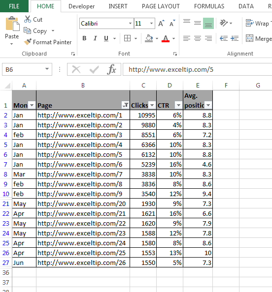
How to put the filter for multiple criteria?
To understand how to put the filter specifically, let’s take an example:-
We have data in range A1:E35 in which column A contains Month, column B Page, column C Clicks, Column D CTR and column E contains average position.

If we want to see the data for Jan and Mar month, then we need to follow below given steps:-
- Open VBA Page press the key Alt+F11.
- Insert a module.
- Write the below mentioned code:
Sub Multipledata()
Range(«A1:E1″).AutoFilter field:=1, Criteria1:=»Jan», Operator:=xlAnd, Criteria2:=»Mar»
End Sub
Code Explanation:- First we have to select the range of data where we will define the column A in Field as 1 and then we will define the both criteria.
To run the macro, press the key F5, and data will get filtered and we can see only Jan and Mar data will appear.
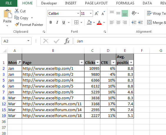
How to put the filter to display the records that contain a value between 2 values?
To understand how to put the filter for multiple criteria, let’s take an example:-
We have data in range A1:E35 in which column A contains Month, column B Page, column C Clicks, Column D CTR and column E contains average position.

If we want to put the filter as per the criteria how many numbers we have under the clicks of 5000 to 10000 , follow below given steps:-
- Open VBA Page and press the key Alt+F11.
- Insert a module.
- Write the below mentioned code:
Sub MultipleCriteria()
Range(«A1:E1″).AutoFilter field:=3, Criteria1:=»>5000″, Operator:=xlAnd, Criteria2:=»<10000″
End Sub
Code Explanation: — First we have to select the range of data where we will define the criteria in column C by using operator function.
To run the macro, press the key F5, and data will get filtered and we can see the data as per the clicks which is more than 5000 and less than 10000.
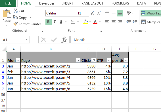
How to put the filter for multiple criteria in multiple columns?
To understand how to put the filter for multiple criteria in multiple columns, let’s take an example:-
We have data in range A1:E35 in which column A contains Month, column B Page, column C Clicks, Column D CTR and column E contains average position.

If we want to put the filter in Jan month to see that how many links are there in excel tips So we have to put the filter in Column A and B, follow below given steps:-
- Open VBA Page press the key Alt+F11.
- Insert a module.
- Write the below mentioned code:
Sub MultipleFields()
Range(«A1:E1″).AutoFilter field:=1, Criteria1:=»Jan»
Range(«A1:E1″).AutoFilter field:=2, Criteria1:=»*Exceltip*»
End Sub
Code Explanation: — Firstly, we have to select the range of data where we want to put the filter and then we will have to define the criteria 2 times to achieve the target.
To run the macro, press the key F5, and data will get filtered and we can see how many links belong to Exceltip in the data of Jan month.

How to filter the data without applying the filter arrow?
To understand how to filter the data without applying the filter in column, let’s take an example:-
We have data in range A1:E35 in which column A contains Month, column B Page, column C Clicks, Column D CTR and column E contains average position.

If we want to put the filter for in Jan month and hide the filter arrow in the field, follow below given steps:-
- Open VBA Page press the key Alt+F11.
- Insert a module.
- Write the below mentioned code:
Sub HideFilter()
Range(«A1″).AutoFilter field:=1, Criteria1:=»Jan», visibledropdown:=False
End Sub
Code Explanation: — First, we have to select the range of data where we want to put the filter and then we need to make sure that filter should not be visible.
To run the macro, press the key F5, and data will get filtered. Now, we can see the data in Jan month’s data only but the filter arrow will not appear in month’s column.
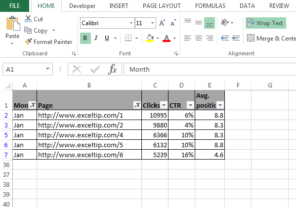
How to filter the data for displaying the 1 0r 2 Possible values?
To understand how to filter the data to display the 1 or 2 possible values, let’s take an example:-
We have data in range A1:E35 in which column A contains Month, column B Page, column C Clicks, Column D CTR and column E contains average position.

If we want to put the filter in Jan month and hide the filter arrow in the field, we need to follow below given steps:-
- Open VBA Page press the key Alt+F11.
- Insert a module.
- Write the below mentioned code:
Sub HideFilter()
Range(«A1″).AutoFilter field:=1, Criteria1:=»Jan», visibledropdown:=False
End Sub
Code Explanation: — Firstly, we have to select the range of data where we want to put the filter and then we will make sure that filter should not be visible.
To run the macro, press the key F5, and data will get filtered. Now, we can see the data in Jan month’s data and Feb month’s data.

How to put the filter for top 10 items?
To understand how to put the filter for top 10 items, let’s take an example:-
We have data in range A1:E35 in which column A contains Month, column B Page, column C Clicks, Column D CTR and column E contains average position.

If we want to see the top 10 clicks in the data, then we need to follow below given steps:-
- Open VBA Page and press the key Alt+F11.
- Insert a module.
- Write the below mentioned code:
Sub filtertop10()
Range(«A1″).AutoFilter Field:=3, Criteria1:=»10», Operator:=xlTop10Items
End Sub
Code Explanation- Firstly, we have to select the range of data where we want to put the filter and then we need to define the criteria to filter the data from top 10 items.
To run the macro, press the key F5, and data will get filtered and we can see only top 10 click’s data.
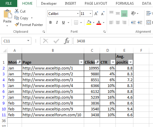
How to put the filter for top 10 percent of data?
To understand how to put the filter for top 10 percent of data, let’s take an example:-
We have data in range A1:E35 in which column A contains Month, column B Page, column C Clicks, Column D CTR and column E contains average position.

If we want to see the top 10 percent data, then we need to follow below given steps:-
- Open VBA Page press the key Alt+F11.
- Insert a module.
- Write the below mentioned code:
Sub Filtertop10percent()
Range(«A1″).AutoFilter Field:=3, Criteria1:=»10», Operator:=xlTop10Percent
End Sub
Code Explanation:- First we have to select the range of data where we want to put the filter and then we need to define the criteria to filter the data from top 10 percent.
To run the macro, press the key F5, and data will get filtered. Now, we can see only top 10 percent data.
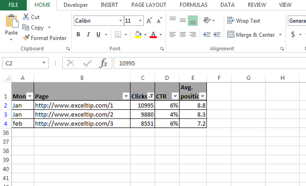
How to remove the filter?
To understand how to remove the filter, follow below given steps:-
- Open VBA Page press the key Alt+F11.
- Insert a module.
- Write the below mentioned code:
Sub removefilter()
Worksheets(«Sheet1»).ShowAllData
End Sub
To run the macro press the key F5, all data will get show but filter arrow will not be remove.
This is all about how we can put the filters through VBA in Microsoft Excel.
![]()
Working with large datasets that contain rows after rows of data can be quite painful.
In such cases, looking for data that match particular criteria can be like looking for a needle in a haystack.
Thankfully, Excel provides some features that let you hide certain rows based on the cell value so that you only see the rows that you want to see. There are two ways to do this:
- Using filters
- Using VBA
In this tutorial, we will discuss both methods, and you can pick the method you feel most comfortable with.
Using Filters to Hide Rows based on Cell Value
Let us say you have the dataset shown below, and you want to see data about only those employees who are still in service.

This is really easy to do using filters. Here are the steps you need to follow:
- Select the working area of your dataset.
- From the Data tab, select the Filter button. You will find it in the ‘Sort and Filter’ group.

- You should now see a small arrow button on every cell of the header row.

- These buttons are meant to help you filter your cells. You can click on any arrow to choose a filter for the corresponding column.
- In this example, we want to filter out the rows that contain the Employment status = “In service”. So, select the arrow next to the Employment Status header.
- Uncheck the boxes next to all the statuses, except “In service”. You can simply uncheck “Select All” to quickly uncheck everything and then just select “In service”.

- Click OK.


You should now be able to see only the rows with Employment Status=”In service”. All other rows should now be hidden.

Note: To unhide the hidden cells, simply click on the Filter button again.
Using VBA to Hide Rows based on Cell Value
The second method requires a little coding. If you are accustomed to using macros and a little coding using VBA, then you get much more scope and flexibility to manipulate your data to behave exactly the way you want.
Writing the VBA Code
The following code will help you display only the rows that contain information about employees who are ‘In service’ and will hide all other rows:
Sub HideRows()
StartRow = 2
EndRow = 19
ColNum = 3
For i = StartRow To EndRow
If Cells(i, ColNum).Value <> "In service" Then
Cells(i, ColNum).EntireRow.Hidden = True
Else
Cells(i, ColNum).EntireRow.Hidden = False
End If
Next i
End Sub
The macro loops through each cell of column C and hide the rows that do not contain the value “In service”. It should essentially analyze each cell from rows 2 to 19 and adjust the ‘Hidden’ attribute of the row that you want to hide.
To enter the above code, copy it and paste it into your developer window. Here’s how:
- From the Developer menu ribbon, select Visual Basic.

- Once your VBA window opens, you will see all your files and folders in the Project Explorer on the left side. If you don’t see Project Explorer, click on View->Project Explorer.

- Make sure ‘ThisWorkbook’ is selected under the VBA project with the same name as your Excel workbook.
- Click Insert->Module. You should see a new module window open up.

- Now you can start coding. Copy the above lines of code and paste them into the new module window.

- In our example, we want to hide the rows that do not contain the value ‘In service’ in column 3. But you can replace the value of ColNum number from “3” in line 4 to the column number containing your criteria values.
- Close the VBA window.


Note: If your dataset covers more than 19 rows, you can change the values of the StartRow and EndRow variables to your required row numbers.
If you can’t see the Developer ribbon, from the File menu, go to Options. Select Customize Ribbon and check the Developer option from Main Tabs.
Finally, Click OK.
Your macro is now ready to use.
Running the Macro
Whenever you need to use the above macro, all you need to do is run it, and here’s how:
- Select the Developer tab
- Click on the Macros button (under the Code group).
- This will open the Macro Window, where you will find the names of all the macros that you have created so far.
- Select the macro (or module) named ‘HideRows’ and click on the Run button.


You should see all the rows where Employment Status is not ’In service’ hidden.

Explanation of the Code
Here’s a line by line explanation of the above code:
- In line 1 we defined the function name.
Sub HideRows()
- In lines 2, 3 and 4 we defined variables to hold the starting row and ending row of the dataset as well as the index of the criteria column.
StartRow = 2
EndRow = 19
ColNum = 3
- In lines 5 to 11, we looped through each cell in column “3” (or column C) of the Active Worksheet. If a cell does not contain the value “Inservice”, then we set the ‘Hidden’ attribute of the entire row (corresponding to that cell) to True, which means we want to hide the entire corresponding row.
For i = StartRow To EndRow
If Cells(i, ColNum).Value <> "In service" Then
Cells(i, ColNum).EntireRow.Hidden = True
Else
Cells(i, ColNum).EntireRow.Hidden = False
End If
Next i
- Line 12 simply demarcates the end of the HideRows function.
End Sub
In this way, the above code hides all the rows that do not contain the value ‘In service’ in column C.
Un-hiding Columns Based On Cell Value
Now that we have been able to successfully hide unwanted rows, what if we want to see the hidden rows again?
Doing this is quite easy. You only need to make a small change to the HideRows function.
Sub UnhideRows()
StartRow = 2
EndRow = 19
ColNum = 3
For i = StartRow To EndRow
Cells(i, ColNum).EntireRow.Hidden = False
Next i
End Sub
Here, we simply ensured that irrespective of the value, all the rows are displayed (by setting the Hidden property of all rows to False).
You can run this macro in exactly the same way as HideRows.

Hiding Rows Based On Cell Values in Real-Time
In the first example, the columns are hidden only when the macro runs. However, most of the time, we want to hide columns on-the-fly, based on the value in a particular cell.
So, let’s now take a look at another example that demonstrates this. In this example, we have the following dataset:
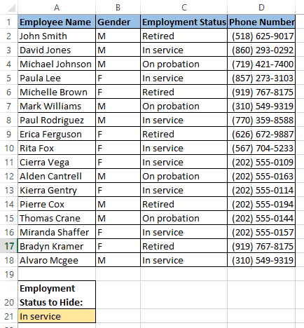
The only difference from the first dataset is that we have a value in cell A21 that will determine which rows should be hidden. So when cell A21 contains the value ‘Retired’ then only the rows containing the Employment Status ‘Retired’ are hidden.
Similarly, when cell A21 contains the value ‘On probation’ then only the rows containing the Employment Status ‘On probation’ are hidden.
When there is nothing in cell A21, we want all rows to be displayed.
We want this to happen in real-time, every time the value in cell A21 changes. For this, we need to make use of Excel’s Worksheet_SelectionChange function.
The Worksheet_SelectionChange Event
The Worksheet_SelectionChange procedure is an Excel built-in VBA event
It comes pre-installed with the worksheet and is called whenever a user selects a cell and then changes his/her selection to some other cell.
Since this function comes pre-installed with the worksheet, you need to place it in the code module of the correct sheet so that you can use it.
In our code, we are going to put all our lines inside this function, so that they get executed whenever the user changes the value in A21 and then selects some other cell.
Writing the VBA Code
Here’s the code that we are going to use:
StartRow = 2
EndRow = 19
ColNum = 3
For i = StartRow To EndRow
If Cells(i, ColNum).Value = Range("A21").Value Then
Cells(i, ColNum).EntireRow.Hidden = True
Else
Cells(i, ColNum).EntireRow.Hidden = False
End If
Next i
To enter the above code, you need to copy it and paste it in your developer window, inside your worksheet’s Worksheet_SelectionChange procedure. Here’s how:
- From the Developer menu ribbon, select Visual Basic.
- Once your VBA window opens, you will see all your project files and folders in the Project Explorer on the left side.
- In the Project Explorer, double click on the name of your worksheet, under the VBA project with the same name as your Excel workbook. In our example, we are working with Sheet1.
- This will open up a new module window for your selected sheet.
- Click on the dropdown arrow on the left of the window. You should see an option that says ‘Worksheet’.

- Click on the ‘Worksheet’ option. By default, you will see the Worksheet_SelectionChange procedure created for you in the module window.
- Now you can start coding. Copy the above lines of code and paste them into the Worksheet_SelectionChange procedure, right after the line: Private Sub Worksheet_SelectionChange(ByVal Target As Range).

- Close the VBA window.


Running the Macro
The Worksheet_SelectionChange procedure starts running as soon as you are done coding. So you don’t need to explicitly run the macro for it to start working.
Try typing the ‘Retired’ in the cell A21, then clicking any other cell. You should find all rows containing the value ‘Retired’ in column C disappear.

Now try replacing the value in cell A21 to ‘On probation’, then clicking any other cell. You should find all rows containing the value ‘On probation’ in column C disappear.

Now try removing the value in cell A21 and leaving it empty. Then click on any other cell. You should find both rows become visible again.

This means the code is working in real-time when changes are made to cell B20.
Explanation of the Code
Let us take a few minutes to understand this code now.
- Lines 1, 2, and 3 define variables to hold the starting row and ending row of the dataset as well as the index of the criteria column. You can change the values according to your requirement.
StartRow = 2
EndRow = 19
ColNum = 3
- Lines 4 to 10, loop through each cell in column “3” (or column C) of the worksheet. If the cell contains the value in cell A21, then we set the ‘Hidden’ attribute of the entire row (corresponding to that cell) to True, which means we want to hide the entire corresponding row.
For i = StartRow To EndRow
If Cells(i, ColNum).Value = Range("A21").Value Then
Cells(i, ColNum).EntireRow.Hidden = True
Else
Cells(i, ColNum).EntireRow.Hidden = False
End If
Next i
In this way, the above code hides the rows of the dataset depending on the value in cell A21. If A21 does not contain any value then the code displays all rows.
In this tutorial, I showed you how you can use Filters as well as Excel VBA to hide rows based on a cell value.
I did this with the help of two simple examples – one that removes required rows only when the macro is explicitly run and another that works in real-time.
I hope that we have been successful in helping you understand the concept behind the code so that you can customize it and use it in your own applications.
Other Excel tutorials you may also like:
- How to Hide Columns Based On Cell Value in Excel
- How to Delete Filtered Rows in Excel (with and without VBA)
- How to Highlight Every Other Row in Excel (Conditional Formatting & VBA)
- How to Unhide All Rows in Excel with VBA
- How to Set a Row to Print on Every Page in Excel
- How to Paste in a Filtered Column Skipping the Hidden Cells
- How to Select Multiple Rows in Excel
- How to Select Rows with Specific Text in Excel
- How to Move Row to Another Sheet Based On Cell Value in Excel?
- How to Compare Two Cells in Excel?
Lets say i have a named range in excel. It has links to recipes in column A. Adjacent columns have some more information on the recipe.
For instance column B has ‘Ingredients’, column C has ‘Kitchen utensils needed’, column D has ‘Course’.
In all cells of columns B and further there may be multiple entries, in random order, separated by comma’s. E.g. for apple pie the ingredients would be ‘Apple, butter, egg, sugar’. Kitchen utensils could ‘oven, pie-container, mixing-machine’
I made some multiple select listboxes in which all possible ingredients are listed, all possible utensils are listed, etc. I want to use the listboxes to filter out the appropriate recipes.
Now the autofilter can only filter up to two words at the same time for one specific column. I want to be able to look up any amounts of ingredients at the same time. All recipes having any of the selected ingredients must show up, even if i select 10 ingredients.
There is also the advanced filter, however because i have multiple columns (10 for the actual data which is not recipes) and want to be able to select up to 10 (more or less) search values per column, the amount of combinations that i need to supply for the advanced filter quickly grows out of control.
Any thoughts on how to achieve this in VBA?
So all rows where Column A contains (x or y or z or …) AND Column B contains (f or g or h or …) AND column C contains (q or p or r or …), etc.
It’s quite easily written down in one sentence here, but I’m a bit lost at making the translation to VBA code for the filtering. I do have the selected values of the listboxes in a dict.