Filter numbers in excel - Word и Excel - помощь в работе с программами

Use AutoFilter or built-in comparison operators like «greater than» and “top 10” in Excel to show the data you want and hide the rest. Once you filter data in a range of cells or table, you can either reapply a filter to get up-to-date results, or clear a filter to redisplay all of the data.

Use filters to temporarily hide some of the data in a table, so you can focus on the data you want to see.

Filter a range of data

Select any cell within the range.
Select Data > Filter.
Select the column header arrow .
Select Text Filters or Number Filters, and then select a comparison, like Between.
Enter the filter criteria and select OK.

Filter data in a table

When you put your data in a table, filter controls are automatically added to the table headers.

Select the column header arrow for the column you want to filter.
Uncheck (Select All) and select the boxes you want to show.
Click OK.

The column header arrow changes to a Filter icon. Select this icon to change or clear the filter.

Filter data in a table

When you put your data in a table, filtering controls are added to the table headers automatically.

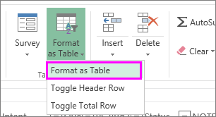
Select the data you want to filter. On the Home tab, click Format as Table, and then pick Format as Table.
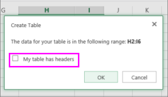
In the Create Table dialog box, you can choose whether your table has headers.
- Select My table has headers to turn the top row of your data into table headers. The data in this row won’t be filtered.
- Don’t select the check box if you want Excel for the web to add placeholder headers (that you can rename) above your table data.
Click OK.
To apply a filter, click the arrow in the column header, and pick a filter option.

Filter a range of data

If you don’t want to format your data as a table, you can also apply filters to a range of data.

Select the data you want to filter. For best results, the columns should have headings.
On the Data tab, choose Filter.

Filtering options for tables or ranges

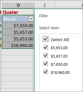
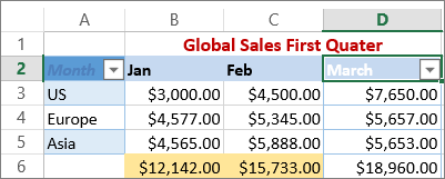
You can either apply a general Filter option or a custom filter specific to the data type. For example, when filtering numbers, you’ll see Number Filters, for dates you’ll see Date Filters, and for text you’ll see Text Filters. The general filter option lets you select the data you want to see from a list of existing data like this:

Number Filters lets you apply a custom filter:

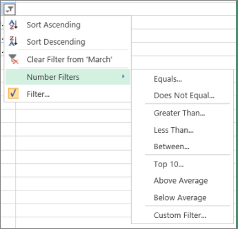
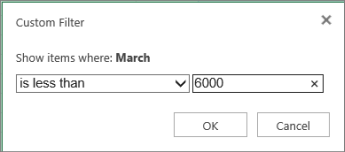
In this example, if you want to see the regions that had sales below $6,000 in March, you can apply a custom filter:

Here’s how:

Click the filter arrow next to March > Number Filters > Less Than and enter 6000.
Click OK.

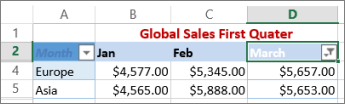
Excel for the web applies the filter and shows only the regions with sales below $6000.

You can apply custom Date Filters and Text Filters in a similar manner.

To clear a filter from a column

Click the Filter button next to the column heading, and then click Clear Filter from <«Column Name»>.

To remove all the filters from a table or range

Select any cell inside your table or range and, on the Data tab, click the Filter button.

This will remove the filters from all the columns in your table or range and show all your data.

Click a cell in the range or table that you want to filter.
On the Data tab, click Filter.
Click the arrow in the column that contains the content that you want to filter.
Under Filter, click Choose One, and then enter your filter criteria.

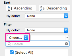
Notes:

You can apply filters to only one range of cells on a sheet at a time.
When you apply a filter to a column, the only filters available for other columns are the values visible in the currently filtered range.
Only the first 10,000 unique entries in a list appear in the filter window.

Click a cell in the range or table that you want to filter.
On the Data tab, click Filter.
Click the arrow in the column that contains the content that you want to filter.
Under Filter, click Choose One, and then enter your filter criteria.
In the box next to the pop-up menu, enter the number that you want to use.
Depending on your choice, you may be offered additional criteria to select:

Notes:

You can apply filters to only one range of cells on a sheet at a time.
When you apply a filter to a column, the only filters available for other columns are the values visible in the currently filtered range.
Only the first 10,000 unique entries in a list appear in the filter window.
Instead of filtering, you can use conditional formatting to make the top or bottom numbers stand out clearly in your data.

You can quickly filter data based on visual criteria, such as font color, cell color, or icon sets. And you can filter whether you have formatted cells, applied cell styles, or used conditional formatting.

In a range of cells or a table column, click a cell that contains the cell color, font color, or icon that you want to filter by.
On the Data tab, click Filter .
Click the arrow in the column that contains the content that you want to filter.
Under Filter, in the By color pop-up menu, select Cell Color, Font Color, or Cell Icon, and then click a color.

This option is available only if the column that you want to filter contains a blank cell.

Click a cell in the range or table that you want to filter.
On the Data toolbar, click Filter.
Click the arrow in the column that contains the content that you want to filter.
In the (Select All) area, scroll down and select the (Blanks) check box.
Notes:
- You can apply filters to only one range of cells on a sheet at a time.
- When you apply a filter to a column, the only filters available for other columns are the values visible in the currently filtered range.
- Only the first 10,000 unique entries in a list appear in the filter window.

Click a cell in the range or table that you want to filter.
On the Data tab, click Filter .
Click the arrow in the column that contains the content that you want to filter.

Under Filter, click Choose One, and then in the pop-up menu, do one of the following:

To filter the range for	Click
Rows that contain specific text	Contains or Equals.
Rows that do not contain specific text	Does Not Contain or Does Not Equal.

In the box next to the pop-up menu, enter the text that you want to use.

Depending on your choice, you may be offered additional criteria to select:

To	Click
Filter the table column or selection so that both criteria must be true	And.
Filter the table column or selection so that either or both criteria can be true	Or.

Click a cell in the range or table that you want to filter.
On the Data toolbar, click Filter .
Click the arrow in the column that contains the content that you want to filter.

Under Filter, click Choose One, and then in the pop-up menu, do one of the following:

To filter for	Click
The beginning of a line of text	Begins With.
The end of a line of text	Ends With.
Cells that contain text but do not begin with letters	Does Not Begin With.
Cells that contain text but do not end with letters	Does Not End With.

In the box next to the pop-up menu, enter the text that you want to use.

Depending on your choice, you may be offered additional criteria to select:

To	Click
Filter the table column or selection so that both criteria must be true	And.
Filter the table column or selection so that either or both criteria can be true	Or.

Wildcard characters can be used to help you build criteria.

Click a cell in the range or table that you want to filter.
On the Data toolbar, click Filter.
Click the arrow in the column that contains the content that you want to filter.
Under Filter, click Choose One, and select any option.
In the text box, type your criteria and include a wildcard character.

For example, if you wanted your filter to catch both the word «seat» and «seam», type sea?.

Do one of the following:

Use	To find
? (question mark)	Any single character For example, sm?th finds «smith» and «smyth»
* (asterisk)	Any number of characters For example, *east finds «Northeast» and «Southeast»
~ (tilde)	A question mark or an asterisk For example, there~? finds «there?»

Use

To find

? (question mark)

Any single character

For example, sm?th finds «smith» and «smyth»

* (asterisk)

Any number of characters

For example, *east finds «Northeast» and «Southeast»

~ (tilde)

A question mark or an asterisk

For example, there~? finds «there?»

Do any of the following:

To	Do this
Remove specific filter criteria for a filter	Click the arrow in a column that includes a filter, and then click Clear Filter.
Remove all filters that are applied to a range or table	Select the columns of the range or table that have filters applied, and then on the Data tab, click Filter.
Remove filter arrows from or reapply filter arrows to a range or table	Select the columns of the range or table that have filters applied, and then on the Data tab, click Filter.

When you filter data, only the data that meets your criteria appears. The data that doesn’t meet that criteria is hidden. After you filter data, you can copy, find, edit, format, chart, and print the subset of filtered data.

Table with Top 4 Items filter applied

Filters are additive. This means that each additional filter is based on the current filter and further reduces the subset of data. You can make complex filters by filtering on more than one value, more than one format, or more than one criteria. For example, you can filter on all numbers greater than 5 that are also below average. But some filters (top and bottom ten, above and below average) are based on the original range of cells. For example, when you filter the top ten values, you’ll see the top ten values of the whole list, not the top ten values of the subset of the last filter.

In Excel, you can create three kinds of filters: by values, by a format, or by criteria. But each of these filter types is mutually exclusive. For example, you can filter by cell color or by a list of numbers, but not by both. You can filter by icon or by a custom filter, but not by both.

Filters hide extraneous data. In this manner, you can concentrate on just what you want to see. In contrast, when you sort data, the data is rearranged into some order. For more information about sorting, see Sort a list of data.

When you filter, consider the following guidelines:

Only the first 10,000 unique entries in a list appear in the filter window.
You can filter by more than one column. When you apply a filter to a column, the only filters available for other columns are the values visible in the currently filtered range.
You can apply filters to only one range of cells on a sheet at a time.

Note: When you use Find to search filtered data, only the data that is displayed is searched; data that is not displayed is not searched. To search all the data, clear all filters.

Need more help?

You can always ask an expert in the Excel Tech Community or get support in the Answers community.

Источник

На чтение 4 мин. Просмотров 4.4k.

Итог: узнайте, как применять числовые фильтры с VBA. Статья включает примеры фильтрации для диапазона между двумя числами: ТОП 10, больше/меньше среднего и т.д.

Уровень мастерства: Средний

Содержание

Скачать файл
Числовые фильтры в Excel
Образцы кода VBA для числовых фильтров
Фильтры и типы данных

Скачать файл

Файл Excel, содержащий код, можно скачать ниже. Этот файл содержит код для фильтрации различных типов данных и типов фильтров. Пожалуйста, ознакомьтесь с моей статьей Фильтрация сводной таблицы или среза по самой последней дате или периоду для более подробной информации.

VBA AutoFilters Guide.xlsm (100.5 KB)

Числовые фильтры в Excel

При фильтрации столбца, содержащего числа, мы можем выбрать
элементы из списка раскрывающегося меню фильтра.

Тем не менее, обычно проще использовать параметры в подменю Number Filters для создания пользовательского фильтра. Это дает нам возможности для критериев фильтрации, которые равны, не равны, больше, меньше, меньше или равны, ТОП 10 и выше/ниже среднего.

Следующий макрос содержит примеры фильтрации чисел. Пожалуйста, ознакомьтесь с моей статьей Фильтрация сводной таблицы или среза по самой последней дате или периоду для получения более подробной информации о том, как использовать метод AutoFilter и его параметры.

При применении фильтра для одного числа нам нужно
использовать форматирование чисел, которое применяется в столбце. Это странная
причуда VBA, которая может привести к неточным результатам, если вы не знаете
правила. В приведенном ниже коде есть пример.

Образцы кода VBA для числовых фильтров

Код в поле ниже можно скопировать / вставить в VB Editor.

Sub AutoFilter_Number_Examples()
' Примеры фильтрации столбцов с помощью NUMBERS
 
Dim lo As ListObject
Dim iCol As Long
  ' Установить ссылку на первую таблицу на листе
  Set lo = Sheet1.ListObjects(1)
  
  ' Установить поле фильтра
   iCol = lo.ListColumns("Revenue").Index
   
  ' Очистить фильтры
  lo.AutoFilter.ShowAllData

  With lo.Range
  
    ' Одно число - используйте форматирование, которое видно в
    ' раскрывающемся меню фильтра
    .AutoFilter Field:=iCol, Criteria1:="$2,955.25"
    
    ' Не равно - не требует форматирования чисел для соответствия
    .AutoFilter Field:=iCol, Criteria1:="<>2955.25"
    
    ' Больше или меньше, чем число
    ' (оператор сравнения <> = перед числом в Criteria1)
    .AutoFilter Field:=iCol, Criteria1:="<4000"
    
    ' Между 2 числами
    ' (больше или равно 100 и меньше 4000)
    .AutoFilter Field:=iCol, _
                Criteria1:=">=100", _
                Operator:=xlAnd, _
                Criteria2:="<4000"
    
    ' Вне диапазона (меньше 100 ИЛИ больше 4000)
    .AutoFilter Field:=iCol, _
                Criteria1:="<100", _
                Operator:=xlOr, _
                Criteria2:=">4000"
  
    ' Топ-10 товаров (Критерий1 - количество товаров)
    .AutoFilter Field:=iCol, _
                Criteria1:="10", _
                Operator:=xlTop10Items
    
    ' Нижние 5 пунктов (Критерий1 - количество элементов)
    .AutoFilter Field:=iCol, _
                Criteria1:="5", _
                Operator:=xlBottom10Items
    
    ' Топ 10 процентов (Criteria1 - количество элементов)
    .AutoFilter Field:=iCol, _
                Criteria1:="10", _
                Operator:=xlTop10Percent
    
    ' Нижний 7 процентов
    .AutoFilter Field:=iCol, _
                Criteria1:="7", _
                Operator:=xlBottom10Percent
    
    ' Выше среднего - оператор: = xlFilterDynamic
    .AutoFilter Field:=iCol, _
                Criteria1:=xlFilterAboveAverage, _
                Operator:=xlFilterDynamic
    
    ' Ниже среднего
    .AutoFilter Field:=iCol, _
                Criteria1:=xlFilterBelowAverage, _
                Operator:=xlFilterDynamic
    
  End With
  
End Sub

Фильтры и типы данных

Параметры
раскрывающегося меню фильтра изменяются в зависимости от типа данных в столбце.
У нас есть разные фильтры для текста, чисел, дат и цветов. Это создает МНОГО
различных комбинаций операторов и критериев для каждого типа фильтра.

Я создал отдельные статьи для каждого из этих типов фильтров. Статьи содержат пояснения и примеры кода VBA.

Как очистить фильтры с помощью VBA
Как отфильтровать пустые и непустые клетки
Как фильтровать текст с помощью VBA
Как отфильтровать даты по VBA
Как отфильтровать цвета и значки с помощью VBA

Файл в разделе загрузок выше содержит все эти примеры кода в одном месте. Вы можете добавить его в свою личную книгу макросов и использовать макросы в своих проектах.

Пожалуйста, оставьте
комментарий ниже с любыми вопросами или предложениями. Спасибо!

Источник

Number Filter | Text Filter

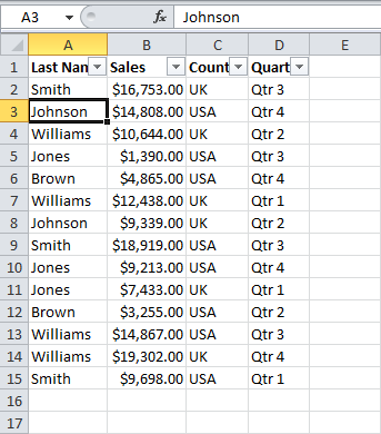
This example teaches you how to apply a number filter and a text filter to only display records that meet certain criteria.

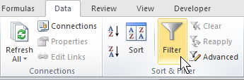
1. Click any single cell inside a data set.

2. On the Data tab, in the Sort & Filter group, click Filter.

Arrows in the column headers appear.

Number Filter

To apply a number filter, execute the following steps.

3. Click the arrow next to Sales.

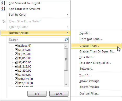
4. Click Number Filters (this option is available because the Sales column contains numeric data) and select Greater Than from the list.

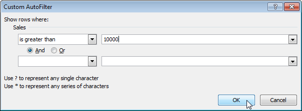
5. Enter 10,000 and click OK.

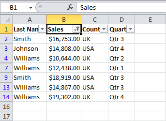
Result. Excel only displays the records where Sales is greater than $10,000.

Note: you can also display records equal to a value, less than a value, between two values, the top x records, records that are above average, etc. The sky is the limit!

Text Filter

To apply a text filter, execute the following steps.

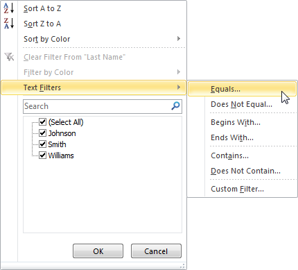
3. Click the arrow next to Last Name.

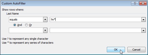
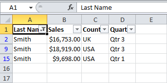
4. Click Text Filters (this option is available because the Last Name column contains text data) and select Equals from the list.

5. Enter ?m* and click OK.

Note: A question mark (?) matches exactly one character. An asterisk (*) matches a series of zero or more characters.

Result. Excel only displays the records where the second character of Last Name equals m.

Note: you can also display records that begin with a specific character, end with a specific character, contain or do not contain a specific character, etc. The sky is the limit!

Источник

Bottom line: Learn the correct way to filter out zeros and numbers with the filter drop-down menus in Excel, and avoid embarrassing mistakes.

Skill level: Intermediate

The image above shows a way to filter out numbers or zeros using the check boxes in the filter drop-down list. This way of applying number filters has gotten me in trouble. I have seen others make this common mistake too, and don’t want it to happen to you. 🙂

Download Example File

Download the example file to follow along.

The Easy, But INCORRECT Way to Filter Out Zeros

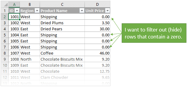
Often times we are working with a list or data set that contains a lot of zeros in a column. We might want to filter these zeros out to shorten the list, so that we only see numbers that are greater than or less than zero.

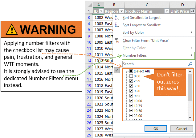
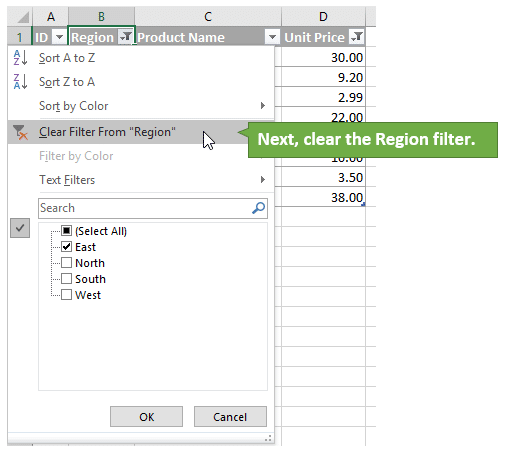
One easy way to do this is to uncheck the zero (0) item in the filter drop-down box.

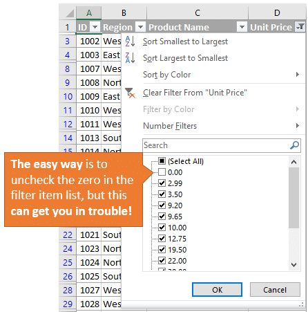
This does work, and will filter out (hide) the rows that contain zeros in the cells for the column. There won’t be any issues if you only have that one column filtered.

However, problems arise when you have filters applied to more than one column.

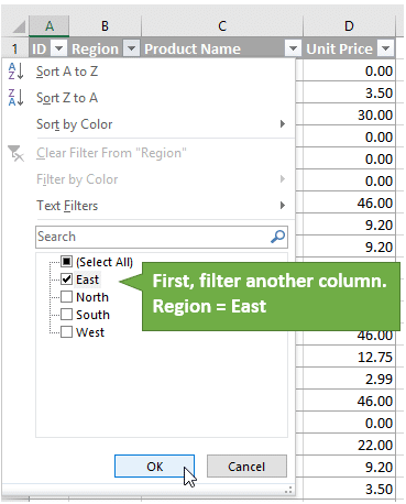
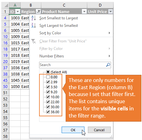
For example, let’s say that we:

First apply a filter to column B for the East Region.
Then apply a filter to column D to exclude zeros by unchecking the zero item check box.

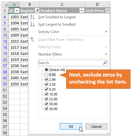
Everything is fine at this point.

We are seeing rows for the East Region where the Unit Price is not zero. This is our filter context.

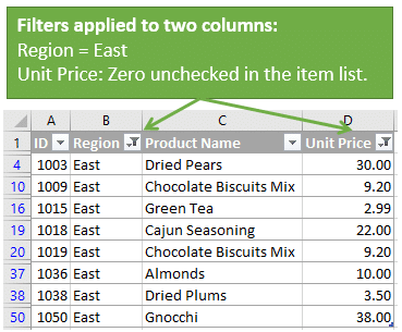
Now, I want to clear the Region filter to view all Regions.

I assume that I should see rows for all Regions where the Unit Price is not zero.

WRONG!!!

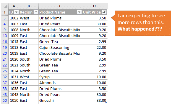
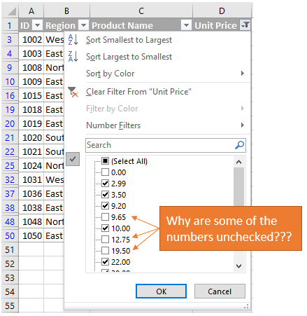
If we look at the filter drop-down for the Unit Price we can see that there are some amounts that are unchecked. That means that these rows are hidden, even though the amount is not zero.

What’s going on???

The Filter Drop-down List Checkboxes Explained

The filter list in the filter drop-down menu displays a list of unique items for that column (field). We can check or uncheck items in the list to apply filters and hide rows in the range/table.

When we uncheck one or more items, the filter creates a filter criteria to apply to the list. This filter criteria is a list of all the checked items. This is important.

The filter criteria does NOT consider the unchecked items. Even if you have one item unchecked, and 1,000 items checked, the filter criteria will be for the 1,000 checked items.

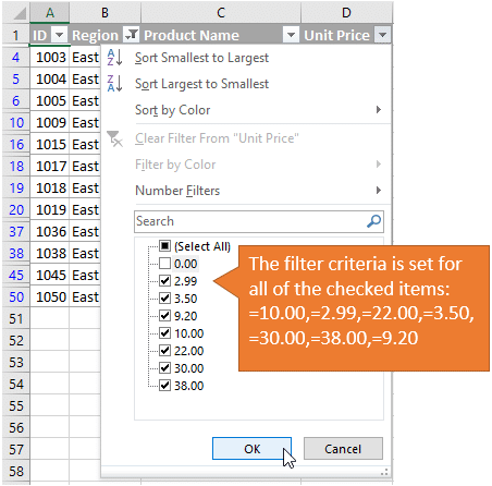
In the example above, when I unchecked the zero in column D, the filter criteria became.

=10.00,=2.99,=22.00,=3.50,=30.00,=38.00,=9.20

I used a little VBA code to get the filter criteria.

Even though I meant to apply a filter to exclude zero, I actually applied a filter to include all the other numbers besides zero.

Since I had already applied a filter for the East Region, the Unit Price item list only contained numbers for the visible rows.

When we clear the filter in column B to show all Regions, the filter criteria for column D does NOT change. This means that there is still a filter applied for the numbers that are not zero for the East Region only.

Some of these numbers might also exist in rows for other regions, but overall it just becomes a meaningless mess. 🙂 This can lead to a lot of confusion when you are trying to tie out numbers or validate a summary report calculation.

So let’s take a look at a safer approach.

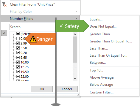
The Correct Way to Filter Numbers

We saw how using the filter list checkboxes can get us in trouble when filtering numbers.

The safest way to filter numbers is by using the Number Filters menu on the filter list drop-down.

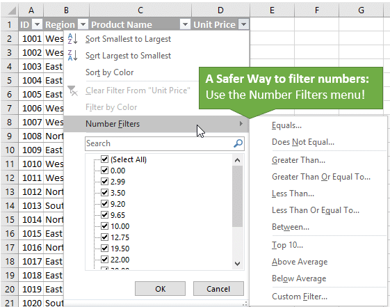
Selecting the Number Filters option will display a sub-menu with different number filter options (Equals, Does Not Equal, Greater Than, Less Than, Top 10, etc.)

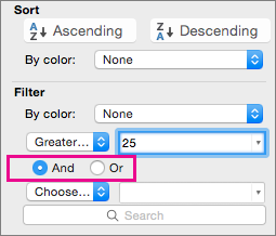
Most of these commands open the Custom AutoFilter menu. This menu allows you to specify two criteria with an AND or OR condition.

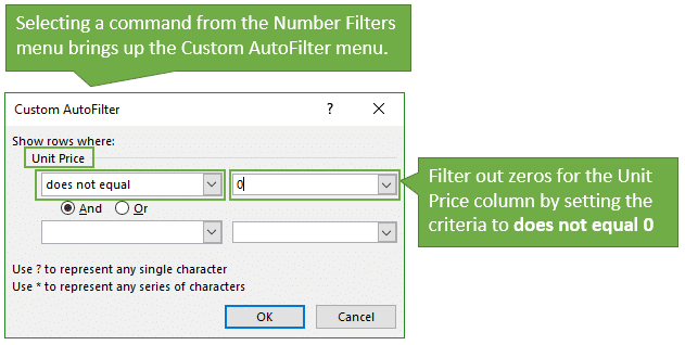
It is easy to create a filter to exclude zeros. We will set the filter criteria to “does not equal”, put a zero in the combobox to the right of the criteria, and press OK.

This sets a number filter with a criteria of “does not equal 0”:

<>0

The less than and greater than symbols together “<>” is the comparison operator for Not Equal, or the opposite of “=”.

This filter criteria helps us avoid the problem we experienced with the filter checkbox list.

Now when we clear or change the Region filter in column B, the number filter in column D will be re-applied to exclude all cells that contain a zero.

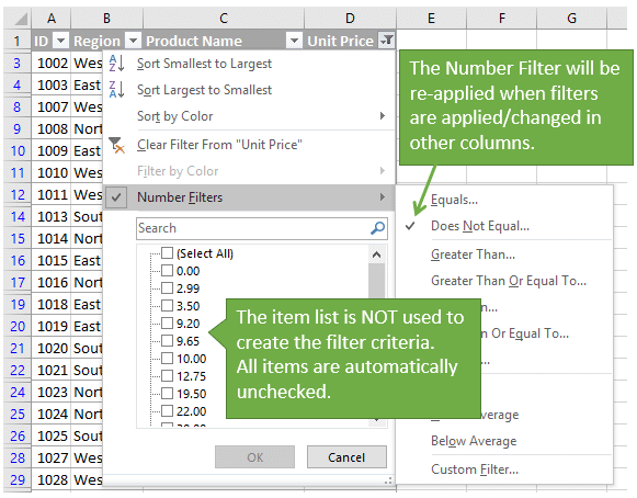
This is what we want. We don’t have to go back to column D and re-select the checkboxes. The number filter will automatically be applied.

Keyboard Shortcuts for the Number Filters

The number filters take a few extra steps to apply, but it is well worth the time and effort if you are filtering multiple columns.

We can also use keyboard shortcuts to quickly apply a filter to exclude zeros.

With the header cell selected (the cell that contains the drop-down icon), press:

Alt+Down Arrow, F, N, 0, Enter

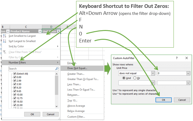
That is the keyboard shortcut to apply the number filter does not equal 0. There are many variations to this keyboard shortcut combination. Each of the underlined letters in the filter drop-down menu is the shortcut key for that menu item.

Checkout my article on 7 keyboard shortcuts for the filter drop-down menus that will save you a lot of time when working with filters. I also explain my favorite shortcut key to put the cursor in the Search box.

Conclusion

As we’ve seen, the filter drop-down item list can get us in trouble. I hope this article helps you avoid some of the mistakes I have made, along with the embarrassment… 🙂

In another article I will follow up with the VBA code and macro to get the filter criteria for the filter range or Table.

Please leave a comment below with any questions. Thanks!

Источник

Перейти к содержанию

На чтение 2 мин Опубликовано 29.09.2015

Числовой фильтр
Текстовый фильтр

Этот пример обучит вас применять числовой и текстовый фильтры так, чтобы отображались только записи, соответствующие определенным критериям.

Кликните по любой ячейке из набора данных.
На вкладке Данные (Data) нажмите кнопку Фильтр (Filter).В заголовках столбцов появятся стрелки.

Числовой фильтр

Чтобы применить числовой фильтр, сделайте следующее:

Нажмите на стрелку в столбце Sales.
Выберите Числовые фильтры (Number Filters). Эта опция доступна, поскольку рассматриваемый столбец содержит числовые данные. В открывшемся списке кликните по пункту Больше (Greater Than).
Введите «10000» и нажмите ОК.

Результат: Excel отображает только те записи, где продажи больше $10000.

Примечание: Ещё можно отобразить только данные, равные какому-либо значению, меньше определенного значения, между двумя значениями, первые n чисел из списка, значения выше среднего и т.д.

Текстовый фильтр

Чтобы применить текстовый фильтр, выполните следующие действия:

Нажмите на стрелку в столбце Last Name.
Выберите Текстовые фильтры (Text Filters). Эта опция доступна, поскольку рассматриваемый столбец содержит текстовые данные. В выпадающем списке кликните по пункту Равно (Equals).
Введите «?m*» и нажмите ОК.

Примечание: Вопросительный знак (?) соответствует ровно одному любому символу. Звездочка (*) соответствует нескольким символам (от нуля и более).

Результат: Excel отображает только те данные, где второй символ равен «m».

Примечание: Ещё можно отобразить данные, которые начинаются с определенного символа, заканчиваются определенным символом, содержат или не содержат определенный символ и т.д.

Оцените качество статьи. Нам важно ваше мнение:

Источник

Filter a range of data

Filter data in a table

Related Topics

Filter data in a table

Filter a range of data

Filtering options for tables or ranges

To clear a filter from a column

To remove all the filters from a table or range

Need more help?

Скачать файл

Числовые фильтры в Excel

Образцы кода VBA для числовых фильтров

Фильтры и типы данных

Number Filter

Text Filter

Download Example File

The Easy, But INCORRECT Way to Filter Out Zeros

The Filter Drop-down List Checkboxes Explained

The Correct Way to Filter Numbers

Keyboard Shortcuts for the Number Filters

Conclusion

Числовой фильтр

Текстовый фильтр