Filter function excel 2016

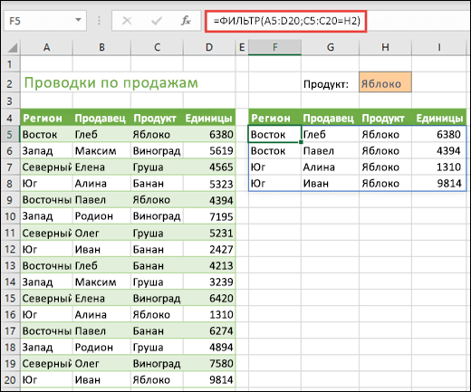
Функция ФИЛЬТР позволяет выполнять фильтрацию диапазона данных на основе условий, которые вы определяете.

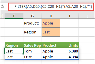
В следующем примере мы использовали формулу =FILTER(A5:D20,C5:C20=H2,»») для возврата всех записей Для Apple, как указано в ячейке H2, и если яблок нет, возвращается пустая строка («»).

Функция ФИЛЬТР фильтрует массив с учетом массива логических значений (ИСТИНА/ЛОЖЬ).

=ФИЛЬТР(массив;включить;[если_пусто])

Аргумент	Описание
массив Обязательный элемент	Массив или диапазон для фильтрации
включить Обязательный элемент	Массив логических переменных с аналогичной высотой или шириной, что и массив.
[если_пусто] Необязательный элемент	Значение, возвращаемое, если все значения во включенном массиве пустые (фильтр не возвращает ничего)

Примечания: 

• Массив может рассматриваться как ряд значений, столбец со значениями или комбинация строк и столбцов значений. В приведенном выше примере массив для нашей формулы ФИЛЬТР представляет собой диапазон A5:D20.

• Функция ФИЛЬТР возвращает массив, который будет переноситься на другие ячейки, если является конечным результатом формулы. Это означает, что Excel будет динамически создавать соответствующий по размеру диапазон массива при нажатии клавиши ВВОД. Если ваши вспомогательные данные хранятся в таблице Excel, тогда массив будет автоматически изменять размер при добавлении и удалении данных из диапазона массива, если вы используете структурированные ссылки. Дополнительные сведения см. в статье о переносе массива.

• Если набор данных потенциально может возвращать пустое значение, используйте третий аргумент ([если_пусто]). В противном случае возникнет ошибка #ВЫЧИС! , так как Excel в настоящее время не поддерживает пустые массивы.

• Если какое-либо значение аргумента include является ошибкой (#N/A, #VALUE и т. д.) или не может быть преобразовано в логическое значение, функция FILTER вернет ошибку.  

• Приложение Excel ограничило поддержку динамических массивов в операциях между книгами, и этот сценарий поддерживается, только если открыты обе книги. Если закрыть исходную книгу, все связанные формулы динамического массива вернут ошибку #ССЫЛКА! после обновления.

Примеры

Функция ФИЛЬТР, используемая для возврата нескольких условий

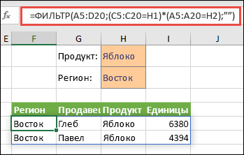
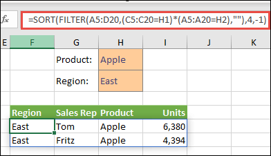
В данном случае мы используем оператор умножения (*) для возврата всех значений в диапазоне массива (A5:D20), содержащих текст «Яблоко» И находящихся в восточном регионе: =ФИЛЬТР(A5:D20;(C5:C20=H1)*(A5:A20=H2);»»).

Функция ФИЛЬТР, используемая для возврата нескольких условий и сортировки

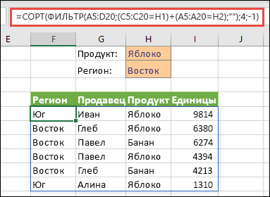
В данном случае мы используем предыдущую функцию ФИЛЬТР с функцией СОРТ для возврата всех значений в диапазоне массива (A5:D20), содержащих текст «Яблоко» И находящихся в восточном регионе, а затем для сортировки единиц в порядке убывания: =СОРТ(ФИЛЬТР(A5:D20;(C5:C20=H1)*(A5:A20=H2);»»);4;-1)

В данном случае мы используем функцию ФИЛЬТР с оператором сложения (+) для возврата всех значений в диапазоне массива (A5:D20), содержащих текст «Яблоко» ИЛИ находящихся в восточном регионе, а затем для сортировки единиц в порядке убывания: =СОРТ(ФИЛЬТР(A5:D20;(C5:C20=H1)+(A5:A20=H2);»»),4;-1).

Обратите внимание на то, что ни одна из функций не требует абсолютных ссылок, так как они находятся только в одной ячейке, а их результаты переносятся в соседние ячейки.

Дополнительные сведения

Вы всегда можете задать вопрос специалисту Excel Tech Community или попросить помощи в сообществе Answers community.

См. также

Функция СЛМАССИВ

Функция ПОСЛЕДОВ

Функция СОРТ

Функция СОРТПО

Функция УНИК

Ошибки #ПЕРЕНОС! в Excel

Динамические массивы и поведение массива с переносом

Оператор неявного пересечения: @

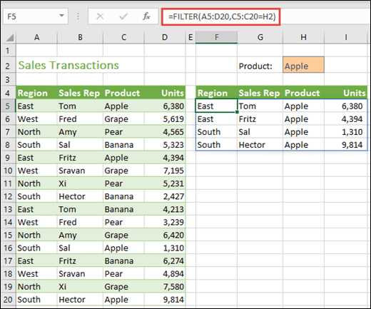
The FILTER function allows you to filter a range of data based on criteria you define.

In the following example we used the formula =FILTER(A5:D20,C5:C20=H2,»») to return all records for Apple, as selected in cell H2, and if there are no apples, return an empty string («»).

The FILTER function filters an array based on a Boolean (True/False) array.

=FILTER(array,include,[if_empty])

Argument	Description
array Required	The array, or range to filter
include Required	A Boolean array whose height or width is the same as the array
[if_empty] Optional	The value to return if all values in the included array are empty (filter returns nothing)

Notes: 

• An array can be thought of as a row of values, a column of values, or a combination of rows and columns of values. In the example above, the source array for our FILTER formula is range A5:D20.

• The FILTER function will return an array, which will spill if it’s the final result of a formula. This means that Excel will dynamically create the appropriate sized array range when you press ENTER. If your supporting data is in an Excel table, then the array will automatically resize as you add or remove data from your array range if you’re using structured references. For more details, see this article on spilled array behavior.

• If your dataset has the potential of returning an empty value, then use the 3rd argument ([if_empty]). Otherwise, a #CALC! error will result, as Excel does not currently support empty arrays.

• If any value of the include argument is an error (#N/A, #VALUE, etc.) or cannot be converted to a Boolean, the FILTER function will return an error.  

• Excel has limited support for dynamic arrays between workbooks, and this scenario is only supported when both workbooks are open. If you close the source workbook, any linked dynamic array formulas will return a #REF! error when they are refreshed.

Examples

FILTER used to return multiple criteria

In this case, we’re using the multiplication operator (*) to return all values in our array range (A5:D20) that have Apples AND are in the East region: =FILTER(A5:D20,(C5:C20=H1)*(A5:A20=H2),»»).

FILTER used to return multiple criteria and sort

In this case, we’re using the previous FILTER function with the SORT function to return all values in our array range (A5:D20) that have Apples AND are in the East region, and then sort Units in descending order: =SORT(FILTER(A5:D20,(C5:C20=H1)*(A5:A20=H2),»»),4,-1)

In this case, we’re using the FILTER function with the addition operator (+) to return all values in our array range (A5:D20) that have Apples OR are in the East region, and then sort Units in descending order: =SORT(FILTER(A5:D20,(C5:C20=H1)+(A5:A20=H2),»»),4,-1).

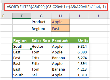
Notice that none of the functions require absolute references, since they only exist in one cell, and spill their results to neighboring cells.

Need more help?

You can always ask an expert in the Excel Tech Community or get support in the Answers community.

See Also

RANDARRAY function

SEQUENCE function

SORT function

SORTBY function

UNIQUE function

#SPILL! errors in Excel

Dynamic arrays and spilled array behavior

Implicit intersection operator: @

Функция ФИЛЬТР позволяет выполнять фильтрацию диапазона данных на основе определенных условий.

Описание функции ФИЛЬТР

Синтаксис

=ФИЛЬТР(массив; включить; [если_пусто])

Аргументы

Замечания

• Функция ФИЛЬТР (FILTER) использует возможности динамических массивов Excel, это означает, что результат вычисления будет автоматически распространяться на смежные ячейки. Также это означает, что нет необходимости фиксировать ячейки абсолютными ссылками в формуле, равно как и использовать автозаполнение;
• Если нужно отфильтровать значение по нескольким условиям, то для логического И используется знак умножения *

  

  На рисунке выше представлен результат фильтрации по продукту Яблоко из региона Восток;

• Если нужно отфильтровать значение по нескольким условиям, то для логического ИЛИ используется знак суммирования +

  

  На рисунке выше диапазон отфильтрован по продукту Яблоко или из региона Восток;

• Если результат вычисления формулы должен заполнить ячейки, которые уже заняты, то будет возвращена ошибка #ПЕРЕНОС!
  

  После очистки ячейки/ ячеек, которые «стоят на пути» вычисления формулы, формула вернет результат.

Пример

Видео работы функции

Дополнительные материалы

Файл из видео.

Microsoft добавила динамические массивы в Excel и новые функции.

Функции динамических массивов: СОРТ, ФИЛЬТР и УНИК

Эта статья является логическим продолжением предыдущего материала про новые динамические массивы (ДМ), появившиеся в Excel в Office 365. Если вы ещё с не ознакомились (кому лень читать — там есть видео), то очень советую сделать это сейчас, чтобы понимать о чём, собственно, идёт речь и как заполучить все эти радости в вашем Excel.

Обновление Office 365, которое подарило Microsoft Excel новый вычислительный движок с поддержкой динамических массивов, также добавило к нашему арсеналу 7 новых функций, заточенных специально для работы с массивами. В этой статье я хотел бы рассказать про три самых важных функции: СОРТ, ФИЛЬТР и УНИК. Остальные играют скорее вспомогательную роль — про них чуть позже.

Для простоты я буду во всех примерах я буду показывать работу этих функций на обычных таблицах, но можно иметь ввиду, что с «умными» таблицами (созданными через Главная — Форматировать как таблицу или сочетанием клавиш Ctrl+T) эти функции тоже отлично работают.

Итак, поехали…

Функция СОРТ (SORT)

Синтаксис:

=СОРТ(массив; [индекс_сортировки]; [порядок_сортировки]; [по_столбцу])

В самом простом варианте требует в качестве аргумента только массив (диапазон) и выдает его уже в отсортированном виде:

По умолчанию сортировка выполняется по возрастанию. Если нужен обратный порядок, то за это отвечает третий аргумент (1 — по возрастанию, -1 — по убыванию):

Если на входе указать диапазон из несколько колонок в данных, то сортировка происходит по первому столбцу. Если нужно сортировать не по первому, то в качестве второго аргумента можно указать номер столбца для сортировки:

Если хочется сортировать по нескольким столбцам сразу, то придётся задать массив номеров столбцов во втором аргументе в фигурных скобках. Одновременно аналогичным образом можно задать третьим аргументом и направление сортировки для каждого столбца.

Например, если мы хотим отсортировать наш список по городам по возрастанию и затем по суммам по убыванию, то это будет выглядеть так:

Последний аргумент используется, если нужно сортировать не строки, а столбцы, т.е. упорядочивать данные по горизонтали, что встречается существенно реже.

Вот так — просто и изящно. Особенно, если вспомнить какую монстрообразную формулу массива требовалось ввести раньше для сортировки всего лишь одного (!) столбца:

Бррр…

Функция ФИЛЬТР (FILTER)

Синтаксис:

=ФИЛЬТР(массив; включить; [если_пусто])

Назначение этой функции — принять в качестве аргумента массив исходных ячеек и отфильтровать его по заданному условию(ям). Какие строки включить в результаты, а какие убрать — определяется вторым аргументом. Он должен представлять из себя массив логических значений ЛОЖЬ (FALSE) и ИСТИНА (TRUE), задающих статус для каждой строки:

Логическую ИСТИНУ и ЛОЖЬ можно, для компактности, заменить на 1 (или любое другое число) и 0 (или пустую ячейку):

А самое интересное, что логические значения могут быть результатом какого-либо выражения, например:

Если чуть подумать, то простор для фантазии тут открывается широкий. Вот вам для затравки несколько вариантов условий, с которыми замечательно будет работать эта функция:

• =ФИЛЬТР(B2:D25; D2:D25>=10000) — отбираем все заказы, где стоимость больше или равна 10 000
• =ФИЛЬТР(B2:D25; ЛЕВСИМВ(B2:B25) = «Б») — фильтрация всех строк, где название товара начинается с «Б» (блуза, брюки, бриджи и т.д.)
• =ФИЛЬТР(B2:D25; (B2:B25 = «Брюки») * (C2:C25 = «Анна»)) — отбор всех сделок Анны, где она продавала брюки
• =ФИЛЬТР(B2:D25; (C2:C25 = «Анна») + (C2:C25 = «Иван»)) — все сделки Анны и Ивана
• =ФИЛЬТР(B2:D25; ЕСЛИОШИБКА(ПОИСК(«Самара»;A2:A25);0)) — фильтрация всех сделок, где в названии города содержится слово Самара (г. Самара, Самара г., город Самара, Самара-городок и т.д.)

Если функция ФИЛЬТР не находит ни одного значения, удовлетворяющего условию, то она выдаёт ошибку #ВЫЧИСЛ! Чтобы вывести вместо неё что-то более осмысленное, можно использовать третий аргумент:

Функция УНИК (UNIQUE)

Синтаксис:

=УНИК(массив; [по_столбцам]; [один_раз])

В самом простом варианте эта функция извлекает из входного массива все имеющиеся там значения, удаляет повторы и выдаёт то, что осталось:

Если в качестве исходного массива выделено несколько столбцов, то проверка на уникальность идёт по всем, т.е. по связке значений из всех ячеек каждой строки:

Очень интересно работает третий аргумент — он заставляет функцию извлечь из исходного массива только те данные, которые встречаются там всего один раз, т.е. не имеют клонов:

Комбинирование функций

Само-собой, никто не запрещает нам «женить» все упомянутые функций между собой — здесь-то и начинается настоящая магия, мощь и синергия.

Разберём, для примера, классическую задачу: предположим, что нам нужно сформировать справочник по городам для выпадающего списка на основе выгрузки из какой-нибудь базы данных. В исходной выгрузке города повторяются в случайном порядке, есть пустые ячейки и дубли. А необходимый нам справочник, содержащий эталонный набор городов, должен быть:

• без повторов
• без пустых ячеек
• отсортирован по возрастанию от А до Я

Делается всё вышеперечисленное одной (!) формулой:

В английской версии эта функция выглядит как:

=SORT(UNIQUE(FILTER(B2:B100000;NOT(ISEMPTY(B2:B100000)))))

Здесь:

• ФИЛЬТР — отбирает только те ячейки, где есть данные (не пусто)
• УНИК — убирает повторы в отобранном функцией ФИЛЬТР списке
• СОРТ — сортирует получившийся справочник по алфавиту

После этого останется только указать получившийся динамический массив как источник для выпадающего списка на вкладке Данные — Проверка данных (Data — Validation), не забыв добавить после адреса первой ячейки массива знак решётки:

Причем, несмотря на приличный размер исходного диапазона (100 тыс. строк!) никакого торможения при пересчёте такой формулы нет абсолютно — новый вычислительный движок Excel справляется «на ура». При этом классические формулы массива на подобных задачах начинали ощутимо подтупливать на таблицах уже с 3-5 тыс. строк, а на 100 тыс. просто загнали бы ваш Excel в кому.

Оглядываясь назад и вспоминая все свои выполненные проекты по автоматизации за последние Х лет, с грустью понимаю сколько дней и даже, наверное, недель можно было бы сэкономить, если бы динамические массивы и такие функции существовали тогда. Даааа….

Ну, лучше поздно, чем никогда, верно? По крайней мере, нашим детям точно будет проще

Ссылки по теме

• Что такое динамические массивы в новом Excel и как они работают
• Как отсортировать список формулой
• Как создать выпдающий список в ячейке листа Excel

Author: Oscar Cronquist Article last updated on January 26, 2023

The FILTER function lets you extract values/rows based on a condition or criteria. It is in the Lookup and reference category and is only available to Excel 365 subscribers.

1. FILTER Function Syntax

FILTER(array, include, [if_empty])

2. FILTER Function Arguments

Argument	Text
array	Required. Cell range or array.
include	Required. An array containing True or False that match the rows and columns of the array argument.
[if_empty]	Optional. The FILTER function returns #CALC! if the result is empty. [if_empty] is a value you define to avoid the #CALC! error.

3. FILTER Function example

The image above shows a regular formula in cell D3:

=FILTER(C3:C7, B3:B7=F2)

The formula above filters the data set in cell range C3:C7 based on the condition specified in cell F2. The output is an array and is returned to cell F4 and cells below as far as needed.

4. Filter values based on a condition

The Filter function filters values in cell range C3:C7 if a value in B3:B7 on the corresponding row equals «France» (Cell F2).

Formula in cell D3:

=FILTER(C3:C7, B3:B7=F2)

There is a formula for you that have an earlier Excel version than Excel 365: VLOOKUP — Return multiple values [vertically]

The FILTER function has three arguments, the second one is an array that evaluates to TRUE or FALSE or their numerical equivalents 1 or 0 (zero).

FILTER(array, include, [if_empty])

B3:B7=F2

The equal sign is a logical operator that evaluates if cell values in B3:B7 are equal to cell value in F2, one by one.

Note, the equal sign is not a case-sensitive. For example, «m» = «M» evaluates to True.

B3:B7=F2

becomes

{«Germany»;»Italy»;»France»;»Italy»;»France»}=»France»

becomes

{«Germany»=»France»;»Italy»=»France»;»France»=»France»;»Italy»=»France»;»France»=»France»}

and returns {FALSE; FALSE; TRUE; FALSE; TRUE}.

The image above shows the array in column A, the values correspond to the values in column B, True is on the same row as France row 5 and 7. False is on all remaining rows.

The FILTER function uses this array containing boolean values (TRUE or False) to determine which values to return from column C. «Apple» and «Lemon» are on the same row as France row 5 and 7. The values are returned to cell F4 and cells below if needed.

The FILTER function may return an array and Microsoft calls this a dynamic array meaning the values are automatically entered to cells below without the need for an array formula.

Back to top

1.1 Why does the FILTER function return a #NAME? error?

First, make sure you correctly spelled the FILTER function. If the FILTER function still returns a #NAME? error you probably use an earlier Excel version and can’t the FILTER function unless you upgrade to Excel 365.

There is a small formula you can use if you don’t have access to the FILTER function, check it out here: VLOOKUP — Return multiple values [vertically]

1.2 Is the FILTER function available for Excel versions 2003, 2007, 2010, 2013, 2016, and 2019?

No, only Excel 365 subscribers have it. However, I made a small formula that works fine, check it out here: VLOOKUP — Return multiple values [vertically]

1.3 The FILTER function returns a #SPILL! error, why?

The FILTER function returns an array of values and tries to automatically use the appropriate cell range needed to show all values. If one or more cells are occupied with other values the FILTER  function returns #SPILL! error.

You have two options, delete or move the values that cause the error or deploy the FILTER function in another cell that has empty cells below.

1.4 Why does the FILTER function return a #CALC! error?

The FILTER function returns a #CALC! error if the output result has no values, make sure you enter the third argument to define a value if dynamic array is empty, to avoid the #CALC! error.

1.5 Can I use the FILTER function with an Excel Table and structured references?

Yes, you can. The FILTER function recalculates the output automatically if you add, edit or delete values in the Excel Table.

Note, the FILTER function does not care if the Excel Table is filtered or not, all matching values will be displayed hidden or not.

1.6 Can the FILTER function handle error values?

No, the FILTER function stops working if there are error values in the second argument. An error in the first argument is passed on to the output array with other regular values.

1.7 Is the FILTER function case sensitive?

No, the FILTER function is not case sensitive if you use the equal sign. Read the next section for how to make the FILTER function case sensitive.

Back to top

5. Filter values based on a condition — case sensitive

The image above shows a formula in cell F4 that extracts values from column C if the corresponding values in column B match the value in cell F2.

=FILTER(C3:C7,EXACT(B3:B7,F2))

There is a formula for you that have an earlier Excel version than Excel 365: Case sensitive lookup and return multiple values

The EXACT function returns True if both arguments are exactly the same considering upper and lower letters as well.

EXACT(text1, text2)

The EXACT function allows you to use a cell range in the first argument and the result is an array that matches the size of the first argument as long as the second argument is a single value.

EXACT(B3:B7,F2)

becomes

EXACT({«france»; «Italy»; «France»; «Italy»; «france»}, «france»)

and returns {TRUE; FALSE; FALSE; FALSE; TRUE}.

FILTER(C3:C7,EXACT(B3:B7,F2))

becomes

FILTER(C3:C7,{TRUE; FALSE; FALSE; FALSE; TRUE})

becomes

FILTER({«Pear»; «Orange»; «Apple»; «Banana»; «Lemon»}, {TRUE; FALSE; FALSE; FALSE; TRUE})

and returns {«Pear»; «Lemon»} in cell range F4:F5.

Back to top

6. Filter values if not equal to

The image above demonstrates the FILTER function in cell F4, it returns all values from column C if the corresponding values in column B are not equal to the value in cell F2.

=FILTER(C3:C7,B3:B7<>F2)

The less than and larger than characters combined means «not equal to».

B3:B7<>F2

becomes

{«Germany»; «Italy»; «France»; «Italy»; «France»}<>»France»

and returns {TRUE; TRUE; FALSE; TRUE; FALSE}.

FILTER(C3:C7,B3:B7<>F2)

becomes

FILTER({«Pear»;»Orange»;»Apple»;»Banana»;»Lemon»}, {TRUE; TRUE; FALSE; TRUE; FALSE})

and returns {«Pear»; «Orange»; «Banana»} in cell range F4:F6.

Back to top

7. Filter values smaller than a condition

The image above shows a formula in cell F4 that extracts values from column B if the corresponding value in column C is less than the number in cell F2.

=FILTER(B3:B7,C3:C7<F2)

The less than character < is a logical operator that checks if a number is smaller than another number. In this demonstration, we will apply this to a cell range C3:C7. The logical expression is:

C3:C7<F2

becomes

{6;2;7;3;2}<5

and returns {FALSE; TRUE; FALSE; TRUE; TRUE}.

FILTER(B3:B7, C3:C7<F2)

becomes

FILTER({«Pear»; «Orange»; «Apple»; «Banana»; «Lemon»}, {FALSE; TRUE; FALSE; TRUE; TRUE})

and returns {«Orange»; «Banana»; «Lemon»}.

Back to top

8. Filter values if larger than the given condition

Formula in cell F4:

=FILTER(B3:B7,C3:C7>F2)

The larger than character > is a logical operator that evaluates to True if a number is larger than another number otherwise False. In this demonstration, we will apply this to a cell range C3:C7. The logical expression is:

C3:C7>F2

becomes

{6;2;7;3;2}>5

and returns {TRUE; FALSE; TRUE; FALSE; FALSE}.

FILTER(B3:B7, C3:C7>F2)

becomes

FILTER({«Pear»;»Orange»;»Apple»;»Banana»;»Lemon»}, {TRUE; FALSE; TRUE; FALSE; FALSE})

and returns {«Pear»; «Apple»}.

Back to top

9. Filter values if cell contains given string

The image above shows a formula in cell F4 that extracts values from column C if the corresponding value in column B contains the given string in cell F2.

Formula in cell F4:

=FILTER(C3:C7,ISNUMBER(SEARCH(F2,B3:B7)))

The formula in cell F4 returns «Pear», «Apple» and «Lemon» because the corresponding values in column B «Germany», «France» and «France» contain string «r».

Step 1 — Identify cells containing string

The SEARCH function has these arguments: SEARCH(find_text,within_text, [start_num])

It returns a number representing the character position of the found string, an error is returned if not found. The SEARCH function does not perform a case sensitive search, use the FIND function for that.

SEARCH(F2,B3:B7))

becomes

SEARCH(«r»,{«Germany»; «Italy»; «France»; «Italy»; «France»}))

and returns {3; #VALUE!; 2; #VALUE!; 2}.

Step 2 — Replace errors

The FILTER function can’t handle errors in the second argument include. FILTER(array, include, [if_empty])

ISNUMBER(SEARCH(F2,B3:B7))

becomes

ISNUMBER({3; #VALUE!; 2; #VALUE!; 2})

and returns {TRUE; FALSE; TRUE; FALSE; TRUE}.

Step 3 — Filter array

FILTER(C3:C7,ISNUMBER(SEARCH(F2,B3:B7)))

becomes

FILTER(C3:C7, {TRUE; FALSE; TRUE; FALSE; TRUE})

becomes

FILTER({«Pear»; «Orange»; «Apple»; «Banana»; «Lemon»}, {TRUE; FALSE; TRUE; FALSE; TRUE})

and returns {«Pear»; «Apple»; «Lemon»}.

Back to top

10. Filter values if cell doesn’t contain the given string

The image above shows a formula in cell F4 that extracts values from column C if the corresponding value in column B does not contain the given string in cell F2.

Formula in cell F4:

=FILTER(C3:C7,ISERROR(SEARCH(F2,B3:B7)))

The formula in cell F4 returns «Orange» and «Banana» because the corresponding values in column B «Italy» and «Italy» do not contain string «r».

Step 1 — Identify cells that contain the string

The SEARCH function has these arguments: SEARCH(find_text,within_text, [start_num])

It returns a number representing the character position of the found string, an error is returned if not found. The SEARCH function does not perform a case sensitive search, use the FIND function for that.

SEARCH(F2,B3:B7))

becomes

SEARCH(«r»,{«Germany»; «Italy»; «France»; «Italy»; «France»}))

and returns {3; #VALUE!; 2; #VALUE!; 2}.

Step 2 — Identify errors

The FILTER function can’t handle errors in the second argument include. FILTER(array, include, [if_empty])

ISERROR(SEARCH(F2,B3:B7))

becomes

ISNUMBER({3; #VALUE!; 2; #VALUE!; 2})

and returns {FALSE; TRUE; FALSE; TRUE; FALSE}.

Step 3 — Filter array

FILTER(C3:C7, ISERROR(SEARCH(F2,B3:B7)))

becomes

FILTER(C3:C7, {FALSE; TRUE; FALSE; TRUE; FALSE})

becomes

FILTER({«Pear»; «Orange»; «Apple»; «Banana»; «Lemon»}, {FALSE; TRUE; FALSE; TRUE; FALSE})

and returns {«Orange»; «Banana»} in cell range F4:F5.

Back to top

11. Filter values that begin with

The formula above in cell F4 extracts values from column C if the corresponding value in column B begins with the given string in cell F2.

Formula in cell F4:

=FILTER(B3:C7,LEFT(B3:B7,LEN(F2))=F2)

The formula in cell F4 returns all rows from cell range B3:C7 that begins with the string specified in cell F2.

Step 1 — Calculate character length of value in cell F2

The LEN function counts the characters in a cell or string.

LEN(F2)

becomes

LEN(«00»)

and returns 2.

Step 2 — Extract characters

The LEFT function returns a specific number of characters from a cell value or string starting from the left. LEFT(text,[num_chars])

LEFT(B3:B7,LEN(F2))

becomes

LEFT(B3:B7,2)

becomes

LEFT({«001»; «024»; «008»; «018»; «004»}, 2)

and returns {«00″;»02″;»00″;»01″;»00»}.

Step 3 — Compare with value in cell F2

The equal sign lets you compare values (not case sensitive), it returns a boolean value True or False.

LEFT(B3:B7,LEN(F2))=F2

becomes

{«00″;»02″;»00″;»01″;»00″}=»00»

and returns

{TRUE; FALSE; TRUE; FALSE; TRUE}.

Step 4 — Filter values

FILTER(B3:C7,LEFT(B3:B7,LEN(F2))=F2)

becomes

FILTER(B3:C7,{TRUE; FALSE; TRUE; FALSE; TRUE})

becomes

FILTER({«001», «Pear»; «024», «Orange»; «008», «Apple»; «018», «Banana»; «004», «Lemon»},{TRUE; FALSE; TRUE; FALSE; TRUE})

and returns

{«001″,»Pear»;»008″,»Apple»;»004″,»Lemon»} in cell range F4:G7.

Back to top

12. Filter values that end with a specific string

The formula above in cell F4 extracts values from column C if the corresponding value in column B ends with the given string in cell F2.

Formula in cell F4:

=FILTER(B3:C7, RIGHT(B3:B7, LEN(F2))=F2)

The formula in cell F4 returns all rows from cell range B3:C7 that end with 8 in column B.

Step 1 — Calculate character length of the value in cell F2

The LEN function counts the characters in a cell or string.

LEN(F2)

becomes

LEN(«8»)

and returns 1.

Step 2 — Extract characters

The RIGHT function returns a specific number of characters from a cell value or string starting from the left. LEFT(text,[num_chars])

LEFT(B3:B7,LEN(F2))

becomes

LEFT(B3:B7,1)

becomes

LEFT({«001»; «024»; «008»; «018»; «004»}, 1)

and returns {«1″;»4″;»8″;»8″;»4»}.

Step 3 — Compare with value in cell F2

The equal sign lets you compare values (not case sensitive), it returns a boolean value True or False.

RIGHT(B3:B7,LEN(F2))=F2

becomes

{«1″;»4″;»8″;»8″;»4″}=»8»

and returns

{FALSE; FALSE; TRUE; TRUE; FALSE}.

Step 4 — Filter values

FILTER(B3:C7,LEFT(B3:B7,LEN(F2))=F2)

becomes

FILTER(B3:C7, {FALSE; FALSE; TRUE; TRUE; FALSE})

becomes

FILTER({«001», «Pear»; «024», «Orange»; «008», «Apple»; «018», «Banana»; «004», «Lemon»}, {FALSE; FALSE; TRUE; TRUE; FALSE})

and returns

{«008», «Apple»; «018», «Banana»} in cell range F4:G5.

Back to top

13. Filter values based on a condition sorted A to Z

Formula in cell F4:

=SORT(FILTER(C3:C9,B3:B9=F2))

The formula in cell F4 extracts values from column B based on a condition specified in cell F2, If the condition matches a value in column C the corresponding value from column B is returned. The array is sorted from A to Z.

Step 1 — Logical expression

The equal sign allows you to compare the value in cell F2 to values in cell range B3:B9. The result is an array containing boolean values True or False.

B3:B9=F2

becomes

{«Germany»; «Italy»; «France»; «Italy»; «France»; «Germany»; «France»}=»France»

and returns

{FALSE; FALSE; TRUE; FALSE; TRUE; FALSE; TRUE}

Step 2 — Filter values

The array containing boolean values determine which values in cell range C3:C9 to filter.

FILTER(C3:C9,B3:B9=F2)

becomes

FILTER(C3:C9,{FALSE; FALSE; TRUE; FALSE; TRUE; FALSE; TRUE})

becomes

FILTER({«Pear»; «Orange»; «Grape»; «Banana»; «Apple»; «Strawberry»; «Lemon»}, {FALSE; FALSE; TRUE; FALSE; TRUE; FALSE; TRUE})

and returns

{«Grape»; «Apple»; «Lemon»}.

Step 3 — Sort values

The SORT function is available for Excel 365 users and has the following arguments: SORT(array,[sort_index],[sort_order],[by_col])

It lets you sort an array from A to Z if you leave the remaining arguments, they are optional anyway.

SORT(FILTER(C3:C9,B3:B9=F2))

becomes

SORT({«Grape»; «Apple»; «Lemon»})

and returns

{«Apple»; «Grape»; «Lemon»}

in cell range F4:F6.

Back to top

14. Filter values based on criteria applied to a column

The formula in cell E7 filters the values in cell range B3:C7 based on two values specified in cell range F2:F3.

If any of the two values match a value in column B the corresponding value from column C is returned as well as the matching value.

Formula in cell E7:

=FILTER(B3:C7, COUNTIF(F2:F3, B3:B7))

The COUNTIF function counts values based on a condition or criteria, here is how it is done. COUNTIF(range, criteria)

COUNTIF(F2:F3, B3:B7)

becomes

COUNTIF({«France»; «Italy»}, {«Germany»; «Italy»; «France»; «Italy»; «France»})

and returns

{0; 1; 1; 1; 1}. 0 (zero) is the equivalent to False and every other value positive or negative evaluates to True.

FILTER(B3:C7, {0; 1; 1; 1; 1})

becomes

FILTER({«Germany», «Pear»; «Italy», «Orange»; «France», «Apple»; «Italy», «Banana»; «France», «Lemon»}, {0; 1; 1; 1; 1})

and returns

{«Italy», «Orange»; «France», «Apple»; «Italy», «Banana»; «France», «Lemon»}.

Back to top

15. Filter values based on one condition per column — AND logic

The formula in cell F10 extracts rows from cell range B3:D7 if two conditions are met, specified in cell F4 and G4. The first condition is compared to column B and the second condition is compared to column C.

A row is extracted if both conditions are met on the same row.

Formula in cell F7:

=FILTER(B3:D7, (B3:B7=F4)*(C3:C7=G4))

The first logical expression is B3:B7=F4.

B3:B7=F4

becomes

{«Germany»;»Italy»;»France»;»Italy»;»France»}=»Italy»

and returns

{FALSE; TRUE; FALSE; TRUE; FALSE}

The second logical expression is {2; 5; 4; 6; 3}=5.

{2; 5; 4; 6; 3}=5

returns

{FALSE; TRUE; FALSE; FALSE; FALSE}

To apply AND logic we must multiply the arrays using the asterisk character. The parentheses allow us to control the calculations, we want to calculate the expressions inside the parentheses before we multiple the arrays.

(B3:B7=F4)*(C3:C7=G4)

becomes

({FALSE; TRUE; FALSE; TRUE; FALSE})*({FALSE; TRUE; FALSE; FALSE; FALSE})

and returns

{0; 1; 0; 0; 0}.

Boolean values are automatically converted to their numerical equivalents when we calculate arithmetic operations.

True * True equals 1

True * False equals 0 (zero)

False * True equals 0 (zero)

False * False equals 0 (zero)

FILTER(B3:D7, (B3:B7=F4)*(C3:C7=G4))

becomes

FILTER(B3:D7, {0; 1; 0; 0; 0})

becomes

FILTER({«Germany», 2, «Pear»; «Italy», 5, «Orange»; «France», 4, «Apple»; «Italy», 6, «Banana»; «France», 5, «Lemon»}, {0; 1; 0; 0; 0})

and returns {«Italy», 5, «Orange»}.

Back to top

16. Filter values based on one condition per column — OR logic

The formula in cell F10 extracts rows from cell range B3:D7 if any of the two conditions are met, specified in cell F4 and G4. The first condition is compared to column B and the second condition is compared to column C.

A row is extracted if any of the conditions are met on the same row.

Formula in cell F7:

=FILTER(B3:D7, (B3:B7=F4)+(C3:C7=G4))

The first logical expression is B3:B7=F4.

B3:B7=F4

becomes

{«Germany»;»Italy»;»France»;»Italy»;»France»}=»Italy»

and returns

{FALSE; TRUE; FALSE; TRUE; FALSE}

The second logical expression is {2; 5; 4; 6; 3}=5.

{2; 5; 4; 6; 5}=5

returns

{FALSE; TRUE; FALSE; FALSE; TRUE}

(B3:B7=F4)+(C3:C7=G4)

becomes

({FALSE; TRUE; FALSE; TRUE; FALSE}) + ({FALSE; TRUE; FALSE; FALSE; TRUE})

and returns

{0; 2; 0; 1; 1}

True + True equals 2 (True)

True + False equals 1 (True)

False + True equals 1 (True)

False + False equals 0 (False)

FILTER(B3:D7, (B3:B7=F4)+(C3:C7=G4))

becomes

FILTER({«Germany», 2, «Pear»; «Italy», 5, «Orange»; «France», 4, «Apple»; «Italy», 6, «Banana»; «France», 5, «Lemon»}, {0; 2; 0; 1; 1})

and returns

{«Italy», 5, «Orange»; «Italy», 6, «Banana»; «France», 5, «Lemon»}.

Back to top

17. #CALC! error returns [if_empty] argument

The FILTER function in cell F4 returns a #CALC! error. The value in cell F2 is not found in any of the cells in B3:B7.

=FILTER(C3:C7,B3:B7=F2)

The FILTER function returns #CALC! error instead of an empty array. The third argument allows you to customize what to return if the FILTER function returns nothing, see below.

=FILTER(C3:C7,B3:B7=F2,»No values»)

Back to top