

When filtering data in Excel you may sometimes need to filter by an entire list of values, rather than by just a single/few specified values. There is a way to do this by using formulas, and it is fairly easy! You can use the FILTER and COUNTIF functions to filter based on a list in Excel.
To filter by a list in Excel, use the COUNTIF function to give an indication of whether or not each row meets your criteria, and then use the FILTER function to filter out the rows that do not meet your criteria.
There is also a way to filter by a list without using formulas, but it takes longer and is more difficult. Simply using formulas is the easiest way to filter by a list in Excel.
To filter by a list of values in Excel, do the following:
- Use the COUNTIF function to check whether or not each row in your source data should be included in your filter results (i.e. Check to see if any of the values in the list to filter by are found within your data to be filtered). Example: =COUNTIF(F2:F10,A3)
- Use the FILTER function to filter the source data, using the column that the COUNTIF function is in as the criteria column. Example: =FILTER(A3:C100,D3:D100=1)
Here are formulas that you can use to filter by a list in Excel:
The COUNTIF and FILTER formulas below must both be used to accomplish the task of filtering by a list of items / criteria. Further below I will teach you how to use these formulas together in your sheet to file by a list.
Filter Where Found in List
- =COUNTIF(F2:F12,A3)
- =FILTER(A3:C17,D3:D17=1)
FILTER Where NOT in List
- =COUNTIF(F2:F12,A3)
- =FILTER(A3:C17,D3:D17<>1)
Filter by list from another sheet
- =COUNTIF(‘Tab 2’!A2:A12,A3)
- =FILTER(A3:C17,D3:D17=1)
- Alternate: =FILTER(‘Tab 1′!A3:C17,’Tab 1’!D3:D17=1)
In this article I will stick to using the FILTER and COUNTIF functions, since this is the faster and more reliable choice for filtering a range by an array in Excel.
This article focuses on filtering by a list in Excel, but check out this article if you want to learn how to filter by a list in Google Sheets.
If you want to learn how to use the FILTER function to perform ordinary filtering tasks, here is an article that will help you learn the FILTER function from the ground up.
But here we will only be filtering by lists/arrays/columns of data.
I have provided multiple examples showing the different ways to set up the formulas depending on how your data is arranged (i.e. depending on which tab your data/formula is on).
Filter rows based on a list in one sheet vs. multiple sheets
To start with, we will put our formula, our unfiltered data, and the list to filter by, all on the same tab so that you can easily see how the formula is set up and how it functions. But further below I will show you how to use multiple tabs while filtering by a list.
In the first examples we will start very simple, and filter a range of data, by a single-column / list, where the list that we are going to filter by does not contain any extra entries that are not present in the source data (data to be filtered).
This is not always how it will be in the real world… but this will make it easy to see what the formula is doing.
In this example, we have a set of data that shows a list of employees within an individual department at a company, as well as their contact information. We also have another list that shows employees within the department who are eligible for a bonus.
We are going to filter the data set that shows employees and their contact information, by the list of eligible employees… so that only the contact information data of eligible employees is displayed in the filter output.
The task: Show employee contact information for employees who are eligible for a bonus
The logic: In column D, use the COUNTIF function to check whether the names in column A are contained in the list to filter by in the range F3:F17. Filter the range A3:C17, where the values in the range D3:D17 are equal to 1.
The formulas: The COUNTIF formula below, is entered in cell D3, and is copied into the cells below it to fill column D. The FILTER formula below is entered in cell H3.
=COUNTIF(F2:F12,A3)
=FILTER(A3:C17,D3:D17=1)
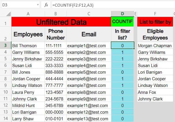
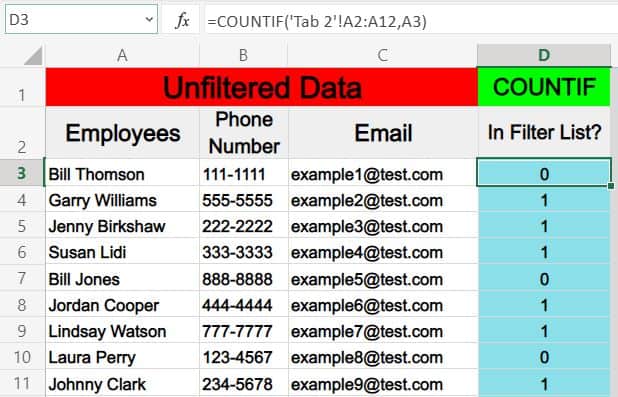
As shown in the example above, column D is being used as a place for the COUNTIF function to provide a simple indication of whether each name in column A is found within the «list to filter by» in column F.
If the name is found in the list the cell will display the number 1, and if it is not found in the list the cell will display the number 0.
This allows you to use column D as the criteria for the filter function, where you can simply tell Excel via the FILTER function to show only the rows where column D is equal to 1 (as shown below).
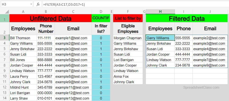
Now the filtered results in columns H through I only show the rows containing names / employees who are on the eligibility list.
Filter based on a list in Excel, where the criteria is NOT found in list
So in this example, let’s say that we want to use the same data / list to filter by as the previous example, but in this case we want to show only the rows where the name is NOT in the eligibility list. In other words we will display a list of employees who are NOT eligible for a bonus.
You might have already recognized that you can do this by changing the filter criteria from «=1» to «=0». This will definitely work, but you might not always be dealing with numbers as a part of your FILTER formula criteria, and so if you ever need to filter rows where NOT equal to a certain string of text, you’ll need to know how to use the «Not equal to» operator / sign in Excel.
The «Not equal to» sign in Excel is expressed like this <>, which is a «less than» symbol followed by a «greater than» symbol. We will use this below to display only rows that are not equal to 1.
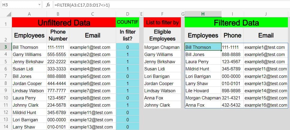
The task: Show employee contact information for employees who are NOT eligible for a bonus
The logic: In column D, use the COUNTIF function to check whether the names in column A are contained in the list to filter by in the range F3:F17. Filter the range A3:C17, where the values in the range D3:D17 are NOT equal to 1.
The formulas: The COUNTIF formula below, is entered in cell D3, and is copied into the cells below it to fill column D. The FILTER formula below is entered in cell H3.
=COUNTIF(F2:F12,A3)
=FILTER(A3:C17,D3:D17<>1)
Filtering by a list when the data is on separate sheets
Now that you know how to filter by a list where all of the data and the formula are held on the same sheet/tab, let’s go over how to filter by a list when using multiple tabs.
There are a variety of arrangements that are possible when using multiple tabs for filtering a range by an array, and so I’ll go over each of them.
In the examples below, both the unfiltered source data (data to be filtered) and the list to filter by are given in the format of multiple column ranges. In other words, the list that we want to filter by is provided with other columns of data beside it this time. This will not change how we setup the formula, but it is important to learn how to identify your column references with data that looks like this.
This type of situation where the list to filter by is attached to other data can be expected in the real world… but it presents another potentially confusing situation with setting up your formula references because of the added columns. i.e. It’s easier to identify the list to filter by when the list is just a single column.
Again, if you are setting up a formula and you find yourself confused, first determine which data needs to be filtered, and which data you are using to filter with/by, then use the COUNTIF with the FILTER function as explained in this lesson.
Source data and formula on the same sheet
Here is an example showing how to set up your formula when the unfiltered source data and filter formula are on the same tab… but where your list that you want to filter by is on a separate tab.
Unfiltered source data & COUNTIF function: Tab 1
FILTER formula: Tab 1
List to filter by: Tab 2
The formulas: The COUNTIF formula below, is entered in cell D3 of Tab 1, and is copied into the cells below it to fill column D. The FILTER formula below is entered in cell F3 of Tab 1.
=COUNTIF(‘Tab 2’!A2:A12,A3)
=FILTER(A3:C17,D3:D17=1)
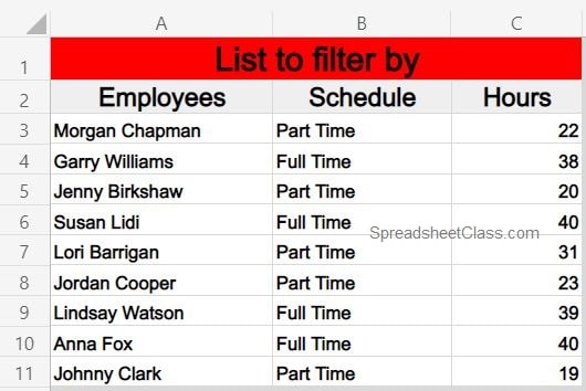
The list that you will use as the criteria in this example is on it’s own tab, as shown above.
Directly below is the «Unfiltered Data». As you can see the COUNTIF function is being used like in the previous examples, to provide a clear indication of whether or not each row in the unfiltered data should appear in the filter results (Whether or not the name in column A is found in the «List to filter by»).

List to filter by and formula on the same sheet
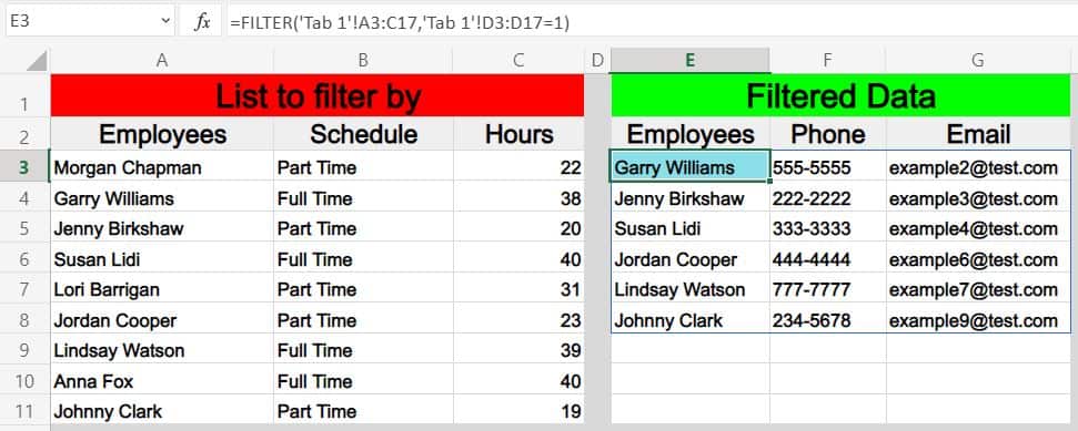
Here is an example showing how to set up your formula when the list that you want to filter by and the formula are on the same tab, but the unfiltered source data is on a separate tab.
Unfiltered source data & COUNTIF function: Tab 1
List to filter by: Tab 2
FILTER formula: Tab 2
The formulas: The COUNTIF formula below, is entered in cell D3 on Tab 1, and is copied into the cells below it to fill column D. The FILTER formula below is entered in cell E3 in Tab 2.
=COUNTIF(‘Tab 2’!A2:A12,A3)
=FILTER(‘Tab 1′!A3:C17,’Tab 1’!D3:D17=1)
Source data, list to filter by, and formula, all on separate sheets
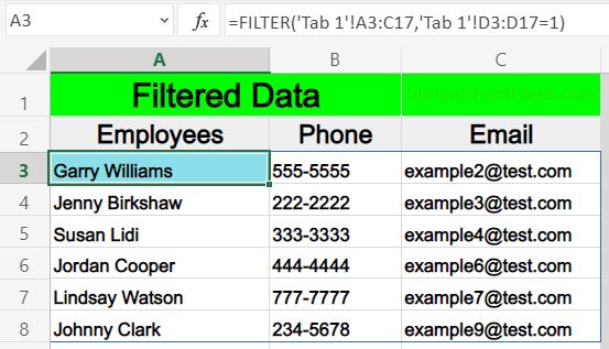
Finally, here is an example showing how to set up your formula when the unfiltered source data (data to be filtered), the list to filter by, and the formula are each on a separate tab.
Unfiltered source data / COUNTIF function: Tab 1
List to filter by: Tab 2
FILTER formula: Tab 3
The formulas: The COUNTIF formula below, is entered in cell D3 in Tab 1, and is copied into the cells below it to fill column D. The FILTER formula below is entered in cell H3 in Tab 3.
=COUNTIF(‘Tab 2’!A2:A12,A3)
=FILTER(‘Tab 1′!A3:C17,’Tab 1’!D3:D17=1)
Pop Quiz: Test your knowledge
Answer the questions below about filtering based on a list, to refine your knowledge! Scroll to the very bottom to find the answers to the quiz.
Question #1
Which of the following formulas has a criteria range of C3:C10?
- =FILTER(A3:C10,D3:D10=1)
- =FILTER(A3:C10,C3:C10=1)
- =FILTER(C3:C10,D3:D10=1)
Question #2
Which of the following formulas has a source range of A3:G?
- =FILTER(C3:C10,G3:G10=1)
- =FILTER(A3:C10,A3:A10=1)
- =FILTER(A3:G10,D3:D10=1)
Question #3
True or False: The COUNTIF function can be used to create a «Criteria column» for the FILTER function.
- True
- False
Answers to the questions above:
Question 1: 2
Question 2: 3
Question 3: 1
Bottom line: Learn 2 ways to filter for a list of multiple items in Excel in this article and video tutorial.
Skill level: Beginner
The following video is from The Filters 101 Course. In this video I explain two ways to apply a filter for a list of multiple items. These techniques use the Filter Drop-down menus in Excel.
Sample Video from The Filters 101 Course
The video above is from The Filters 101 Course. Filters 101 is an online video course with over 40 video lessons like the one above.

Click here to learn more about The Filters 101 Course
Filtering for Multiple Items
A few questions come in this week from Jennifer and Justin on how to apply a filter for a list of multiple items. This can be a time-consuming task if you try to check all the boxes for different items in the filter drop-down menus. Especially if the filter list contains a lot of items.
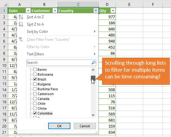
We find ourselves scrolling up and down the list to check each checkbox for all items in our list. There are a few ways to speed up this process. Let’s take a look at two methods that can save us time.
Method #1 – Add current selection to filter
The first method for filtering for a list of items uses an option in the filter drop-down list box called “Add current selection to filter”. As the name suggests, this feature allows us to use the Search box to search for an item, then add the selected items to the current filter criteria.
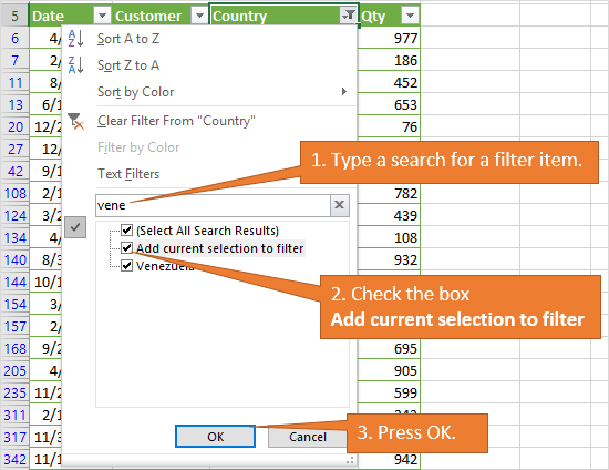
This technique works best when you have 3-5 items to filter for. Here are the steps to use the Add current selection to filter method:
- Use the Search box in the filter drop-down menu to search for the first item.
- Click OK to apply the filter.
- Open the filter drop-down menu again.
- Use the Search box (keyboard shortcut: e) to search for the second item in your filter list.
- Click the “Add current selection to filter” checkbox.
- Click OK. The existing filter criteria will be kept, and the new item will be added to the filter criteria.
- Repeat steps 3 to 6 for each additional item in your filter list.
This process can be time-consuming if you have more than a few items in your filter criteria. See the video above for further explanation on this technique.
It’s also hard to see what items have been filtered for by scrolling through the checkbox list. One tip for this is to hover your mouse over the filter drop-down button. A screentip will appear and display the filter criteria.
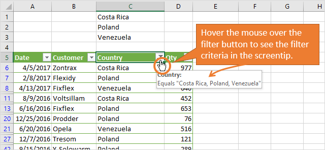
My Filter Mate Add-in will also help with viewing the filter criteria for the filter menus. Check out my post on 7 Keyboard Shortcuts for the Filter Drop-down Menus for more time-saving tips on the filter menus.
Method #2 – Add a Column with a COUNTIF Formula
The second method is a formula based approach that works great for longer lists of filter items.
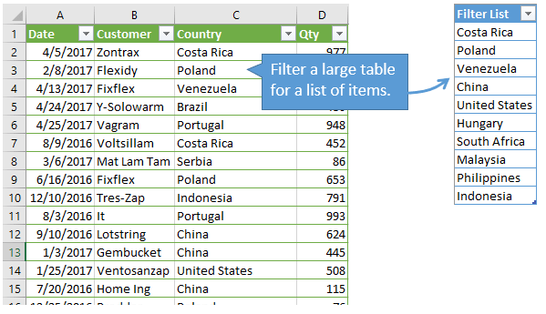
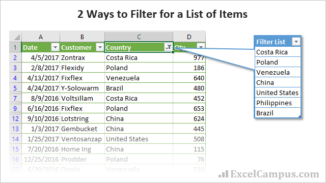
In this example, we want to apply a filter to the data table for a list of countries. This means we only want to see the rows that contain ANY of the countries in the filter list. We can add a column to the data table with a COUNTIF formula.
We use the COUNTIF formula to determine if the country name in the same row in column C exists in the filter list. The filter list is the list of items that we want to filter for. This list can be on the same sheet or a different sheet.
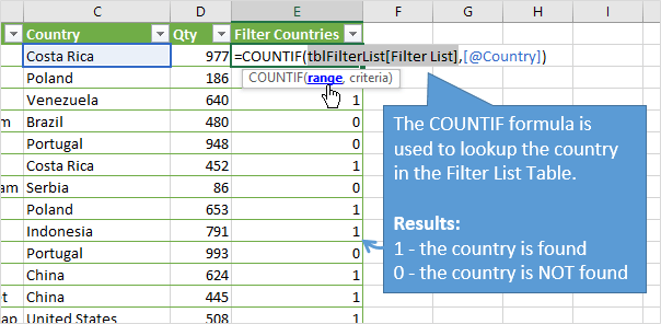
The formula will return:
- 1 if the country exists in the filter list
- 0 if the country does not exist.
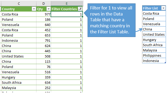
We now have a column of 1’s and 0’s.
Finally, we can apply a filter to the column to filter for 1. This filter will display all the rows where the country in column C matches a country in the filter list.
See my article on using COUNTIF instead of VLOOKUP for more details on the COUNTIF function.
We can also add a “=1” to the end of the formula to return a TRUE or FALSE, instead of 1 or 0.
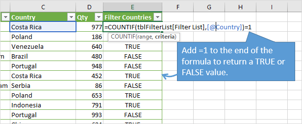
The TRUE or FALSE values will make more sense if you are using the field in a pivot table or slicer, and want to quickly apply a filter for the country list. The TRUE/FALSE is just easier to read and understand versus the 1 or 0. However, the outcome will be the same. See my article on the IF function for more about this TRUE/FALSE boolean logic.
I use Excel Tables for this example. You do NOT have to use Excel Tables for this to work.
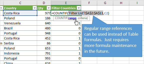
The advantage of using Tables is that we can add new items to the filter list, and we don’t have to modify the formula. Since the formula references the entire column of the Table, there is not maintenance here. We just need to Re-apply the filters (keyboard shortcut: Ctrl+Alt+L) after adding new items to the filter list. This saves time and prevents errors. Win-win! 🙂
Check out my video on A Beginner’s Guide to Excel Tables to learn more about this awesome feature of Excel.
What about Partial Matches that Contain the Filter Criteria?
Arun had a great question in the comments below about filtering for partial matches that contain the filter criteria. We are limited to 2 criteria with the Custom AutoFilter in Excel.
However, we can use this same COUNTIFS technique with wildcard characters to filter for partial matches that contain the criteria. Here is an example of how to modify the formula.
=COUNTIF(tblFilterList[Filter List],"*"&[@Country]&"*")
The asterisk character (*) is a wildcard character that represents any value. To use the wildcard character in the COUNTIF function, we wrap it in quotation marks and use the ampersand symbol to join it to the criteria value.
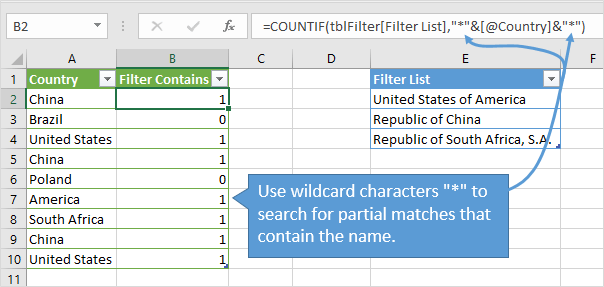
The argument evaluates to *[@Country]*. This means that COUNTIF will look for the country name within the cell, and return a 1 if the name is found within a cell in the range.
The asterisk represents any number of characters before or after the country name. This is the same as a ‘Contains’ type criteria. We can just put the asterisk at the beginning or end if we want to find matching cells that start or end with the lookup value.
We can also use the “?” wildcard character to represent a single character. Here is an example.
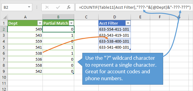
This works great for account codes and phone numbers.
What Techniques Do You Use to Filter Multiple Items?
These are two simple techniques to filter multiple items. With everything in Excel, there are many ways to go about this. Do you use a different technique? If so, please let us know by leaving a comment below. You can also leave a comment with any questions.
I also have a free 3-part video series on Excel Filters. In video #3 of the series, we look at applying filters to multiple columns.
Check Out The Filters 101 Course
The video above is a sample lesson from The Filters 101 Course. This course contains over 40 video lessons just like this one. This is step-by-step training that will help you get the most out of the sort & filter features in Excel, to prepare & analyze your data faster.
Click here to learn more about The Filters 101 Course
Use AutoFilter or built-in comparison operators like «greater than» and “top 10” in Excel to show the data you want and hide the rest. Once you filter data in a range of cells or table, you can either reapply a filter to get up-to-date results, or clear a filter to redisplay all of the data.
Use filters to temporarily hide some of the data in a table, so you can focus on the data you want to see.

Filter a range of data
-
Select any cell within the range.
-
Select Data > Filter.

-
Select the column header arrow
. -
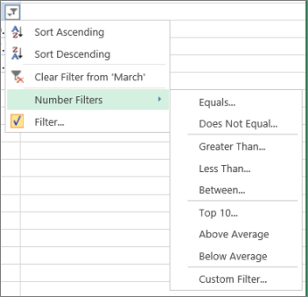
Select Text Filters or Number Filters, and then select a comparison, like Between.
-
Enter the filter criteria and select OK.

 .
.

Filter data in a table
When you put your data in a table, filter controls are automatically added to the table headers.

-
Select the column header arrow
for the column you want to filter. -
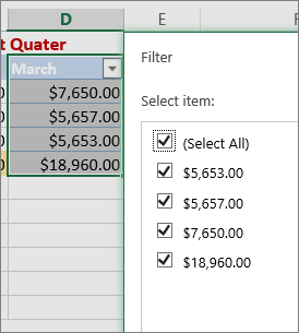
Uncheck (Select All) and select the boxes you want to show.
-
Click OK.
The column header arrow
changes to a Filter icon. Select this icon to change or clear the filter.
 for the column you want to filter.
 Filter icon. Select this icon to change or clear the filter.
Related Topics
Excel Training: Filter data in a table
Guidelines and examples for sorting and filtering data by color
Filter data in a PivotTable
Filter by using advanced criteria
Remove a filter
Filtered data displays only the rows that meet criteria that you specify and hides rows that you do not want displayed. After you filter data, you can copy, find, edit, format, chart, and print the subset of filtered data without rearranging or moving it.
You can also filter by more than one column. Filters are additive, which means that each additional filter is based on the current filter and further reduces the subset of data.
Note: When you use the Find dialog box to search filtered data, only the data that is displayed is searched; data that is not displayed is not searched. To search all the data, clear all filters.
The two types of filters
Using AutoFilter, you can create two types of filters: by a list value or by criteria. Each of these filter types is mutually exclusive for each range of cells or column table. For example, you can filter by a list of numbers, or a criteria, but not by both; you can filter by icon or by a custom filter, but not by both.
Reapplying a filter
To determine if a filter is applied, note the icon in the column heading:
-
A drop-down arrow
means that filtering is enabled but not applied.When you hover over the heading of a column with filtering enabled but not applied, a screen tip displays «(Showing All)».
-
A Filter button
means that a filter is applied.When you hover over the heading of a filtered column, a screen tip displays the filter applied to that column, such as «Equals a red cell color» or «Larger than 150».
When you reapply a filter, different results appear for the following reasons:
-
Data has been added, modified, or deleted to the range of cells or table column.
-
Values returned by a formula have changed and the worksheet has been recalculated.
Do not mix data types
For best results, do not mix data types, such as text and number, or number and date in the same column, because only one type of filter command is available for each column. If there is a mix of data types, the command that is displayed is the data type that occurs the most. For example, if the column contains three values stored as number and four as text, the Text Filters command is displayed .
Filter data in a table
When you put your data in a table, filtering controls are added to the table headers automatically.
-
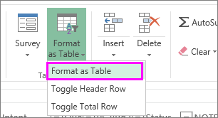
Select the data you want to filter. On the Home tab, click Format as Table, and then pick Format as Table.
-
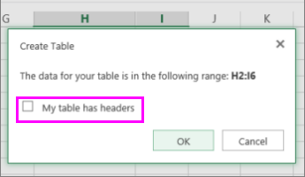
In the Create Table dialog box, you can choose whether your table has headers.
-
Select My table has headers to turn the top row of your data into table headers. The data in this row won’t be filtered.
-
Don’t select the check box if you want Excel for the web to add placeholder headers (that you can rename) above your table data.
-
-
Click OK.
-
To apply a filter, click the arrow in the column header, and pick a filter option.
Filter a range of data
If you don’t want to format your data as a table, you can also apply filters to a range of data.
-
Select the data you want to filter. For best results, the columns should have headings.
-
On the Data tab, choose Filter.
Filtering options for tables or ranges
You can either apply a general Filter option or a custom filter specific to the data type. For example, when filtering numbers, you’ll see Number Filters, for dates you’ll see Date Filters, and for text you’ll see Text Filters. The general filter option lets you select the data you want to see from a list of existing data like this:
Number Filters lets you apply a custom filter:
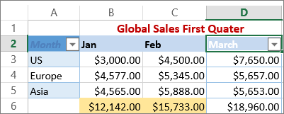
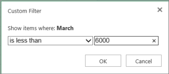
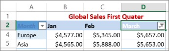
In this example, if you want to see the regions that had sales below $6,000 in March, you can apply a custom filter:
Here’s how:
-
Click the filter arrow next to March > Number Filters > Less Than and enter 6000.
-
Click OK.
Excel for the web applies the filter and shows only the regions with sales below $6000.
You can apply custom Date Filters and Text Filters in a similar manner.
To clear a filter from a column
-
Click the Filter
button next to the column heading, and then click Clear Filter from <«Column Name»>.
To remove all the filters from a table or range
-
Select any cell inside your table or range and, on the Data tab, click the Filter button.
This will remove the filters from all the columns in your table or range and show all your data.
-
Click a cell in the range or table that you want to filter.
-
On the Data tab, click Filter.
-
Click the arrow
in the column that contains the content that you want to filter. -
Under Filter, click Choose One, and then enter your filter criteria.

 in the column that contains the content that you want to filter.
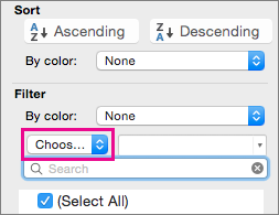
Notes:
-
You can apply filters to only one range of cells on a sheet at a time.
-
When you apply a filter to a column, the only filters available for other columns are the values visible in the currently filtered range.
-
Only the first 10,000 unique entries in a list appear in the filter window.
-
Click a cell in the range or table that you want to filter.
-
On the Data tab, click Filter.
-
Click the arrow
in the column that contains the content that you want to filter. -
Under Filter, click Choose One, and then enter your filter criteria.
-
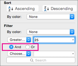
In the box next to the pop-up menu, enter the number that you want to use.
-
Depending on your choice, you may be offered additional criteria to select:
Notes:
-
You can apply filters to only one range of cells on a sheet at a time.
-
When you apply a filter to a column, the only filters available for other columns are the values visible in the currently filtered range.
-
Only the first 10,000 unique entries in a list appear in the filter window.
-
Instead of filtering, you can use conditional formatting to make the top or bottom numbers stand out clearly in your data.
You can quickly filter data based on visual criteria, such as font color, cell color, or icon sets. And you can filter whether you have formatted cells, applied cell styles, or used conditional formatting.
-
In a range of cells or a table column, click a cell that contains the cell color, font color, or icon that you want to filter by.
-
On the Data tab, click Filter .
-
Click the arrow
in the column that contains the content that you want to filter. -
Under Filter, in the By color pop-up menu, select Cell Color, Font Color, or Cell Icon, and then click a color.
 in the column that contains the content that you want to filter.
This option is available only if the column that you want to filter contains a blank cell.
-
Click a cell in the range or table that you want to filter.
-
On the Data toolbar, click Filter.
-
Click the arrow
in the column that contains the content that you want to filter. -
In the (Select All) area, scroll down and select the (Blanks) check box.
Notes:
-
You can apply filters to only one range of cells on a sheet at a time.
-
When you apply a filter to a column, the only filters available for other columns are the values visible in the currently filtered range.
-
Only the first 10,000 unique entries in a list appear in the filter window.
-
-
Click a cell in the range or table that you want to filter.
-
On the Data tab, click Filter .
-
Click the arrow
in the column that contains the content that you want to filter. -
Under Filter, click Choose One, and then in the pop-up menu, do one of the following:
To filter the range for
Click
Rows that contain specific text
Contains or Equals.
Rows that do not contain specific text
Does Not Contain or Does Not Equal.
-
In the box next to the pop-up menu, enter the text that you want to use.
-
Depending on your choice, you may be offered additional criteria to select:
To
Click
Filter the table column or selection so that both criteria must be true
And.
Filter the table column or selection so that either or both criteria can be true
Or.
-
Click a cell in the range or table that you want to filter.
-
On the Data toolbar, click Filter .
-
Click the arrow
in the column that contains the content that you want to filter. -
Under Filter, click Choose One, and then in the pop-up menu, do one of the following:
To filter for
Click
The beginning of a line of text
Begins With.
The end of a line of text
Ends With.
Cells that contain text but do not begin with letters
Does Not Begin With.
Cells that contain text but do not end with letters
Does Not End With.
-
In the box next to the pop-up menu, enter the text that you want to use.
-
Depending on your choice, you may be offered additional criteria to select:
To
Click
Filter the table column or selection so that both criteria must be true
And.
Filter the table column or selection so that either or both criteria can be true
Or.
Wildcard characters can be used to help you build criteria.
-
Click a cell in the range or table that you want to filter.
-
On the Data toolbar, click Filter.
-
Click the arrow
in the column that contains the content that you want to filter. -
Under Filter, click Choose One, and select any option.
-
In the text box, type your criteria and include a wildcard character.
For example, if you wanted your filter to catch both the word «seat» and «seam», type sea?.
-
Do one of the following:
Use
To find
? (question mark)
Any single character
For example, sm?th finds «smith» and «smyth»
* (asterisk)
Any number of characters
For example, *east finds «Northeast» and «Southeast»
~ (tilde)
A question mark or an asterisk
For example, there~? finds «there?»
Do any of the following:
|
To |
Do this |
|---|---|
|
Remove specific filter criteria for a filter |
Click the arrow |
|
Remove all filters that are applied to a range or table |
Select the columns of the range or table that have filters applied, and then on the Data tab, click Filter. |
|
Remove filter arrows from or reapply filter arrows to a range or table |
Select the columns of the range or table that have filters applied, and then on the Data tab, click Filter. |
When you filter data, only the data that meets your criteria appears. The data that doesn’t meet that criteria is hidden. After you filter data, you can copy, find, edit, format, chart, and print the subset of filtered data.
Table with Top 4 Items filter applied
Filters are additive. This means that each additional filter is based on the current filter and further reduces the subset of data. You can make complex filters by filtering on more than one value, more than one format, or more than one criteria. For example, you can filter on all numbers greater than 5 that are also below average. But some filters (top and bottom ten, above and below average) are based on the original range of cells. For example, when you filter the top ten values, you’ll see the top ten values of the whole list, not the top ten values of the subset of the last filter.
In Excel, you can create three kinds of filters: by values, by a format, or by criteria. But each of these filter types is mutually exclusive. For example, you can filter by cell color or by a list of numbers, but not by both. You can filter by icon or by a custom filter, but not by both.
Filters hide extraneous data. In this manner, you can concentrate on just what you want to see. In contrast, when you sort data, the data is rearranged into some order. For more information about sorting, see Sort a list of data.
When you filter, consider the following guidelines:
-
Only the first 10,000 unique entries in a list appear in the filter window.
-
You can filter by more than one column. When you apply a filter to a column, the only filters available for other columns are the values visible in the currently filtered range.
-
You can apply filters to only one range of cells on a sheet at a time.
Note: When you use Find to search filtered data, only the data that is displayed is searched; data that is not displayed is not searched. To search all the data, clear all filters.
Need more help?
You can always ask an expert in the Excel Tech Community or get support in the Answers community.
To make it easy to filter for several different items, you create a list of those items on a worksheet. Then, filter your data based on that list, so you don’t have to check all the items manually each time.
Video: Filter Exact Match List Items
Watch this video to see how to set up an Advanced Filter, and filter for exact matches in the item list.
To get the Microsoft Excel file, so you follow along with the video, go to the Excel Advanced Filter Criteria page on my Contextures site. In the download section, look for the Match Items in List sample workbook
NOTE: There are written steps below the video, for another Filter to Match List Items example.
Your browser can’t show this frame. Here is a link to the page
Two Options for Filtering
Here’s the sample data, and the list of items that we want to filter. The table in column F is named tblFind, and cells F2:F3 are named FindList.

We’ll look at two options for filtering the list:
- Filter rows that have an exact Product match for items in the list
- Filter rows that contain an item in the list, anywhere in the Product field
Advanced Filter
Both options will use an Advanced Filter, so a Criteria range is added to the worksheet.
We’ll be using a formula in the criteria cell, so type a heading that is different from any column header in the data table, or leave the criteria heading blank.

Exact Match For Items in List
For the first filter, we want to find rows with a product that is an exact match for one of the list items.
- In cell C2, enter the following formula. It refers to the named range in the list of items, and the first Product cell in the data table.
=COUNTIF(FindList,C5)
The formula uses the COUNTIF function to check each record, and test for the list items. Rows with an exact match will be returned in the filter.
Run the Advanced Filter
To run the Advanced Filter, and show the results in place, follow these steps:
- Select a cell in the data table
- On the Data tab of the Ribbon, in the Sort & Filter group, click Advanced, to open the Advanced Filter dialog box
- For Action, select Filter the list, in-place
- For List range, select the data table
- For Criteria range, select C1:C2 – the criteria heading and formula cells
- Click OK, to see the results

The 4 rows that have a product that is exactly “Milk” or “Cookies” (case does not matter), are visible, and all other rows are hidden.

Partial Match: Contain Item in List
For the second filter, we want to find rows with a product that contains one of the list items, anywhere in the Product name cell.
- In cell C2, enter the following formula. It refers to the named range in the list of items, and the first Product cell in the data table.
=SUMPRODUCT(COUNTIF(C5,”*”& FindList &”*”))>0
The COUNTIF function checks each Product cell, and tests for the list items. The * wildcards are used before and after the list item, so the text can be found anywhere in the Product cell.
The SUMPRODUCT function sums the number, and if it’s greater than zero, the result is TRUE.
- Tip: See more SUMPRODUCT examples on my Contextures site.
Run the Filter
Next, run the Advanced Filter with the same settings as in the first example, and the 6 rows that contain “Milk” or “Cookies” (upper or lower case does not matter) in the product cell are visible.

Download the Sample File
To get the Excel file for the Exact Match video, go to the Excel Advanced Filter Criteria page on my Contextures site. In the download section, look for the Match Items in List sample workbook
The zipped file is in Excel xlsx format, and does not contain any macros
Related Links
Advanced Filter Basics
Advanced Filter Criteria
Advanced Filter Criteria Slicers
Advanced Filter Macros
Filter to Different Sheet
Filter Unique Items
____________
We can do filter data by some certain criteria for a list or a table in excel. And if the criteria is another list selection in worksheet, how can we filter data from original selected range refer to the new list selection? This article will provide you two methods to filter data based on another list selection by COUNTIF Formula or Advanced Filter Function in excel, you can select one you like to use it in your daily work.
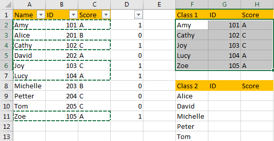
Why we need to learn how to filter data based on another list selection? Actually, we often get a summary (filter range) from others and we just want to get part information by some criteria (criteria range, usually it is another list), see the example below.
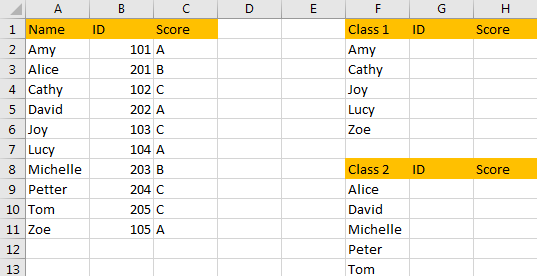
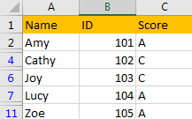
In above table column A, B, C list all students’ Names, IDs and Scores. We want to get ID and Score for class1 and class2 students, we need to filter data from the filter range based on the name list of class1 and class2. Now, you can follow below steps to filter data by different methods.
Table of Contents
- Method 1: Filter Data Based on Another List Selection by Formula
- Method 2: Filter Data Based on Another List Selection by Advanced Filter
- Related Functions
Method 1: Filter Data Based on Another List Selection by Formula
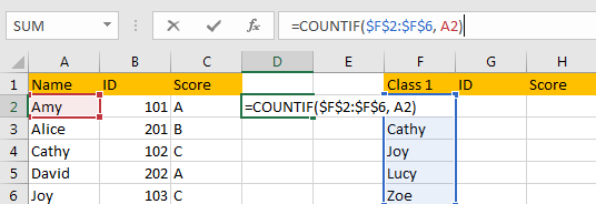
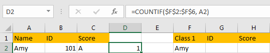
Step 1: First, we need to find out which names included in column A also belong to Class1. We can use COUNTIF function to mark these names. In cell D2, enter the formula =COUNTIF($F$2:$F$6, A2). Then click Enter. Verify that we get return value ‘1’ in D2.
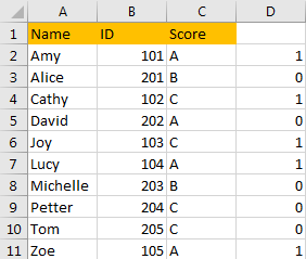
Step 2: Drag the fill handle down to fill all cells. Then we can find that names belong to class1 are marked with number ‘1’.
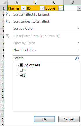
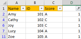
Step 3: Create a filter on column D. Select on column D, click on Data->Filter, then click dropdown list, only check on number ‘1’, then click OK.
Verify that all names belong to class1 are listed properly with ID and Score.
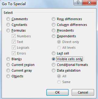
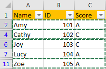
Step 4: Select all filtered data, click F5, on Go To dialog click on Special button, then check on ‘Visible cells only’, then click OK.
Step 5: Copy and paste the selected data to criteria range accordingly.
We can repeat above steps to filter data for class2.
Method 2: Filter Data Based on Another List Selection by Advanced Filter
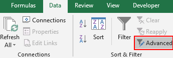
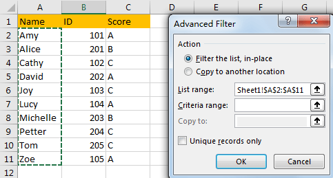
Step 1: Select data you want to do filter, in this case we select A2:C11, select Data->Advanced.
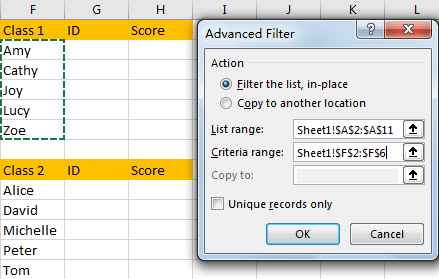
Step 2: On Advanced Filter dialog, check on ‘Filter the list, in-place’, in List range select $A$2:$A$11, in Criteria range, select $F$2:$F$6. Then click OK.
Step 3: After above steps, names are filtered properly.
Step 4: Repeat step#4-5 in method 1 to copy and paste filtered data to criteria range.
- Excel COUNTIF function
The Excel COUNTIF function will count the number of cells in a range that meet a given criteria. This function can be used to count the different kinds of cells with number, date, text values, blank, non-blanks, or containing specific characters.etc.= COUNTIF (range, criteria)…