
This example teaches you how to apply a date filter to only display records that meet certain criteria.
1. Click any single cell inside a data set.
2. On the Data tab, in the Sort & Filter group, click Filter.

Arrows in the column headers appear.

3. Click the arrow next to Date.
4. Click on Select All to clear all the check boxes, click the + sign next to 2015, and click the check box next to January.

5. Click OK.
Result. Excel only displays the sales in 2015, in January.

6. Click the arrow next to Date.
7. Click on Select All to select all the check boxes.
8. Click Date Filters (this option is available because the Date column contains dates) and select Last Month from the list.

Result. Excel only displays the sales of last month.

Note: this date filter and many other date filters depend on today’s date.
To use advanced date filters:
- Select the Data tab, then click the Filter command. A drop-down arrow will appear in the header cell for each column.
- Click the drop-down arrow for the column you want to filter.
- The Filter menu will appear.
- The worksheet will be filtered by the selected date filter.
Contents
- 1 Why can’t I filter dates in Excel?
- 2 How do I filter multiple dates in Excel?
- 3 How do I filter dates by month in Excel?
- 4 How do I filter dates by month and year in Excel?
- 5 How do I filter years from a date in Excel?
- 6 How do I change date format in Excel?
- 7 Can you filter by date range in Excel?
- 8 How do I filter dates in sheets?
- 9 How do I filter pivot by month?
- 10 How do I filter date and time in Excel?
- 11 How do I extract date from datetime in Excel?
- 12 How do I change text filter to date filter in Excel?
- 13 How do I convert date to month and year in Excel?
- 14 How do you autofill dates in Excel without dragging?
- 15 How do I change the date format to MM DD YYYY in Google Sheets?
- 16 What does the filter function do?
- 17 How do I filter a column by date in Google Sheets?
- 18 How do I filter a pivot table by date?
- 19 How do I sort pivot by date?
Why can’t I filter dates in Excel?
Reason 1: Grouping dates in filters is disabled
In Excel, go to File. Click on Options (usually in the left bottom corner of the screen). Go to the Advanced tab in the left pane of the Options window). Scroll down to the workbook settings and set the check at “Group dates in the AutoFilter menu”.
How do I filter multiple dates in Excel?
Filter data between dates
- Generic formula. =FILTER(data,(dates>=A1)*(dates<=A2),»No data»)
- To filter data to include records between two dates, you can use the FILTER function with boolean logic.
- This formula relies on the FILTER function to retrieve data based on a logical test created with a boolean logic expression.
How do I filter dates by month in Excel?
Sorting Dates by Month
- Select the cells in column B (assuming that column B contains the birthdates).
- Press Ctrl+Shift+F.
- Make sure the Number tab is displayed.
- In the Category list, choose Custom.
- In the Type box, enter four lowercase Ms (mmmm) for the format.
- Click on OK.
- Select your entire list.
How do I filter dates by month and year in Excel?
To insert the Auto Filter, select the cell A1 and press the key Ctrl+Shift+L. And filter the data according to the month and year. This is the way we can put the filter by the date field in Microsoft Excel.
How do I filter years from a date in Excel?
To extract the year from a cell containing a date, type =YEAR(CELL) , replacing CELL with a cell reference. For instance, =YEAR(A2) will take the date value from cell A2 and extract the year from it.
How do I change date format in Excel?
Follow these steps:
- Select the cells you want to format.
- Press Control+1 or Command+1.
- In the Format Cells box, click the Number tab.
- In the Category list, click Date.
- Under Type, pick a date format.
Can you filter by date range in Excel?
Filter With Date Checkboxes
If you want to filter for a date range, move the field to the Row or Column area instead.Click the drop down arrow on date field. To show the check boxes, add a check mark to “Select Multiple Items” In the list of dates, add check marks to show dates, or remove check marks to hide dates.
How do I filter dates in sheets?
Below are the steps to sort by date:
- Select the data to be sorted.
- Click the Data option in the menu.
- Click on ‘Sort range’ option.
- In the ‘Sort range’ dialog box: Select the option Data has header row (in case your data doesn’t have a header row, leave this unchecked)
- Click on the Sort button.
How do I filter pivot by month?
Grouping by Months in a Pivot Table
- Select any cell in the Date column in the Pivot Table.
- Go to Pivot Table Tools –> Analyze –> Group –> Group Selection.
- In the Grouping dialogue box, select Months as well as Years. You can select more than one option by simply clicking on it.
- Click OK.
How do I filter date and time in Excel?
- Suppose your data is in range A1:H15 (headings are in A1:H1)
- In cell K1, type Condition.
- In cell K2, enter this formula =MOD(G2,1)<0.5.
- Click on cell A1 and go to Data > Filter > Filter the List in Place.
- In the List range, select A1:H15.
- In the Criteria range, select K1:K2.
- Click on OK.
Extract date from a date and time
- Generic formula. =INT(date)
- To extract the date part of a date that contains time (i.e. a datetime), you can use the INT function.
- Excel handles dates and time using a scheme in which dates are serial numbers and times are fractional values.
- Extract time from a date and time.
How do I change text filter to date filter in Excel?
Click the drop-down arrow for the column you want to filter. In our example, we will filter column D to view only a certain range of dates. The Filter menu will appear. Hover the mouse over Date Filters, then select the desired date filter from the drop-down menu.
How do I convert date to month and year in Excel?
Below are the steps to change the date format and only get month and year using the TEXT function:
- Click on a blank cell where you want the new date format to be displayed (B2)
- Type the formula: =TEXT(A2,”m/yy”)
- Press the Return key.
- This should display the original date in our required format.
How do you autofill dates in Excel without dragging?
The regular way of doing this is: Enter 1 in cell A1. Enter 2 in cell A2. Select both the cells and drag it down using the fill handle.
Quickly Fill Numbers in Cells without Dragging
- Enter 1 in cell A1.
- Go to Home –> Editing –> Fill –> Series.
- In the Series dialogue box, make the following selections:
- Click OK.
How do I change the date format to MM DD YYYY in Google Sheets?
To do this, open your spreadsheet in Google Sheets and press File > Spreadsheet Settings. From the “Locale” drop-down menu, select an alternative location. For instance, setting the locale to “United Kingdom” will switch your spreadsheet to the “DD/MM/YYYY” format and set the default currency to GBP, and so on.
What does the filter function do?
The FILTER function filters an array based on a Boolean (True/False) array. Notes: An array can be thought of as a row of values, a column of values, or a combination of rows and columns of values.The FILTER function will return an array, which will spill if it’s the final result of a formula.
How do I filter a column by date in Google Sheets?
The easiest way to sort a column by date in Google Sheets is to do the following:
- Open the Spreadsheet in Google Sheets.
- Select the Headers of the column(s) you want to sort by date (make sure the column data type is Date)
- Click Data > Create a Filter Option.
- Click on the filter icon.
How do I filter a pivot table by date?
- Navigate to a PivotTable or PivotChart in the same workbook.
- Add a column from the Date table to the Column Labels or Row Labels area of the Power Pivot field list.
- Click the down arrow next to Column Labels or Row Labels in the PivotTable.
- Point to Date Filters, and then select a filter from the list.
How do I sort pivot by date?
In the Pivot Table properties, Under the sort tab: Select the column which u need to sort,Enable the expression option and put the date field. It will work. Then select Column A -In the Expression option, put Start date and select asc or desc based on your requirement.
Use AutoFilter or built-in comparison operators like «greater than» and “top 10” in Excel to show the data you want and hide the rest. Once you filter data in a range of cells or table, you can either reapply a filter to get up-to-date results, or clear a filter to redisplay all of the data.
Use filters to temporarily hide some of the data in a table, so you can focus on the data you want to see.

Filter a range of data
-
Select any cell within the range.
-
Select Data > Filter.

-
Select the column header arrow
. -
Select Text Filters or Number Filters, and then select a comparison, like Between.
-
Enter the filter criteria and select OK.

 .
.

Filter data in a table
When you put your data in a table, filter controls are automatically added to the table headers.

-
Select the column header arrow
for the column you want to filter. -
Uncheck (Select All) and select the boxes you want to show.
-
Click OK.
The column header arrow
changes to a Filter icon. Select this icon to change or clear the filter.
 for the column you want to filter.
 Filter icon. Select this icon to change or clear the filter.
Related Topics
Excel Training: Filter data in a table
Guidelines and examples for sorting and filtering data by color
Filter data in a PivotTable
Filter by using advanced criteria
Remove a filter
Filtered data displays only the rows that meet criteria that you specify and hides rows that you do not want displayed. After you filter data, you can copy, find, edit, format, chart, and print the subset of filtered data without rearranging or moving it.
You can also filter by more than one column. Filters are additive, which means that each additional filter is based on the current filter and further reduces the subset of data.
Note: When you use the Find dialog box to search filtered data, only the data that is displayed is searched; data that is not displayed is not searched. To search all the data, clear all filters.
The two types of filters
Using AutoFilter, you can create two types of filters: by a list value or by criteria. Each of these filter types is mutually exclusive for each range of cells or column table. For example, you can filter by a list of numbers, or a criteria, but not by both; you can filter by icon or by a custom filter, but not by both.
Reapplying a filter
To determine if a filter is applied, note the icon in the column heading:
-
A drop-down arrow
means that filtering is enabled but not applied.When you hover over the heading of a column with filtering enabled but not applied, a screen tip displays «(Showing All)».
-
A Filter button
means that a filter is applied.When you hover over the heading of a filtered column, a screen tip displays the filter applied to that column, such as «Equals a red cell color» or «Larger than 150».
When you reapply a filter, different results appear for the following reasons:
-
Data has been added, modified, or deleted to the range of cells or table column.
-
Values returned by a formula have changed and the worksheet has been recalculated.
Do not mix data types
For best results, do not mix data types, such as text and number, or number and date in the same column, because only one type of filter command is available for each column. If there is a mix of data types, the command that is displayed is the data type that occurs the most. For example, if the column contains three values stored as number and four as text, the Text Filters command is displayed .
Filter data in a table
When you put your data in a table, filtering controls are added to the table headers automatically.
-
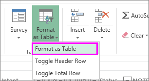
Select the data you want to filter. On the Home tab, click Format as Table, and then pick Format as Table.
-
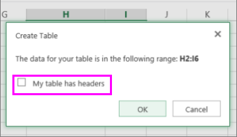
In the Create Table dialog box, you can choose whether your table has headers.
-
Select My table has headers to turn the top row of your data into table headers. The data in this row won’t be filtered.
-
Don’t select the check box if you want Excel for the web to add placeholder headers (that you can rename) above your table data.
-
-
Click OK.
-
To apply a filter, click the arrow in the column header, and pick a filter option.
Filter a range of data
If you don’t want to format your data as a table, you can also apply filters to a range of data.
-
Select the data you want to filter. For best results, the columns should have headings.
-
On the Data tab, choose Filter.
Filtering options for tables or ranges
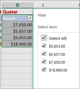
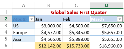
You can either apply a general Filter option or a custom filter specific to the data type. For example, when filtering numbers, you’ll see Number Filters, for dates you’ll see Date Filters, and for text you’ll see Text Filters. The general filter option lets you select the data you want to see from a list of existing data like this:
Number Filters lets you apply a custom filter:
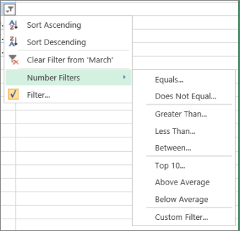
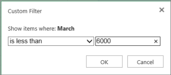
In this example, if you want to see the regions that had sales below $6,000 in March, you can apply a custom filter:
Here’s how:
-
Click the filter arrow next to March > Number Filters > Less Than and enter 6000.
-
Click OK.
Excel for the web applies the filter and shows only the regions with sales below $6000.
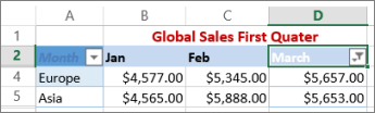
You can apply custom Date Filters and Text Filters in a similar manner.
To clear a filter from a column
-
Click the Filter
button next to the column heading, and then click Clear Filter from <«Column Name»>.
To remove all the filters from a table or range
-
Select any cell inside your table or range and, on the Data tab, click the Filter button.
This will remove the filters from all the columns in your table or range and show all your data.
-
Click a cell in the range or table that you want to filter.
-
On the Data tab, click Filter.
-
Click the arrow
in the column that contains the content that you want to filter. -
Under Filter, click Choose One, and then enter your filter criteria.

 in the column that contains the content that you want to filter.
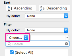
Notes:
-
You can apply filters to only one range of cells on a sheet at a time.
-
When you apply a filter to a column, the only filters available for other columns are the values visible in the currently filtered range.
-
Only the first 10,000 unique entries in a list appear in the filter window.
-
Click a cell in the range or table that you want to filter.
-
On the Data tab, click Filter.
-
Click the arrow
in the column that contains the content that you want to filter. -
Under Filter, click Choose One, and then enter your filter criteria.
-
In the box next to the pop-up menu, enter the number that you want to use.
-
Depending on your choice, you may be offered additional criteria to select:
Notes:
-
You can apply filters to only one range of cells on a sheet at a time.
-
When you apply a filter to a column, the only filters available for other columns are the values visible in the currently filtered range.
-
Only the first 10,000 unique entries in a list appear in the filter window.
-
Instead of filtering, you can use conditional formatting to make the top or bottom numbers stand out clearly in your data.
You can quickly filter data based on visual criteria, such as font color, cell color, or icon sets. And you can filter whether you have formatted cells, applied cell styles, or used conditional formatting.
-
In a range of cells or a table column, click a cell that contains the cell color, font color, or icon that you want to filter by.
-
On the Data tab, click Filter .
-
Click the arrow
in the column that contains the content that you want to filter. -
Under Filter, in the By color pop-up menu, select Cell Color, Font Color, or Cell Icon, and then click a color.
 in the column that contains the content that you want to filter.
This option is available only if the column that you want to filter contains a blank cell.
-
Click a cell in the range or table that you want to filter.
-
On the Data toolbar, click Filter.
-
Click the arrow
in the column that contains the content that you want to filter. -
In the (Select All) area, scroll down and select the (Blanks) check box.
Notes:
-
You can apply filters to only one range of cells on a sheet at a time.
-
When you apply a filter to a column, the only filters available for other columns are the values visible in the currently filtered range.
-
Only the first 10,000 unique entries in a list appear in the filter window.
-
-
Click a cell in the range or table that you want to filter.
-
On the Data tab, click Filter .
-
Click the arrow
in the column that contains the content that you want to filter. -
Under Filter, click Choose One, and then in the pop-up menu, do one of the following:
To filter the range for
Click
Rows that contain specific text
Contains or Equals.
Rows that do not contain specific text
Does Not Contain or Does Not Equal.
-
In the box next to the pop-up menu, enter the text that you want to use.
-
Depending on your choice, you may be offered additional criteria to select:
To
Click
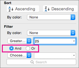
Filter the table column or selection so that both criteria must be true
And.
Filter the table column or selection so that either or both criteria can be true
Or.
-
Click a cell in the range or table that you want to filter.
-
On the Data toolbar, click Filter .
-
Click the arrow
in the column that contains the content that you want to filter. -
Under Filter, click Choose One, and then in the pop-up menu, do one of the following:
To filter for
Click
The beginning of a line of text
Begins With.
The end of a line of text
Ends With.
Cells that contain text but do not begin with letters
Does Not Begin With.
Cells that contain text but do not end with letters
Does Not End With.
-
In the box next to the pop-up menu, enter the text that you want to use.
-
Depending on your choice, you may be offered additional criteria to select:
To
Click
Filter the table column or selection so that both criteria must be true
And.
Filter the table column or selection so that either or both criteria can be true
Or.
Wildcard characters can be used to help you build criteria.
-
Click a cell in the range or table that you want to filter.
-
On the Data toolbar, click Filter.
-
Click the arrow
in the column that contains the content that you want to filter. -
Under Filter, click Choose One, and select any option.
-
In the text box, type your criteria and include a wildcard character.
For example, if you wanted your filter to catch both the word «seat» and «seam», type sea?.
-
Do one of the following:
Use
To find
? (question mark)
Any single character
For example, sm?th finds «smith» and «smyth»
* (asterisk)
Any number of characters
For example, *east finds «Northeast» and «Southeast»
~ (tilde)
A question mark or an asterisk
For example, there~? finds «there?»
Do any of the following:
|
To |
Do this |
|---|---|
|
Remove specific filter criteria for a filter |
Click the arrow |
|
Remove all filters that are applied to a range or table |
Select the columns of the range or table that have filters applied, and then on the Data tab, click Filter. |
|
Remove filter arrows from or reapply filter arrows to a range or table |
Select the columns of the range or table that have filters applied, and then on the Data tab, click Filter. |
When you filter data, only the data that meets your criteria appears. The data that doesn’t meet that criteria is hidden. After you filter data, you can copy, find, edit, format, chart, and print the subset of filtered data.
Table with Top 4 Items filter applied
Filters are additive. This means that each additional filter is based on the current filter and further reduces the subset of data. You can make complex filters by filtering on more than one value, more than one format, or more than one criteria. For example, you can filter on all numbers greater than 5 that are also below average. But some filters (top and bottom ten, above and below average) are based on the original range of cells. For example, when you filter the top ten values, you’ll see the top ten values of the whole list, not the top ten values of the subset of the last filter.
In Excel, you can create three kinds of filters: by values, by a format, or by criteria. But each of these filter types is mutually exclusive. For example, you can filter by cell color or by a list of numbers, but not by both. You can filter by icon or by a custom filter, but not by both.
Filters hide extraneous data. In this manner, you can concentrate on just what you want to see. In contrast, when you sort data, the data is rearranged into some order. For more information about sorting, see Sort a list of data.
When you filter, consider the following guidelines:
-
Only the first 10,000 unique entries in a list appear in the filter window.
-
You can filter by more than one column. When you apply a filter to a column, the only filters available for other columns are the values visible in the currently filtered range.
-
You can apply filters to only one range of cells on a sheet at a time.
Note: When you use Find to search filtered data, only the data that is displayed is searched; data that is not displayed is not searched. To search all the data, clear all filters.
Need more help?
You can always ask an expert in the Excel Tech Community or get support in the Answers community.
На чтение 7 мин. Просмотров 6.8k.
Итог: узнаете, как отфильтровать сводную таблицу, сводную диаграмму или установить срез для самой последней даты или периода в наборе данных.
Уровень мастерства: Средний

Pip имеет набор отчетов на основе сводных таблиц, которые она часто обновляет (ежедневно, еженедельно, ежемесячно). Она хочет автоматически фильтровать отчеты по самой последней дате в столбце в наборе данных. Этот фильтр выберет элемент в слайсере, чтобы отфильтровать сводные таблицы и диаграммы.
Как и все в Excel, есть несколько способов решить эту
проблему. Мы можем использовать макрос или добавить вычисляемый столбец в набор
данных …
Содержание
- Настройка: данные конвейера продаж CRM
- Решение № 1: Макрос VBA для фильтрации сводной
таблицы по определенной дате или периоду - Решение № 2. Добавление вычисляемого столбца в
набор данных - Два способа автоматизации фильтрации сводных
таблиц
Настройка: данные конвейера продаж CRM
В этом примере мы собираемся использовать данные о продажах. Таблица данных содержит еженедельные снимки или экспорт данных из системы CRM (Salesforces.com, Dynamics CRM, HubSpot и т.д.).
Для обновления данных мы
экспортируем конвейерный отчет каждую неделю и вставляем данные в конец
существующей таблицы. Есть и другие способы автоматизации этого процесса, но мы
не будем вдаваться в подробности.

В наборе данных есть
столбец «Дата отчета», в котором содержится дата запуска отчета для каждой строки.
Вы можете видеть на изображении, что есть 4 набора данных, добавленных
(сложенных) вместе, чтобы создать одну большую таблицу.
Сводная таблица показывает
сводку доходов по этапам конвейера, а поле «Дата отчета» находится в области
«Фильтры». Это позволяет нам фильтровать по любой дате отчета, чтобы увидеть
сводную информацию о конвейере за эту неделю.

Когда новые данные
добавляются в таблицу данных, мы хотим автоматически фильтровать все связанные
сводные таблицы, диаграммы и срезы на последнюю дату отчета.
Решение № 1: Макрос VBA для фильтрации сводной
таблицы по определенной дате или периоду
Мы можем использовать
простой макрос, чтобы установить фильтр в сводной таблице для самой последней
даты в таблице исходных данных. Фильтрация поля «Дата отчета» в сводной таблице
также выберет отфильтрованный элемент в срезе и отфильтрует все связанные
сводные диаграммы.
Приведенный ниже макрос
может выглядеть как много кода, но на самом деле он очень прост. Чтобы его
использовать, вам просто нужно будет указать все переменные для имени рабочего
листа, имени сводной таблицы, имени сводного поля (Дата отчета) и критериев
фильтрации (последняя дата). Эти переменные будут представлять имена объектов в
вашей собственной книге.
Sub Filter_PivotField()
' Описание: фильтрация сводной таблицы или среза по определенной дате или периоду.

Dim sSheetName As String
Dim sPivotName As String
Dim sFieldName As String
Dim sFilterCrit As String
Dim pi As PivotItem

    ' Установите переменные
    sSheetName = "Pivot"
    sPivotName = "PivotTable1"
    sFieldName = "Report Date"
    'sFilterCrit = "5/2/2016"
    sFilterCrit = ThisWorkbook.Worksheets("Data").Range("G2").Value

    With ThisWorkbook.Worksheets(sSheetName).PivotTables(sPivotName).PivotFields(sFieldName)
        ' Очистить все фильтры основного поля
        .ClearAllFilters

        ' Проходить по элементам сводки поля сводки
        ' Скрыть или отфильтровать элементы, которые не соответствуют критериям
        For Each pi In .PivotItems
            If pi.Name <> sFilterCrit Then
                pi.Visible = False
            End If
        Next pi

    End With

End Sub
Макрос в настоящее время
настроен на использование значения из ячейки G2 в Таблице данных для критериев
фильтра (самая поздняя дата). Ячейка G2 содержит формулу, которая возвращает
самую последнюю дату из столбца с помощью функции MAX

Конечно, это можно
изменить, чтобы вычислить самую последнюю дату в коде макроса. Хотя приятно
видеть это на листе.
Как работает макрос?
Макрос сначала очищает все
фильтры для поля сводки фильтра отчетов с помощью метода ClearAllFilters.
Затем он использует цикл
For Next для циклического прохождения всех элементов сводки в поле сводки,
чтобы применить фильтр. Каждый уникальный элемент в поле является основным
элементом. Макрос проверяет, не соответствует ли имя элемента сводки (<>)
критериям. Если нет, то он скрывает элемент или фильтрует его. В результате мы
видим только критерии фильтра.
У меня есть статья, которая объясняет For Next Loops более подробно.

Как насчет фильтрации двух сводных таблиц за
разные периоды времени?
Вот еще один пример с
настройкой переменных в качестве параметров макроса. Это позволяет нам вызывать
макрос из другого макроса.
Sub Filter_PivotField_Args( _
    sSheetName As String, _
    sPivotName As String, _
    sFieldName As String, _
    sFilterCrit As String)
' Фильтрация сводной таблицы или среза по определенной дате или периоду
Dim pi As PivotItem

    With ThisWorkbook.Worksheets(sSheetName).PivotTables(sPivotName).PivotFields(sFieldName)
        ' Очистить все фильтры основного поля
        .ClearAllFilters

        ' Проходить по элементам сводки поля сводки
        ' Скрыть или отфильтровать элементы, которые не соответствуют критериям
        For Each pi In .PivotItems
            If pi.Name <> sFilterCrit Then
                pi.Visible = False
            End If
        Next pi
    End With

End Sub
Sub Filter_Multiple_Pivots()
' Вызвать макрос Filter Pivot для нескольких пивотов
Dim sFilter1 As String
Dim sFilter2 As String

    ' Установите критерии фильтра
    sFilter1 = ThisWorkbook.Worksheets("Data").Range("G2").Value
    sFilter2 = ThisWorkbook.Worksheets("Data").Range("G3").Value

    ' Вызовите макрос сводных фильтров, чтобы отфильтровать оба сводных
    Call Filter_PivotField_Args("2 Pivots", "PivotTable1", "Report Date", sFilter1)
    Call Filter_PivotField_Args("2 Pivots", "PivotTable2", "Report Date", sFilter2)

End Sub
В этом примере у нас есть лист с двумя сводными таблицами для сравнения неделя за неделей. Таким образом, нам нужно отфильтровать одну сводную таблицу для самой последней даты и одну для даты предыдущей недели.
Макрос Filter_Multiple_Pivots вызывает макрос Filter_PivotField_Args дважды. Обратите внимание, что имя сводной таблицы и значения критериев фильтрации различны для каждого вызова. Это простой способ многократно использовать макрос сводного поля фильтра без необходимости повторения большого количества кода.
Ознакомьтесь с моей бесплатной серией видео о том, как начать работу с макросами и VBA, чтобы узнать больше о написании макросов.
Решение № 2. Добавление вычисляемого столбца в
набор данных
Если вы не можете использовать макросы, вы можете решить эту проблему с помощью вычисляемого столбца. Это решение НЕ так гибко, как макрос. Оно НЕ очень хорошо работает, если вы хотите иметь срезы, где пользователь может выбирать другие даты отчета.
Мы можем добавить столбец
к исходным данным, чтобы проверить, совпадает ли дата отчета в каждой строке с
самой последней датой. Мы назовем этот столбец «Current Wk».

Если это так, то формула
вернет ИСТИНА, если нет — ЛОЖЬ.
Это очень простая формула.
Мы могли бы использовать функцию If, но в этом нет необходимости. Знак
равенства оценивает совпадение и возвращает значение ИСТИНА или ЛОЖЬ.
Ознакомьтесь с моей статьей If в
формулах Excel для объяснения этого.
Теперь мы можем добавить
этот новый столбец в область «Фильтры» сводной таблицы и отфильтровать его для
ИСТИНА. Это означает, что каждый раз, когда исходные данные обновляются новыми
данными, формулы пересчитывают новые строки текущей недели. Обновление сводной
таблицы автоматически применит фильтр для строк текущей недели и отобразит их в
сводной таблице.

Недостатком здесь является
то, что пользователь не может использовать слайсер для фильтрации других дат.
Технически они могут, но нам придется повторно применить фильтр Current Wk при
следующем обновлении данных. Мы могли бы использовать макрос для автоматизации
этого, но тогда мы действительно вернулись к решению № 1.
Хотя он не такой
динамичный, как решение № 1, рассчитанный столбец может быть всем необходимым
для отображения данных за последний период в статическом отчете.
Два способа автоматизации фильтрации сводных
таблиц
Фильтрация сводных таблиц
по самой последней дате или периоду — это, безусловно, хороший процесс для
автоматизации, если вы часто выполняете эту задачу. Это может сэкономить нам
много времени и предотвратить ошибки, которые обычно возникают при этих скучных
повторяющихся задачах. 🙂
Пожалуйста, оставьте
комментарий ниже с любыми вопросами или предложениями. Спасибо!
Often you may want to filter dates by month in Excel.
Fortunately this is easy to do using the Filter function.
The following step-by-step example shows how to use this function to filter dates by month in Excel.
Step 1: Create the Data
First, let’s create a dataset that shows the total sales made by some company on various days:

Step 2: Add a Filter
Next, highlight the cells in the range A1:B13 and then click the Data tab along the top ribbon and click the Filter button:

A dropdown filter will automatically be added to the first row of column A and column B.
Step 3: Filter Dates by Month
Next, we’ll filter the data to only show the rows where the month contains February.
Click the dropdown arrow next to Date, then uncheck all of the boxes except the one next to February and then click OK:

The data will automatically be filtered to only show the rows where the date is in February:

Note that if you have multiple years and you’d like to filter the data to only show the dates in February (while ignoring year), you can click the dropdown arrow next to Date, then Date Filters, then All Dates in the Period, then February:

The data will automatically be filtered to only show the rows where the date is in February, regardless of the year.
Additional Resources
The following tutorials explain how to perform other common operations in Excel:
How to Group Data by Month in Excel
How to AutoFill Dates in Excel
How to Calculate the Difference Between Two Dates in Excel