
Fill data automatically in worksheet cells
Use the Auto Fill feature to fill cells with data that follows a pattern or are based on data in other cells.

Find more videos on Mike Girvin’s YouTube channel, excelisfun.
-
Select one or more cells you want to use as a basis for filling additional cells.
For a series like 1, 2, 3, 4, 5…, type 1 and 2 in the first two cells. For the series 2, 4, 6, 8…, type 2 and 4.
For the series 2, 2, 2, 2…, type 2 in first cell only.
-
Drag the fill handle
 .
. -
If needed, click Auto Fill Options
and choose the option you want.
 .
. and choose the option you want.
Need more help?
You can always ask an expert in the Excel Tech Community or get support in the Answers community.
Need more help?
Want more options?
Explore subscription benefits, browse training courses, learn how to secure your device, and more.
Communities help you ask and answer questions, give feedback, and hear from experts with rich knowledge.
In Excel, there are many ways to quickly and efficiently fill cells with data. Everyone knows that laziness – is the engine of progress. Know about this and the developers.
To fill in the data you have to spend most of the time on boring and routine work. For example, filling in the time sheet or the invoice, etc.
Let`s consider the techniques of automatic and semi-automatic filling in Excel. And also, what tools have spreadsheets to facilitate the user’s work. We will learn how to apply them in practice and find out how effective they are.
How in Excel to fill cells with the same values?
At first, let’s look at how to automatically fill the cells in Excel. For example, we are filling in the half-empty initial table.
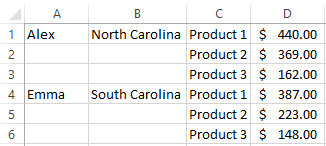
This is the small nameplate: only for this example and it could be filled in manually. But in practice, sometimes you have to fill in 30 thousand lines. To not fill this source table manually, you should create a formula to fill in Excel data by automatically. To do this, perform the series of sequential actions:
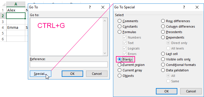
- Go to any empty cell in the source table.
- Select the tool: «HOME» – «Find and select» – «Go To» (or to press the hot keys CTRL + G).
- In the window that appears, click the «Special» button.
- In the window that appears, select the option «Blanks» and click OK. All empty cells are highlighted.
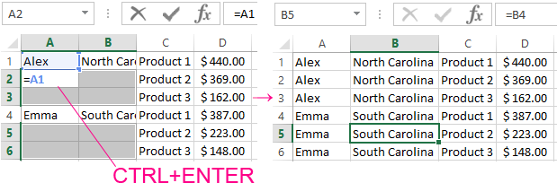
- Now enter the formula «=A1» and press CTRL + Enter. This is how the empty cells in Excel are filled with the previous value – automatically.
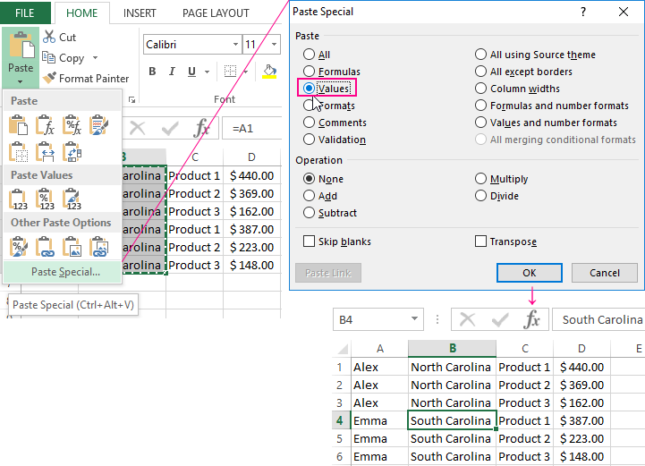
- Highlight the columns A:B and copy its contents.
- Select the tool: «HOME» – «Paste» – «Paste Special» (or press CTRL + ALT + V).
- In the window that appears, select the «Value» option and click OK. Now the original table is filled not just with formulas, but with natural values of the cells.
When filling 30 thousand lines it is impossible not to make mistakes. The above method not only saves forces and time, but also eliminates the occurrence of errors caused by the human factor.
Attention! In the 5-th paragraph, the table was beautifully filled without errors, since our active cell was at address A2, after completing the 4-th item. When using this method, be careful and watch where the active cell is after the selection. It is important where it will take its values.
Semi-automatic filling of the cells in Excel from the drop-down list
Now in semi-automatic mode you can fill the empty cells. There are only a few values that are repeated in sequential or in random order.
In the new source table, automatically fill in the columns C and D with the data corresponding to them.
- Fill in the column headings C1 – «Date» and D1 – «Payment Type».
- In the cell C2, enter the date 06/15/2018.
- In the cells C2:C4 the dates are repeated, therefore, you need to select the range C2:C4 and press CTRL+D to automatically fill the cells with the previous values.
- Enter the current date in the cell C5. To do this, press CTRL +; (the semicolon on the English keyboard layout). Fill in the current dates with the column C to the end of the table.
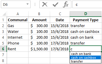
- The range of the cells D2:D4 you need to fill as shown below in the picture.
- In the cell D5 to enter the first letter «p», and then the word is not necessary to fill. It is enough to press the Enter key.
- In the cell D6, after entering the first letter «с», do not display part of the word for auto-fill. Therefore, you need to press ALT + ↓ (arrow down) to bring up the drop-down list. Select the value «cash on cashbox» in the arrow keys or the mouse pointer and press Enter.
This semiautomatic method of data entry allows several times to speed up and facilitate the process of working with tables.
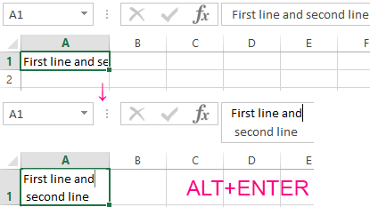
Attention! If the value consists of several lines, then when you press the ALT + (down arrow) combination, it will not be displayed in the drop-down list of values.
To split the value into strings using the ALT + Enter key combination. Thus, the text is divided into rows within the same cell.
Note. Notice how we entered the current date in step 4 using the hotkeys (CTRL +;). It is very convenient! And when you press CTRL + SHIFT +; we get the current time.
Filling
Filling makes your life easier and is used to fill ranges with values, so that you do not have to type manual entries.
Filling can be used for:
- Copying
- Sequences
- Dates
- Functions (*)
For now, do not think of functions. We will cover that in a later chapter.
How To Fill
Filling is done by selecting a cell, clicking the fill icon and selecting the range using drag and mark while holding the left mouse button down.
The fill icon is found in the button right corner of the cell and has the icon of a small square. Once you hover over it your mouse pointer will change its icon to a thin cross.
Click the fill icon and hold down the left mouse button, drag and mark the range that you want to cover.
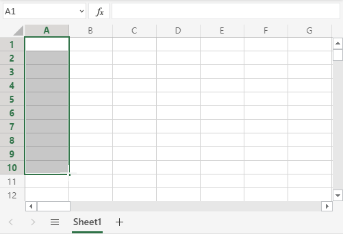
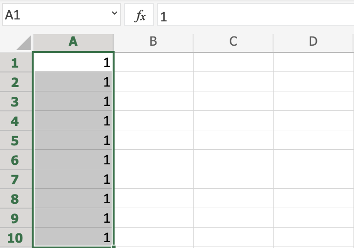
In this example, cell A1 was selected and the range A1:A10 was marked.
Now that we have learned how to fill. Let’s look into how to copy with the fill function.
Fill Copies
Filling can be used for copying. It can be used for both numbers and words.
Let’s have a look at numbers first.
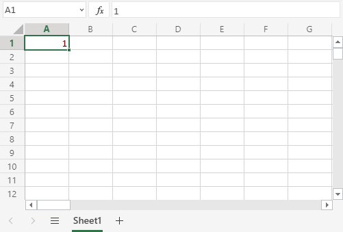
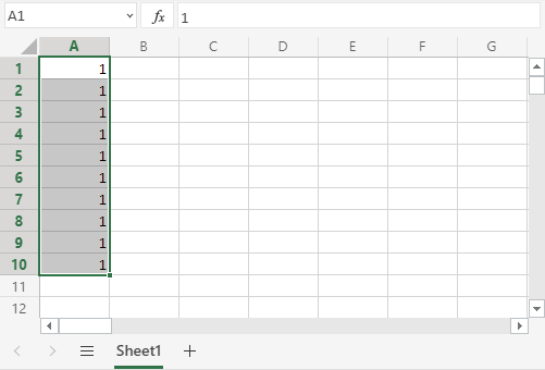
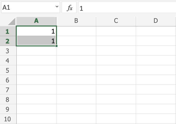
In this example we have typed the value A1(1):
Filling the range A1:A10 creates ten copies of
1:
The same principle goes for text.
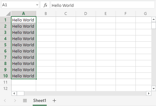
In this example we have typed A1(Hello World).
Filling the range A1:A10 creates ten copies of «Hello World»:
Now you have learned how to fill and to use it for copying both numbers and words. Let’s have a look at sequences.
Fill Sequences
Filling can be used to create sequences. A sequence is an order or a pattern. We can use the filling function to continue the order that has been set.
Sequences can for example be used on numbers and dates.
Let’s start with learning how to count from 1 to 10.
This is different from the last example because this time we do not want to copy, but to count from 1 to 10.
Start with typing A1(1):
First we will show an example which does not work, then we will do a working one. Ready?
Lets type the value (1) into the cell A2, which is what we have in A1. Now we have the same values in both A1 and A2.
Let’s use the fill function from A1:A10 to see what happens. Remember to mark both values before you fill the range.
What happened is that we got the same values as we did with copying. This is because the fill function assumes that we want to create copies as we had two of the same values in both the cells A1(1) and A2(1).
Change the value of A2(1) to A2(2). We now have two different values in the cells A1(1) and A2(2). Now, fill A1:A10
again. Remember to mark both the values (holding down shift) before you fill the
range:
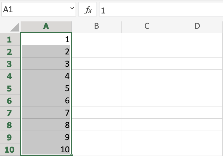
Congratulations! You have now counted from 1 to 10.
The fill function understands the pattern typed in the cells and continues it for us.
That is why it created copies when we had entered the value (1) in both cells,
as it saw no pattern. When we entered (1) and (2) in the cells it was able to understand the pattern and that the next cell A3 should be (3).
Let’s create another sequence. Type A1(2) and A2(4):
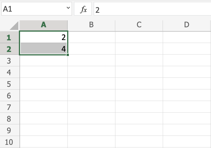
Now, fill A1:A10:
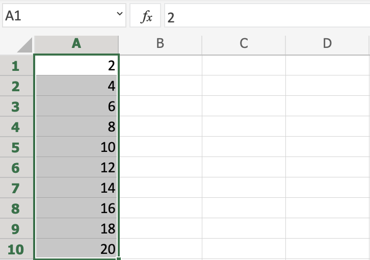
It counts from 2 to 20 in the range A1:A10.
This is because we created an order with A1(2) and A2(4).
Then it fills the next cells, A3(6), A4(8), A5(10) and so on. The fill function understands the pattern and helps us continue it.
Sequence of Dates
The fill function can also be used to fill dates.
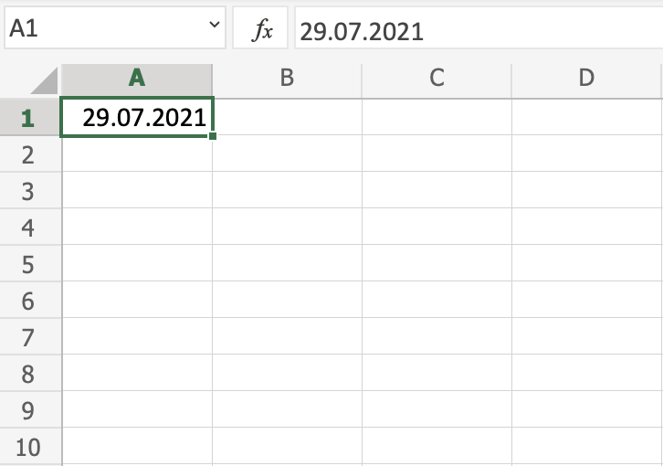
Test it by typing A1(29.07.2021):
And fill the range A1:A10:
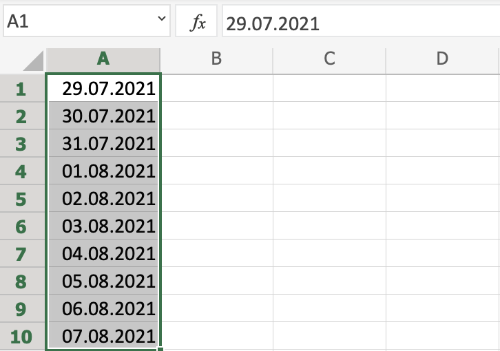
The fill function has filled 10 days from A1(29.07.2021) to A10(07.08.2021).
Note that it switched from July to August in cell A4. It knows the calendar and will count real dates.
Combining Words and Letters
Words and letters can also be combined.
Type A1(Hello 1) and A2(Hello 2):
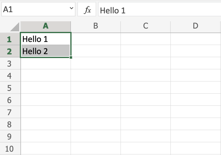
Next, fill A1:A10 to see what happens:
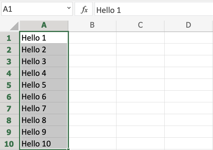
The result is that it counts from A1(Hello 1) to A10(Hello 10). Only the numbers have changed.
It recognised the pattern of the numbers and continued it for us. Words and numbers can be combined, as long as you use a recognizable pattern for the numbers.
Test Yourself With Exercises

The Fill Handle in Excel allows you to automatically fill in a list of data (numbers or text) in a row or column simply by dragging the handle. This can save you a lot of time when entering sequential data in large worksheets and make you more productive.
Instead of manually entering numbers, times, or even days of the week over and over again, you can use the AutoFill features (the fill handle or the Fill command on the ribbon) to fill cells if your data follows a pattern or is based on data in other cells. We’ll show you how to fill various types of series of data using the AutoFill features.
Fill a Linear Series into Adjacent Cells
One way to use the fill handle is to enter a series of linear data into a row or column of adjacent cells. A linear series consists of numbers where the next number is obtained by adding a “step value” to the number before it. The simplest example of a linear series is 1, 2, 3, 4, 5. However, a linear series can also be a series of decimal numbers (1.5, 2.5, 3.5…), decreasing numbers by two (100, 98, 96…), or even negative numbers (-1, -2, -3). In each linear series, you add (or subtract) the same step value.
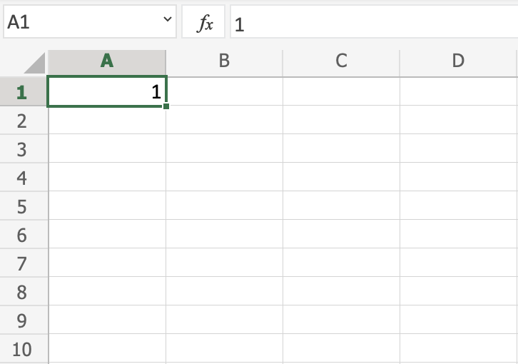
Let’s say we want to create a column of sequential numbers, increasing by one in each cell. You can type the first number, press Enter to get to the next row in that column, and enter the next number, and so on. Very tedious and time consuming, especially for large amounts of data. We’ll save ourselves some time (and boredom) by using the fill handle to populate the column with the linear series of numbers. To do this, type a 1 in the first cell in the column and then select that cell. Notice the green square in the lower-right corner of the selected cell? That’s the fill handle.

When you move your mouse over the fill handle, it turns into a black plus sign, as shown below.
With the black plus sign over the fill handle, click and drag the handle down the column (or right across the row) until you reach the number of cells you want to fill.
When you release the mouse button, you’ll notice that the value has been copied into the cells over which you dragged the fill handle.
Why didn’t it fill the linear series (1, 2, 3, 4, 5 in our example)? By default, when you enter one number and then use the fill handle, that number is copied to the adjacent cells, not incremented.
NOTE: To quickly copy the contents of a cell above the currently selected cell, press Ctrl+D, or to copy the contents of a cell to the left of a selected cell, press Ctrl+R. Be warned that copying data from an adjacent cell replaces any data that is currently in the selected cell.
To replace the copies with the linear series, click the “Auto Fill Options” button that displays when you’re done dragging the fill handle.
The first option, Copy Cells, is the default. That’s why we ended up with five 1s and not the linear series of 1–5. To fill the linear series, we select “Fill Series” from the popup menu.
The other four 1s are replaced with 2–5 and our linear series is filled.
You can, however, do this without having to select Fill Series from the Auto Fill Options menu. Instead of entering just one number, enter the first two numbers in the first two cells. Then, select those two cells and drag the fill handle until you’ve selected all the cells you want to fill.
Because you’ve given it two pieces of data, it will know the step value you want to use, and fill the remaining cells accordingly.
You can also click and drag the fill handle with the right mouse button instead of the left. You still have to select “Fill Series” from a popup menu, but that menu automatically displays when you stop dragging and release the right mouse button, so this can be a handy shortcut.
Fill a Linear Series into Adjacent Cells Using the Fill Command
If you’re having trouble using the fill handle, or you just prefer using commands on the ribbon, you can use the Fill command on the Home tab to fill a series into adjacent cells. The Fill command is also useful if you’re filling a large number of cells, as you’ll see in a bit.
To use the Fill command on the ribbon, enter the first value in a cell and select that cell and all the adjacent cells you want to fill (either down or up the column or to the left or right across the row). Then, click the “Fill” button in the Editing section of the Home tab.
Select “Series” from the drop-down menu.
On the Series dialog box, select whether you want the Series in Rows or Columns. In the Type box, select “Linear” for now. We will discuss the Growth and Date options later, and the AutoFill option simply copies the value to the other selected cells. Enter the “Step value”, or the increment for the linear series. For our example, we’re incrementing the numbers in our series by 1. Click “OK”.
The linear series is filled in the selected cells.
If you have a really long column or row you want to fill with a linear series, you can use the Stop value on the Series dialog box. To do this, enter the first value in the first cell you want to use for the series in the row or column, and click “Fill” on the Home tab again. In addition to the options we discussed above, enter the value into the “Stop value” box that you want as the last value in the series. Then, click “OK”.
In the following example, we put a 1 in the first cell of the first column and the numbers 2 through 20 will be entered automatically into the next 19 cells.
Fill a Linear Series While Skipping Rows
To make a full worksheet more readable, we sometimes skip rows, putting blank rows in between the rows of data. Even though there are blank rows, you can still use the fill handle to fill a linear series with blank rows.
To skip a row when filling a linear series, enter the first number in the first cell and then select that cell and one adjacent cell (for example, the next cell down in the column).
Then, drag the fill handle down (or across) until you fill the desired number of cells.
When you’re finished dragging the fill handle, you will see your linear series fills every other row.
If you want to skip more than one row, simply select the cell containing the first value and then select the number of rows you want to skip right after that cell. Then, drag the fill handle over the cells you want to fill.
You can also skip columns when you are filling across rows.
Fill Formulas into Adjacent Cells
You can also use the fill handle to propagate formulas to adjacent cells. Simply select the cell containing the formula you want to fill into adjacent cells and drag the fill handle down the cells in the column or across the cells in the row that you want to fill. The formula is copied to the other cells. If you used relative cell references, they will change accordingly to refer to the cells in their respective rows (or columns).
RELATED: Why Do You Need Formulas and Functions?
You can also fill formulas using the Fill command on the ribbon. Simply select the cell containing the formula and the cells you want to fill with that formula. Then, click “Fill” in the Editing section of the Home tab and select Down, Right, Up, or Left, depending on which direction you want to fill the cells.
RELATED: How to Manually Calculate Only the Active Worksheet in Excel
NOTE: The copied formulas will not recalculate, unless you have automatic workbook calculation enabled.
You can also use the keyboard shortcuts Ctrl+D and Ctrl+R, as discussed earlier, to copy formulas to adjacent cells.
Fill a Linear Series by Double Clicking on the Fill Handle
You can quickly fill a linear series of data into a column by double clicking the fill handle. When using this method, Excel only fills the cells in the column based on the longest adjacent column of data on your worksheet. An adjacent column in this context is any column that Excel encounters to the right or left of the column being filled, until a blank column is reached. If the columns directly on either side of the selected column are blank, you cannot use the double click method to fill the cells in the column. Also, by default, if some of the cells in the range of cells you’re filling already have data, only the empty cells above the first cell containing data are filled. For example, in the image below, there’s a value in cell G7 so when you double click on the fill handle on cell G2, the formula is only copied down through cell G6.
Fill a Growth Series (Geometric Pattern)
Up until now, we’ve been discussing filling linear series, where each number in the series is calculated by adding the step value to the previous number. In a growth series, or geometric pattern, the next number is calculated by multiplying the previous number by the step value.
There are two ways to fill a growth series, by entering the first two numbers and by entering the first number and the step value.
Method One: Enter the First Two Numbers in the Growth Series
To fill a growth series using the first two numbers, enter the two numbers into the first two cells of the row or column you want to fill. Right-click and drag the fill handle over as many cells as you want to fill. When you’re finished dragging the fill handle over the cells you want to fill, select “Growth Trend” from the popup menu that automatically displays.
NOTE: For this method, you must enter two numbers. If you don’t, the Growth Trend option will be grayed out.
Excel knows that the step value is 2 from the two numbers we entered in the first two cells. So, every subsequent number is calculated by multiplying the previous number by 2.
What if you want to start at a number other than 1 using this method? For example, if you wanted to start the above series at 2, you would enter 2 and 4 (because 2×2=4) in the first two cells. Excel would figure out that the step value is 2 and continue the growth series from 4 multiplying each subsequent number by 2 to get the next one in line.
Method Two: Enter the First Number in the Growth Series and Specify the Step Value
To fill a growth series based on one number and a step value, enter the first number (it doesn’t have to be 1) in the first cell and drag the fill handle over the cells you want to fill. Then, select “Series” from the popup menu that automatically displays.
On the Series dialog box, select whether your filling the Series in Rows or Columns. Under Type, select :”Growth”. In the “Step value” box, enter the value you want to multiply each number by to get the next value. In our example, we want to multiply each number by 3. Click “OK”.
The growth series is filled in the selected cells, each subsequent number being three times the previous number.
Fill a Series Using Built-in Items
So far, we’ve covered how to fill a series of numbers, both linear and growth. You can also fill series with items such as dates, days of the week, weekdays, months, or years using the fill handle. Excel has several built-in series that it can automatically fill.
The following image shows some of the series that are built in to Excel, extended across the rows. The items in bold and red are the initial values we entered and the rest of the items in each row are the extended series values. These built-in series can be filled using the fill handle, as we previously described for linear and growth series. Simply enter the initial values and select them. Then, drag the fill handle over the desired cells you want to fill.
Fill a Series of Dates Using the Fill Command
When filling a series of dates, you can use the Fill command on the ribbon to specify the increment to use. Enter the first date in your series in a cell and select that cell and the cells you want to fill. In the Editing section of the Home tab, click “Fill” and then select “Series”.
On the Series dialog box, the Series in option is automatically selected to match the set of cells you selected. The Type is also automatically set to Date. To specify the increment to use when filling the series, select the Date unit (Day, Weekday, Month, or Year). Specify the Step value. We want to fill the series with every weekday date, so we enter 1 as the Step value. Click “OK”.
The series is populated with dates that are only weekdays.
Fill a Series Using Custom Items
You can also fill a series with your own custom items. Say your company has offices in six different cities and you use those city names often in your Excel worksheets. You can add that list of cities as a custom list that will allow you to use the fill handle to fill the series once you enter the first item. To create a custom list, click the “File” tab.
On the backstage screen, click “Options” in the list of items on the left.
Click “Advanced” in the list of items on the left side of the Excel Options dialog box.
In the right panel, scroll down to the General section and click the “Edit Custom Lists” button.
Once you’re on the Custom Lists dialog box, there are two ways to fill a series of custom items. You can base the series on a new list of items you create directly on the Custom Lists dialog box, or on an existing list already on a worksheet in your current workbook. We will show you both methods.
Method One: Fill a Custom Series Based on a New List of Items
On the Custom Lists dialog box, make sure NEW LIST is selected in the Custom lists box. Click in the “List entries” box and enter the items in your custom lists, one item to a line. Be sure to enter the items in the order you want them filled into cells. Then, click “Add”.
The custom list is added to the Custom lists box, where you can select it so you can edit it by adding or removing items from the List entries box and clicking “Add” again, or you can delete the list by clicking “Delete”. Click “OK”.
Click “OK” on the Excel Options dialog box.
Now, you can type the first item in your custom list, select the cell containing the item and drag the fill handle over the cells you want to fill with the list. Your custom list is automatically filled into the cells.
Method Two: Fill a Custom Series Based on an Existing List of Items
Maybe you store your custom list on a separate worksheet in your workbook. You can import your list from the worksheet into the Custom Lists dialog box. To create a custom list based on an existing list on a worksheet, open the Custom Lists dialog box and make sure NEW LIST is selected in the Custom lists box, just like in the first method. However, for this method, click the cell range button to the right of the “Import list from cells” box.
Select the tab for the worksheet that contains your custom list at the bottom of the Excel window. Then, select the cells containing the items in your list. The name of the worksheet and the cell range are automatically entered into the Custom Lists edit box. Click the cell range button again to return to the full dialog box.
Now, click “Import”.
The custom list is added to the Custom lists box and you can select it and edit the list in the List entries box, if you want. Click “OK”. You can fill cells with your custom list using the fill handle, just like you did with the first method above.
The fill handle in Excel is a very useful feature if you create large worksheets that contain a lot of sequential data. You can save yourself a lot of time and tedium. Happy Filling!
READ NEXT
- › How to Use the YEAR Function in Microsoft Excel
- › How to Randomize a List in Microsoft Excel
- › How to AutoFill Dates in Microsoft Excel
- › How to Make a Simple Budget in Microsoft Excel
- › How to Create a Custom List in Microsoft Excel
- › How to Divide Numbers in Microsoft Excel
- › How to Multiply Columns in Microsoft Excel
- › Why the Right-Click Menu in Windows 11 Is Actually Good
Transcript
In this lesson, we’ll take a look at one of the most powerful tools in Excel, the fill handle. The fill handle allows you to fill cells with data that originates from one or more source cells. This data can be a straight copy of the source cells, or, it can be based on a repeatable pattern.
Let’s take a look.
The fill handle is a special box that appears in the lower right-hand corner of a selection. When you hover over the fill handle, you’ll see the cursor change from a white selection cross to a thin black cross. When you see the black cross, click and drag the handle over the cells you’d like to fill.
The fill handle can fill cells in four directions: right and left; up, down.
It also works when more than one cell is selected.
The fill handle will also recognize and repeat certain patterns. For example, you can use the fill handle to enter months and days of the week.
The fill handle will recognize the abbreviations as well.
The fill handle will also recognize and repeat numbers that appear with text. It understands how to count using first, second, third and so forth.
It knows how to increment things like item numbers or product codes.
Finally, the fill handle will increment dates automatically in both directions.

Author![]()
Dave Bruns
Hi — I’m Dave Bruns, and I run Exceljet with my wife, Lisa. Our goal is to help you work faster in Excel. We create short videos, and clear examples of formulas, functions, pivot tables, conditional formatting, and charts.