
Here is a quick trick for selecting empty cells.
- Pick the columns or rows where you want to fill in blanks.
- Press Ctrl + G or F5 to display the Go To dialog box.
- Click on the Special button. Note.
- Select the Blanks radio button and click OK.
How do you fill cells with the same formula?
Simply do the following:
- Select the cell with the formula and the adjacent cells you want to fill.
- Click Home > Fill, and choose either Down, Right, Up, or Left. Keyboard shortcut: You can also press Ctrl+D to fill the formula down in a column, or Ctrl+R to fill the formula to the right in a row.
How do you write text in a formula such as when comparing a text field A1 =< some text >)?
This example shows two ways to compare text strings in Excel….Compare Text
- Use the EXACT function (case-sensitive).
- Use the formula =A1=B1 (case-insensitive).
- Add the IF function to replace TRUE and FALSE with a word or message.
- Do you want to compare two or more columns by highlighting the differences in each row?
How do you use an IF function?
Use the IF function, one of the logical functions, to return one value if a condition is true and another value if it’s false. For example: =IF(A2>B2,”Over Budget”,”OK”) =IF(A2=B2,B4-A4,””)
What do you need to include when you are entering text into your formula?
We often hear that you want to make data easier to understand by including text in your formulas, such as “2,347 units sold.” To include text in your functions and formulas, surround the text with double quotes (“”).
How can I have text and formula in the same cell?
Combine Cells With Text and a Number
- Select the cell in which you want the combined data.
- Type the formula, with text inside double quotes. For example: =”Due in ” & A3 & ” days” NOTE: To separate the text strings from the numbers, end or begin the text string with a space.
- Press Enter to complete the formula.
How do I add text to the end of a formula in Excel?
Add specified text to the beginning / end of all cells with formulas
- If you want to add other specified text in each cell, just replace the Class A: with your text in both formulas.
- The formulas of =A2 & “: Class A” and =Concatenate (A2, “: Class A”) will add : Class A at the end of the cells.
How do I use Excel formulas in Word?
Insert a formula in a table cell
- Select the table cell where you want your result. If the cell is not empty, delete its contents.
- On the Table Tools, Layout tab, in the Data group, click Formula.
- Use the Formula dialog box to create your formula.
How do I add a formula to all values in Word?
Sum a column or row of numbers in a table
- Click the table cell where you want your result to appear.
- On the Layout tab (under Table Tools), click Formula.
- In the Formula box, check the text between the parentheses to make sure Word includes the cells you want to sum, and click OK. =SUM(ABOVE) adds the numbers in the column above the cell you’re in.
How do I write formulas in Word?
Write an equation or formula
- Choose Insert > Equation and choose the equation you want from the gallery.
- After you insert the equation the Equation Tools Design tab opens with symbols and structures that can be added to your equation.
How do you show the formulas in Word?
Insert Equations in Word: Instructions
- To insert a preset equation in Word, place your cursor at insertion point in your document where you want the equation to appear.
- Then click the “Insert” tab in the Ribbon.
- Then click the “Equation” button in the “Symbols” button group on the right end of the tab.
How do I write exponents in Word?
Click anywhere in the equation box and type in the number or formula you want to appear before the exponent, then type in a caret (“^”), which tells Word that whatever comes after the caret will be part of the exponent.
What is the equation for a line with no slope?
If you think about the slope formula, y = mx + b, if m = 0, then y = 0x+b, and if you multiply anything by 0, it disappears, so zero slope gives y = b. If it is x= #, it is a vertical line through whatever value o x you have.
This example demonstrates how to fill data gaps in an excel file.
Question from the customer:
Currently, we are testing the Advanced ETL Processor tool and evaluating how we can use it best for our specific cases. Recently we have come across a problem:
Sometimes it is necessary to fill columns in excel, only if a certain value, for example, the order number is given in the destination file.
In this very example, which you can see in the attachments, I would like to have AETLP check, if the order number in the destination file meets an order number in the source file.
And if so, I would like to have AETLP to fill the empty gaps, in this case, name and description for example, but only if they’re empty.
Data example

Original forum post
The solution
The simplest way to transform the data is to use the Lookup transformation function.

Transformation

How it works
- Lookup loads data from excel file
- When the matched value is found lookup returns Name and Description fields values otherwise it returns nulls
- «If Null or Empty string» transformation function fills the gaps: EG when Name is missing it takes value from the lookup otherwise it uses the original value
Lookup Mapping: Input fields

Lookup Mapping: Output fields

To view the example follow the steps below
- Download and install Advanced ETL Processor [Link]
- Download and Unzip example[Link]
- Create a new transformation and open the .ats file
- Double click on the Reader object and amend the source file path
- Double click on the Transformer object
- Double click on the Lookup object and amend the source file path
- Double click on the Writer object and amend the target file path
- Press the green arrow to run the transformation
Note: That reader and writer point to the same file
Please contact us if you need help with transforming the data
What’s the best way to fill in the gaps in a spreadsheet column that looks like this?

So that each row would be an accurately-divided step between the first and last value in the column? I don’t want to have to manually add and divide each step.
Edit
The results I’m after would divide the difference by 18 because there are 18 cells between the top and bottom value, and insert the difference into each cell.
i.e.: the second cell in the screenshot would have the formula:
= 0.2151452046 + ((0.235 - 0.2151452046) / 18) (which equals 0.2361030442)
The third cell would then be:
= 0.2361030442 + ((0.235 - 0.2151452046) / 18)
Does that make sense? I don’t know how better to explain it. Thanks.
Second edit
Here’s the numbers with a manual formula that takes the previous value and adds the difference between the bottom and the top and divides it by the number of cells between:

I have data in consecutive cells in a column in Sheet_2.
(In my case, they happen to be dates that are approximately a month apart,
but this is probably unimportant.)
Something like this:
| A | B | |
|---|---|---|
| 1 | Start of Period | |
| 2 | ||
| 3 | … | 30-Dec-2019 |
| 4 | … | 30-Jan-2020 |
| 5 | … | 2-Mar-2020 |
I want to fill in a column on Sheet_1
with references to these values on Sheet_2.
To clarify: I want to auto-fill formulas in Sheet1 that reference Sheet2.
Each value should be repeated three times, followed by a gap (blank cell).
It should look like this:
| A | B | C | D | |
|---|---|---|---|---|
| 1 | {} |
|||
| 2 | Cheque A | Cheque N | Date | Inclusive |
| 3 | 11150 | 30-Dec-2019 | x | |
| 4 | 30-Dec-2019 | x | ||
| 5 | 30-Dec-2019 | x | ||
| 6 | ||||
| 7 | 11150 | 30-Jan-2020 | x | |
| 8 | 30-Jan-2020 | x | ||
| 9 | 30-Jan-2020 | x | ||
| 10 | ||||
| 11 | 11150 | 2-Mar-2020 | x | |
| 12 | 2-Mar-2020 | x | ||
| 13 | 2-Mar-2020 | x | ||
| 14 |
but it should actually be references, like this:
| A | B | C | D | |
|---|---|---|---|---|
| 1 | … | |||
| 2 | … | … | Date | … |
| 3 | … | =sheet2!B3 | ||
| 4 | =sheet2!B3 | |||
| 5 | =sheet2!B3 | |||
| 6 | blank | |||
| 7 | … | =sheet2!B4 | ||
| 8 | =sheet2!B4 | |||
| 9 | =sheet2!B4 | |||
| 10 | blank | |||
| 11 | … | =sheet2!B5 | ||
| 12 | =sheet2!B5 | |||
| 13 | =sheet2!B5 | |||
| 14 | blank |
At present, if I reference it manually and then drag and fill,
it skips a bunch of rows.
I’ve tried a couple of variations of INDIRECT,
but I must be using it incorrectly as I can’t get it to work.
Any help is greatly appreciated.
![]()
asked Jun 18, 2021 at 15:47
![]()
2
Assuming that you always want Sheet_1 to have groups of three:
In Sheet_1!C3, enter
=INDEX(Sheet_2!B$3:B$99, INT((ROW()-ROW($C$3))/4)+1, 1)
replacing 99 with the last row where Sheet_2!B has data.
Copy that formula into cells C4 and C5.
Leave C6 blank.
Select cells C3:C6 and drag/fill down.
answered Jun 19, 2021 at 18:28
![]()
1
This formula:
=IF(ROUNDUP((ROW()-2)/4,0) = (ROW()-2)/4,"",INDIRECT("Sheet2!A"&(ROUND(ROW()/4,0)+1)))
Will take dates in Sheet2 and place each one on three rows on Sheet1, followed by a blank cell before the next date repeated three times, and so on.
answered Jun 18, 2021 at 17:01
![]()
1
Oct 28 2019
04:38 AM
Fill in gap between dates in a table
I have table with several dates in a column and numbers in another. I want to fill the gap between the missing days using weekdays only, and repeat the number on each of the dates already available in the date column. How do I do this? Thanks
Here is the table to fill
|
Date |
Value |
|
6/30/1980 |
1 |
|
12/12/1980 |
0 |
|
12/26/1980 |
1 |
|
1/8/1981 |
0 |
|
2/9/1981 |
1 |
|
6/22/1981 |
0 |
Bottom Line: In this post we look at 3 ways to copy down values in blank cells in a column. The techniques include using a formula, Power Query, and a VBA macro.
Skill Level: Intermediate
Watch the Tutorial
Download the Excel Files
You can download both the BEGIN and FINAL files if you want to follow along and practice.
Filling Down Blank Cells
Excel makes it easy to fill down, or copy down, a value into the cells below. You can simply double-click or drag down the fill handle for the cell that you want copied, to populate the cells below it with the same value.
But is there an easy way to replicate that process hundreds of times for reports that have large amounts of data?
In this post we’ll look at three ways to automate this process with: a simple formula, Power Query, and a VBA macro.
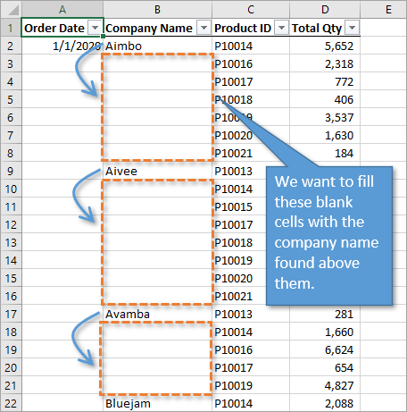
1. Filling Down Using a Formula
The first way to solve this problem is by using a very simple formula in all of the blank cells that references the cell above. Here are the steps.
Step 1: Select the Blank Cells
In order to select the blank cells in a column and fill them with a formula, we start by selecting all of the cells (including the populated cells). There are many ways to do this, including holding the Shift key down while you navigate to the bottom of your column, or if your data is in an Excel Table, using the keyboard shortcut Ctrl+Space.
Checkout my posts on 7 Keyboard Shortcuts for Selecting Cells and Ranges in Excel and 5 Keyboard Shortcuts for Rows and Columns in Excel to learn more.
With all of those cells selected, we can pare down our selection to include only the blank cells. This is done by using the Go To Special window from the Find & Select menu on the Home tab of the ribbon.
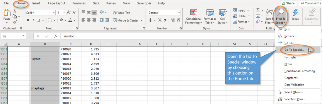
An alternative is to open the Go To window using F5 or Ctrl+G. Then press the Special button for the Go To Special window.
Once the Go To Special window is open, you can choose the option that says Blanks. This will select only the blank cells from the current selection.
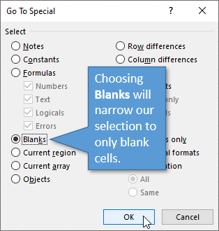
When you hit OK, you’ll notice that the cells that have values in them are no longer selected.
Step 2: Write the Formula
From here you can start typing the formula, which is very simple. Type the equals sign (=) and then reference the cell above (in the case of our example, B2). That’s all you need for the formula!
Step 3: Ctrl+Enter the Formula
After writing the formula, don’t just hit Enter. Instead, use Ctrl+Enter to fill all of the selected cells with the same formula. Hold the Ctrl key, then hit Enter.
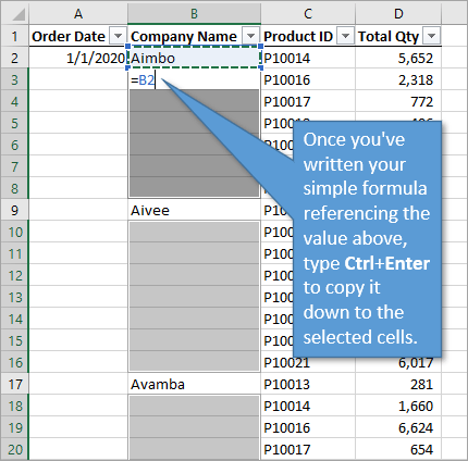
Because your formula reference is relative (B2), not absolute ($B$2), each cell will simply copy the value for the cell directly above it.
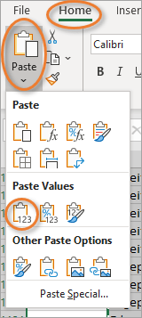
Step 4: Copy & Paste Values
It is a good idea to now copy the entire data column and then paste over it using the Paste Values option so that the data is hard coded. Then, if you do any sorting, the data will not change. You can find the Paste Values option on the Home tab in the Paste drop-down menu:
There are other ways to paste values, including the right-click menu or using keyboard shortcuts. These posts explain those options:
Paste Values with the Right-click & Drag Mouse Shortcut
5 Keyboard Shortcuts to Paste Values in Excel
2. Filling Down Using Power Query
For this option, your data should be in Excel Table format. From anywhere inside the table, you can select the Data or Power Query tab, and then select From Table/Range. You can also create a query that connects to a different data source like a database or the web.
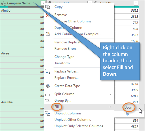
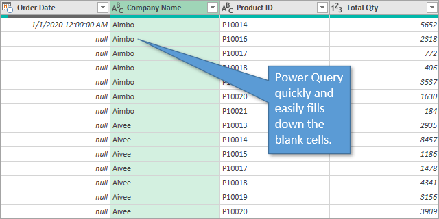
This opens up the Power Query Editor. In Power Query, the blank cells are labeled as null in each cell.
To fill down, just right-click on the column header and select Fill and then Down.
Power Query will fill down each section of blank cells in the column with the value from the cell above it.
When you click on Close & Load, a new sheet will be added to the workbook with these changes.
This process of filling down can be done for multiple columns simultaneously by first selecting multiple columns with Ctrl or Shift, then performing the Fill > Down operation.
If Power Query is somewhat new to you, I invite you to check out this post: Power Query Overview: An Introduction to Excel’s Most Powerful Data Tool.
Free Webinar on Power Query, VBA, & More
I also have a free webinar running right now that covers an introduction to Power Query and the other Excel tools like Power Pivot, Power BI, Macros & VBA, pivot tables, and more.

Click here to register for the webinar
3. Filling Down Using a Macro
To fill down using a macro, start by opening the VB Editor. You can do this by going to the Developer tab and clicking on the Visual Basic button or by using the keyboard shortcut Alt+F11. Insert a new code module, and then write your macro.
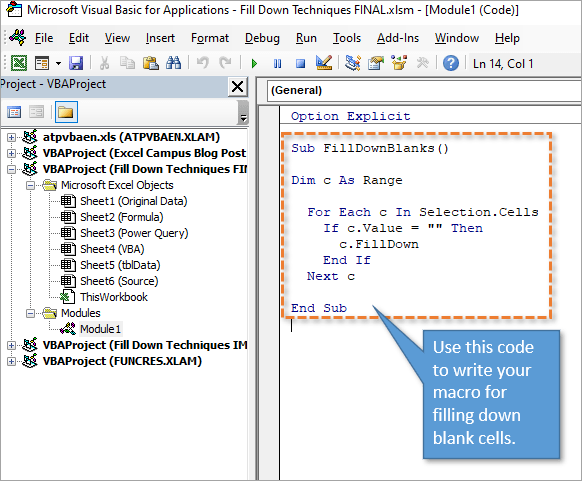
This macro loops through all of the cells in the selected range and performs the FillDown method if the cell is blank. The FillDown method copies the value from the cell above.
If this is a macro that you could use frequently, you might want to consider adding this macro to your personal Macro Workbook and creating a customized button for it. That’s what I’ve done and it looks like this on my Ribbon.
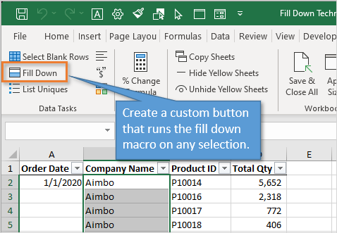
For instruction on how to create a Personal Macro Workbook and custom Ribbon buttons, check out this tutorial: How to Create a Personal Macro Workbook (Video Series).
Pros and Cons
So which of these three methods are right for you? Consider these things:
- The formula method is simple and easy to implement. It can be done without any knowledge of Power Query or VBA. However, it’s not as quick as a one-click button solution.
- Power Query requires source data that outputs into a separate worksheet, so it’s more of a process than simply filling down blank cells. If you are already data cleansing on a regular basis for other things, adding this to your existing process might make more sense.
- Once the initial macro is set up, VBA is a quick solution that’s easy to use—just click a button. However, there is a big disadvantage of this method. You aren’t able to undo your action once that button has been pushed, so you would have to be sure to save a backup copy beforehand if that is a concern for you.
Conclusion
There are three different methods for a very common Excel task. Did I miss any? Please leave a comment below if you have another way to go about it, or have any questions. Thanks! 🙂
I love learning new things. Today I was using a CSV export of data in Excel and was just using Excel to reassemble the data. At one point it resembled something like:

This is, of course, after some manipulation. Basically I removed the parts of a URL column expanded by delimiter (“/”) I didn’t want. This left awkward gaps and all I wanted was to quickly delete the gaps and shift contents of remaining cells to the left to sort of “reconstruct” each row without gaps. Since they didn’t line up in neat columns, I needed a different method.
I found a great article that helped. To summarize the steps:
- Select the range for which you’ll delete blank cells and shift data left.
- Press Ctrl+G.
- Click Special… (lower left of dialog)
- Choose the Blanks radio button
- Click OK.
- All blank cells in the selected range remain highlighted. Now right-click any of the selected blank cells.
- Choose Delete.
- Select Shift cells left.
- Click OK.
Here’s an animated GIF showing the process on my example data:

-
11-24-2010, 12:29 PM
#1

Registered User
Trying to fill in the gaps
Hi,
I’m trying to get Excel to save me some time filling in years between a start year and an end year.
Basically I have a column of start years, and a column of end years, and I need a column of all the years in-between seperated by pipes.
So, we should have something like:
Cell 1: 1975
Cell 2: 1980
Cell 3: 1975|1976|1977|1978|1979|1980I have about 700 of these so any help would be much appreciated!
-
11-24-2010, 01:08 PM
#2
Registered User
Re: Trying to fill in the gaps
Do you have always the same 5 year difference between the start and the end year? If don’t, is there a (theoretical) maximum number of difference?
An example file is never useless!
Tried an example function of mine and got errors?
— Had you found them, replace ; with , and , with .
-
11-24-2010, 01:11 PM
#3
Re: Trying to fill in the gaps
this is one way with functions max range 1991-2011 ie a 21 year span
-
11-24-2010, 01:17 PM
#4
Re: Trying to fill in the gaps
Assuming the start year(s) are in column A and the end year(s) are in column B, one way:
The output will be in column C
Regards
Trevor Shuttleworth — Excel Aid
I dream of a better world where chickens can cross the road without having their motives questioned
‘Being unapologetic means never having to say you’re sorry’ John Cooper Clarke
-
11-24-2010, 01:29 PM
#5
Registered User
Re: Trying to fill in the gaps
Yeah I was also working with a little macro with accessory cols. It has a 20 year limit as well.
Edit: never mind. It has a bug
Last edited by KiPA; 11-24-2010 at 01:35 PM.
Reason: Fail
-
11-24-2010, 01:41 PM
#6
Registered User
Re: Trying to fill in the gaps
-
11-24-2010, 02:37 PM
#7
Re: Trying to fill in the gaps
There’s no limit with the code I provided. No helper columns either.
Regards
-
11-24-2010, 07:53 PM
#8
Re: Trying to fill in the gaps
ok a udf use as =unconcat(a1,b1)
-
11-25-2010, 07:59 AM
#9
Registered User
Re: Trying to fill in the gaps
Thank you so much guys. There are so many great solutions, I don’t know which one to use first!
-
11-25-2010, 09:02 AM
#10
Re: Trying to fill in the gaps
You’re welcome. Thanks for the feedback.
-
11-25-2010, 02:47 PM
#11
Registered User
Re: Trying to fill in the gaps
Glad to help
—
Originally Posted by martindwilson
ok a udf use as =unconcat(a1,b1)
I have ; separator with functions but I’m not sure how I have to use them when dealing with custom functions. I cannot get this working and I’ve tried all four considerable alternatives: a) , at cell and at code, b) ; at cell and at code, c) ; at cell and , at code, d) , at cell and ; at code.
Any advices?
-
11-25-2010, 08:05 PM
#12
Re: Trying to fill in the gaps
-
11-26-2010, 05:15 AM
#13
Registered User
Re: Trying to fill in the gaps
Yeah that didn’t help. I strongly believe that the solution is related to that first code row. See, if I change the code so that the separator would be ; the editor reminds me: «Expected: list separator or )» so the separator must be comma (,). When I look the udf cell it yells «#NAME?»
So if I change the udf from =unconcat(A1;B1) to =unconcat(A1,B1) I got «The formula you typed contains an error.» which usually in simple cases like this is because I used , separator instead of expected ;But! Thanks anyway! I’ll try to find (typical) udf separator problems with search engines.
-
11-26-2010, 05:24 AM
#14
Registered User
Re: Trying to fill in the gaps
Can someone please help me with this… I need this bit urgent.. Sorry if i disturbed anyone.. I am new.
http://www.excelforum.com/excel-new-…-attached.html
-
11-26-2010, 06:18 AM
#15
Registered User
Re: Trying to fill in the gaps
-
11-26-2010, 08:19 AM
#16
Re: Trying to fill in the gaps
better still follow the rules ands start your own thread


