
Excel for iPad Excel for iPhone Excel for Android tablets Excel for Android phones Excel Mobile More…Less
If you need to duplicate an entry in several adjacent cells or you want to create a table that lists the months of the year in the first row, you can fill the data and avoid repetitive typing.
To fill cells in Excel Mobile for Windows 10, Excel for Android tablets or phones, or Excel for iPads or iPhones, you first tap a cell, row, or column that you want to fill into other cells. Then you tap it again, tap Fill, and then drag a green fill handle to the cells you want to fill.
Here’s a little more information on how to do this.
-
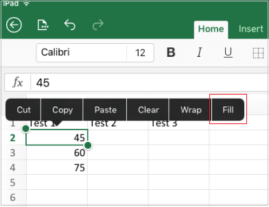
Tap to select the cell that contains the data you want to fill into other cells, and then tap the cell a second time to open the Edit menu.

-
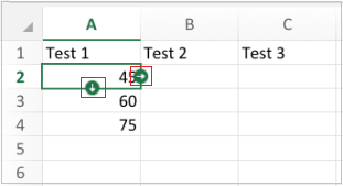
Tap Fill, and then tap and drag the fill arrows down or to the right.
-
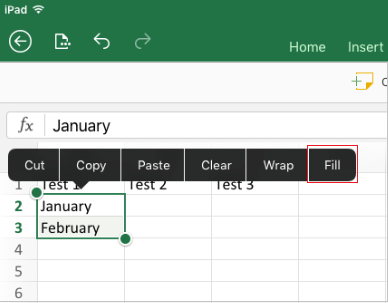
Type a starting value for the series.
-
Type a value in the next cell either below or to the right to establish a pattern.
-
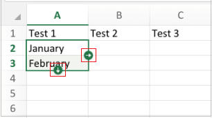
Tap to select the first cell, and then drag the selection handle around the second value.
-
On the Edit menu, tap Fill, and then tap and drag the fill arrow down.
Top of Page
Need more help?
Want more options?
Explore subscription benefits, browse training courses, learn how to secure your device, and more.
Communities help you ask and answer questions, give feedback, and hear from experts with rich knowledge.

The Fill Handle in Excel allows you to automatically fill in a list of data (numbers or text) in a row or column simply by dragging the handle. This can save you a lot of time when entering sequential data in large worksheets and make you more productive.
Instead of manually entering numbers, times, or even days of the week over and over again, you can use the AutoFill features (the fill handle or the Fill command on the ribbon) to fill cells if your data follows a pattern or is based on data in other cells. We’ll show you how to fill various types of series of data using the AutoFill features.
Fill a Linear Series into Adjacent Cells
One way to use the fill handle is to enter a series of linear data into a row or column of adjacent cells. A linear series consists of numbers where the next number is obtained by adding a “step value” to the number before it. The simplest example of a linear series is 1, 2, 3, 4, 5. However, a linear series can also be a series of decimal numbers (1.5, 2.5, 3.5…), decreasing numbers by two (100, 98, 96…), or even negative numbers (-1, -2, -3). In each linear series, you add (or subtract) the same step value.
Let’s say we want to create a column of sequential numbers, increasing by one in each cell. You can type the first number, press Enter to get to the next row in that column, and enter the next number, and so on. Very tedious and time consuming, especially for large amounts of data. We’ll save ourselves some time (and boredom) by using the fill handle to populate the column with the linear series of numbers. To do this, type a 1 in the first cell in the column and then select that cell. Notice the green square in the lower-right corner of the selected cell? That’s the fill handle.

When you move your mouse over the fill handle, it turns into a black plus sign, as shown below.
With the black plus sign over the fill handle, click and drag the handle down the column (or right across the row) until you reach the number of cells you want to fill.
When you release the mouse button, you’ll notice that the value has been copied into the cells over which you dragged the fill handle.
Why didn’t it fill the linear series (1, 2, 3, 4, 5 in our example)? By default, when you enter one number and then use the fill handle, that number is copied to the adjacent cells, not incremented.
NOTE: To quickly copy the contents of a cell above the currently selected cell, press Ctrl+D, or to copy the contents of a cell to the left of a selected cell, press Ctrl+R. Be warned that copying data from an adjacent cell replaces any data that is currently in the selected cell.
To replace the copies with the linear series, click the “Auto Fill Options” button that displays when you’re done dragging the fill handle.
The first option, Copy Cells, is the default. That’s why we ended up with five 1s and not the linear series of 1–5. To fill the linear series, we select “Fill Series” from the popup menu.
The other four 1s are replaced with 2–5 and our linear series is filled.
You can, however, do this without having to select Fill Series from the Auto Fill Options menu. Instead of entering just one number, enter the first two numbers in the first two cells. Then, select those two cells and drag the fill handle until you’ve selected all the cells you want to fill.
Because you’ve given it two pieces of data, it will know the step value you want to use, and fill the remaining cells accordingly.
You can also click and drag the fill handle with the right mouse button instead of the left. You still have to select “Fill Series” from a popup menu, but that menu automatically displays when you stop dragging and release the right mouse button, so this can be a handy shortcut.
Fill a Linear Series into Adjacent Cells Using the Fill Command
If you’re having trouble using the fill handle, or you just prefer using commands on the ribbon, you can use the Fill command on the Home tab to fill a series into adjacent cells. The Fill command is also useful if you’re filling a large number of cells, as you’ll see in a bit.
To use the Fill command on the ribbon, enter the first value in a cell and select that cell and all the adjacent cells you want to fill (either down or up the column or to the left or right across the row). Then, click the “Fill” button in the Editing section of the Home tab.
Select “Series” from the drop-down menu.
On the Series dialog box, select whether you want the Series in Rows or Columns. In the Type box, select “Linear” for now. We will discuss the Growth and Date options later, and the AutoFill option simply copies the value to the other selected cells. Enter the “Step value”, or the increment for the linear series. For our example, we’re incrementing the numbers in our series by 1. Click “OK”.
The linear series is filled in the selected cells.
If you have a really long column or row you want to fill with a linear series, you can use the Stop value on the Series dialog box. To do this, enter the first value in the first cell you want to use for the series in the row or column, and click “Fill” on the Home tab again. In addition to the options we discussed above, enter the value into the “Stop value” box that you want as the last value in the series. Then, click “OK”.
In the following example, we put a 1 in the first cell of the first column and the numbers 2 through 20 will be entered automatically into the next 19 cells.
Fill a Linear Series While Skipping Rows
To make a full worksheet more readable, we sometimes skip rows, putting blank rows in between the rows of data. Even though there are blank rows, you can still use the fill handle to fill a linear series with blank rows.
To skip a row when filling a linear series, enter the first number in the first cell and then select that cell and one adjacent cell (for example, the next cell down in the column).
Then, drag the fill handle down (or across) until you fill the desired number of cells.
When you’re finished dragging the fill handle, you will see your linear series fills every other row.
If you want to skip more than one row, simply select the cell containing the first value and then select the number of rows you want to skip right after that cell. Then, drag the fill handle over the cells you want to fill.
You can also skip columns when you are filling across rows.
Fill Formulas into Adjacent Cells
You can also use the fill handle to propagate formulas to adjacent cells. Simply select the cell containing the formula you want to fill into adjacent cells and drag the fill handle down the cells in the column or across the cells in the row that you want to fill. The formula is copied to the other cells. If you used relative cell references, they will change accordingly to refer to the cells in their respective rows (or columns).
RELATED: Why Do You Need Formulas and Functions?
You can also fill formulas using the Fill command on the ribbon. Simply select the cell containing the formula and the cells you want to fill with that formula. Then, click “Fill” in the Editing section of the Home tab and select Down, Right, Up, or Left, depending on which direction you want to fill the cells.
RELATED: How to Manually Calculate Only the Active Worksheet in Excel
NOTE: The copied formulas will not recalculate, unless you have automatic workbook calculation enabled.
You can also use the keyboard shortcuts Ctrl+D and Ctrl+R, as discussed earlier, to copy formulas to adjacent cells.
Fill a Linear Series by Double Clicking on the Fill Handle
You can quickly fill a linear series of data into a column by double clicking the fill handle. When using this method, Excel only fills the cells in the column based on the longest adjacent column of data on your worksheet. An adjacent column in this context is any column that Excel encounters to the right or left of the column being filled, until a blank column is reached. If the columns directly on either side of the selected column are blank, you cannot use the double click method to fill the cells in the column. Also, by default, if some of the cells in the range of cells you’re filling already have data, only the empty cells above the first cell containing data are filled. For example, in the image below, there’s a value in cell G7 so when you double click on the fill handle on cell G2, the formula is only copied down through cell G6.
Fill a Growth Series (Geometric Pattern)
Up until now, we’ve been discussing filling linear series, where each number in the series is calculated by adding the step value to the previous number. In a growth series, or geometric pattern, the next number is calculated by multiplying the previous number by the step value.
There are two ways to fill a growth series, by entering the first two numbers and by entering the first number and the step value.
Method One: Enter the First Two Numbers in the Growth Series
To fill a growth series using the first two numbers, enter the two numbers into the first two cells of the row or column you want to fill. Right-click and drag the fill handle over as many cells as you want to fill. When you’re finished dragging the fill handle over the cells you want to fill, select “Growth Trend” from the popup menu that automatically displays.
NOTE: For this method, you must enter two numbers. If you don’t, the Growth Trend option will be grayed out.
Excel knows that the step value is 2 from the two numbers we entered in the first two cells. So, every subsequent number is calculated by multiplying the previous number by 2.
What if you want to start at a number other than 1 using this method? For example, if you wanted to start the above series at 2, you would enter 2 and 4 (because 2×2=4) in the first two cells. Excel would figure out that the step value is 2 and continue the growth series from 4 multiplying each subsequent number by 2 to get the next one in line.
Method Two: Enter the First Number in the Growth Series and Specify the Step Value
To fill a growth series based on one number and a step value, enter the first number (it doesn’t have to be 1) in the first cell and drag the fill handle over the cells you want to fill. Then, select “Series” from the popup menu that automatically displays.
On the Series dialog box, select whether your filling the Series in Rows or Columns. Under Type, select :”Growth”. In the “Step value” box, enter the value you want to multiply each number by to get the next value. In our example, we want to multiply each number by 3. Click “OK”.
The growth series is filled in the selected cells, each subsequent number being three times the previous number.
Fill a Series Using Built-in Items
So far, we’ve covered how to fill a series of numbers, both linear and growth. You can also fill series with items such as dates, days of the week, weekdays, months, or years using the fill handle. Excel has several built-in series that it can automatically fill.
The following image shows some of the series that are built in to Excel, extended across the rows. The items in bold and red are the initial values we entered and the rest of the items in each row are the extended series values. These built-in series can be filled using the fill handle, as we previously described for linear and growth series. Simply enter the initial values and select them. Then, drag the fill handle over the desired cells you want to fill.
Fill a Series of Dates Using the Fill Command
When filling a series of dates, you can use the Fill command on the ribbon to specify the increment to use. Enter the first date in your series in a cell and select that cell and the cells you want to fill. In the Editing section of the Home tab, click “Fill” and then select “Series”.
On the Series dialog box, the Series in option is automatically selected to match the set of cells you selected. The Type is also automatically set to Date. To specify the increment to use when filling the series, select the Date unit (Day, Weekday, Month, or Year). Specify the Step value. We want to fill the series with every weekday date, so we enter 1 as the Step value. Click “OK”.
The series is populated with dates that are only weekdays.
Fill a Series Using Custom Items
You can also fill a series with your own custom items. Say your company has offices in six different cities and you use those city names often in your Excel worksheets. You can add that list of cities as a custom list that will allow you to use the fill handle to fill the series once you enter the first item. To create a custom list, click the “File” tab.
On the backstage screen, click “Options” in the list of items on the left.
Click “Advanced” in the list of items on the left side of the Excel Options dialog box.
In the right panel, scroll down to the General section and click the “Edit Custom Lists” button.
Once you’re on the Custom Lists dialog box, there are two ways to fill a series of custom items. You can base the series on a new list of items you create directly on the Custom Lists dialog box, or on an existing list already on a worksheet in your current workbook. We will show you both methods.
Method One: Fill a Custom Series Based on a New List of Items
On the Custom Lists dialog box, make sure NEW LIST is selected in the Custom lists box. Click in the “List entries” box and enter the items in your custom lists, one item to a line. Be sure to enter the items in the order you want them filled into cells. Then, click “Add”.
The custom list is added to the Custom lists box, where you can select it so you can edit it by adding or removing items from the List entries box and clicking “Add” again, or you can delete the list by clicking “Delete”. Click “OK”.
Click “OK” on the Excel Options dialog box.
Now, you can type the first item in your custom list, select the cell containing the item and drag the fill handle over the cells you want to fill with the list. Your custom list is automatically filled into the cells.
Method Two: Fill a Custom Series Based on an Existing List of Items
Maybe you store your custom list on a separate worksheet in your workbook. You can import your list from the worksheet into the Custom Lists dialog box. To create a custom list based on an existing list on a worksheet, open the Custom Lists dialog box and make sure NEW LIST is selected in the Custom lists box, just like in the first method. However, for this method, click the cell range button to the right of the “Import list from cells” box.
Select the tab for the worksheet that contains your custom list at the bottom of the Excel window. Then, select the cells containing the items in your list. The name of the worksheet and the cell range are automatically entered into the Custom Lists edit box. Click the cell range button again to return to the full dialog box.
Now, click “Import”.
The custom list is added to the Custom lists box and you can select it and edit the list in the List entries box, if you want. Click “OK”. You can fill cells with your custom list using the fill handle, just like you did with the first method above.
The fill handle in Excel is a very useful feature if you create large worksheets that contain a lot of sequential data. You can save yourself a lot of time and tedium. Happy Filling!
READ NEXT
- › How to Use the YEAR Function in Microsoft Excel
- › How to Randomize a List in Microsoft Excel
- › How to AutoFill Dates in Microsoft Excel
- › How to Make a Simple Budget in Microsoft Excel
- › How to Create a Custom List in Microsoft Excel
- › How to Divide Numbers in Microsoft Excel
- › How to Multiply Columns in Microsoft Excel
- › Why the Right-Click Menu in Windows 11 Is Actually Good
What do you do when you have to enter a sequence of serial numbers in a column in Excel? For example, entering numbers 1 to 1000 in cell A1:A1000.
The regular way of doing this is:
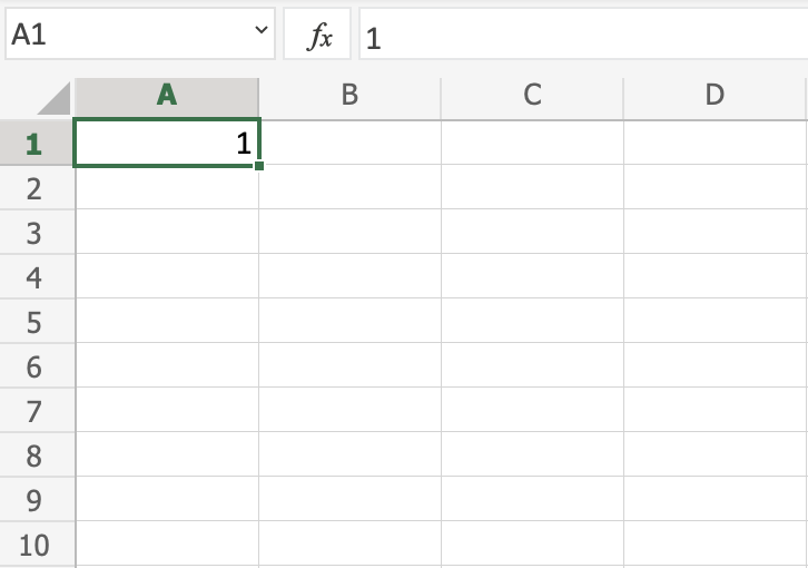
- Enter 1 in cell A1.
- Enter 2 in cell A2.
- Select both the cells and drag it down using the fill handle.
Sometimes it may get a bit irritating to drag the fill handle to the last cell which can be many folds below the current cell.
In this tutorial, I’ll show you a faster way to fill numbers in cells without any dragging.
Quickly Fill Numbers in Cells without Dragging
Here are the steps:
- Enter 1 in cell A1.
- Go to Home –> Editing –> Fill –> Series.

- In the Series dialogue box, make the following selections:
- Series in: Columns
- Type: Linear
- Step Value: 1
- Stop Value: 1000

- Click OK.

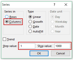
This will fill the cell A1:A1000 with the numbers 1 to 1000.
Notes:
- If you want to fill the numbers in the row instead of the column, select ‘Rows’ in the ‘Series in’ options.
- If you want to start from a number other than 1, fill that number in cell A1. Also, you can choose a different step. For example, select 2 for getting all numbers with a difference of 2.
You May Also Like the Following Excel Tutorials:
- How to Quickly Select Blank Cells in Excel.
- How to Use Format Painter in Excel.
- 7 Quick & Easy Ways to Number Rows in Excel.
- How to Apply Formula to the Entire Column in Excel
- Fill Down Blank Cells Until the Next Value in Excel (Formula, VBA, Power Query)
You can avoid the autofill feature completely with array formulas. Just enter the formula like normal but append :column at the end of each cell reference and then press Ctrl+Shift+Enter. The formula will then be applied immediately to all cells in the column without dragging anything
Edit:
Newer Excel versions will automatically use array formulas to fill down when there’s a new data row
Beginning with the September 2018 update for Office 365, any formula that can return multiple results will automatically spill them either down, or across into neighboring cells. This change in behavior is also accompanied by several new dynamic array functions. Dynamic array formulas, whether they’re using existing functions or the dynamic array functions, only need to be input into a single cell, then confirmed by pressing Enter. Earlier, legacy array formulas require first selecting the entire output range, then confirming the formula with Ctrl+Shift+Enter. They’re commonly referred to as CSE formulas.
Guidelines and examples of array formulas
If you’re on an older version of Excel or want to know more about array formulas then continue reading
For example putting =B3:B + 2*C3:C in D3 and Ctrl+Shift+Enter is equivalent to typing =B3 + 2*C3 and dragging all the way down in a table starting from row 3
That’s fast to type, but has a disadvantage that unused cells at the end (outside the current table) are still calculated and show 0. There’s an easy way to hide the 0s. However the even better way is to limit the calculation to the last column of the table. Knowing that in an array formula you can use X3:X101 to apply to only cells from X3 to X101 we can use INDIRECT function to achieve the same effect
- Enter
=LOOKUP(2, 1/(A:A <> ""), A:A)in some cell outside the table to find the last non-blank cell in the table and name itLastRow. Alternatively use=COUNTA(A3:A) + 2when the table’s first row is 3 - Then instead of
B3:Buse=INDIRECT("B3:B" & LastRow)
For example if you want cells in column D to contain the products of cells in B and C, and column E contains sums of B and C, instead of using D3 = B3*C3 and E3 = B3 + C3 and drag down you just put the below formulas in D3 and E3 respectively and press Ctrl+Shift+Enter
=INDIRECT("B3:B" & LastRow) * INDIRECT("C3:C" & LastRow)
=INDIRECT("B3:B" & LastRow) + INDIRECT("C3:C" & LastRow)
From now on every time you add data to a new row, the table will be automatically updated
Array formula is very fast since the data access pattern is already known. Now instead of doing 100001 different calculations separately, they can be vectorized and done in parallel, utilizing multiple cores and SIMD unit in the CPU. It also has the below advantages:
- Consistency: If you click any of the cells from E2 downward, you see the same formula. That consistency can help ensure greater accuracy.
- Safety: You cannot overwrite a component of a multi-cell array formula. For example, click cell E3 and press Delete. You have to either select the entire range of cells (E2 through E11) and change the formula for the entire array, or leave the array as is. As an added safety measure, you have to press Ctrl+Shift+Enter to confirm the change to the formula.
- Smaller file sizes: You can often use a single array formula instead of several intermediate formulas. For example, the workbook uses one array formula to calculate the results in column E. If you had used standard formulas (such as
=C2*D2,C3*D3,C4*D4…), you would have used 11 different formulas to calculate the same results.Guidelines and examples of array formulas
For more information read
- Create an array formula
Bottom Line: In this post we look at 3 ways to copy down values in blank cells in a column. The techniques include using a formula, Power Query, and a VBA macro.
Skill Level: Intermediate
Watch the Tutorial
Download the Excel Files
You can download both the BEGIN and FINAL files if you want to follow along and practice.
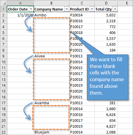
Filling Down Blank Cells
Excel makes it easy to fill down, or copy down, a value into the cells below. You can simply double-click or drag down the fill handle for the cell that you want copied, to populate the cells below it with the same value.
But is there an easy way to replicate that process hundreds of times for reports that have large amounts of data?
In this post we’ll look at three ways to automate this process with: a simple formula, Power Query, and a VBA macro.
1. Filling Down Using a Formula
The first way to solve this problem is by using a very simple formula in all of the blank cells that references the cell above. Here are the steps.
Step 1: Select the Blank Cells
In order to select the blank cells in a column and fill them with a formula, we start by selecting all of the cells (including the populated cells). There are many ways to do this, including holding the Shift key down while you navigate to the bottom of your column, or if your data is in an Excel Table, using the keyboard shortcut Ctrl+Space.
Checkout my posts on 7 Keyboard Shortcuts for Selecting Cells and Ranges in Excel and 5 Keyboard Shortcuts for Rows and Columns in Excel to learn more.
With all of those cells selected, we can pare down our selection to include only the blank cells. This is done by using the Go To Special window from the Find & Select menu on the Home tab of the ribbon.
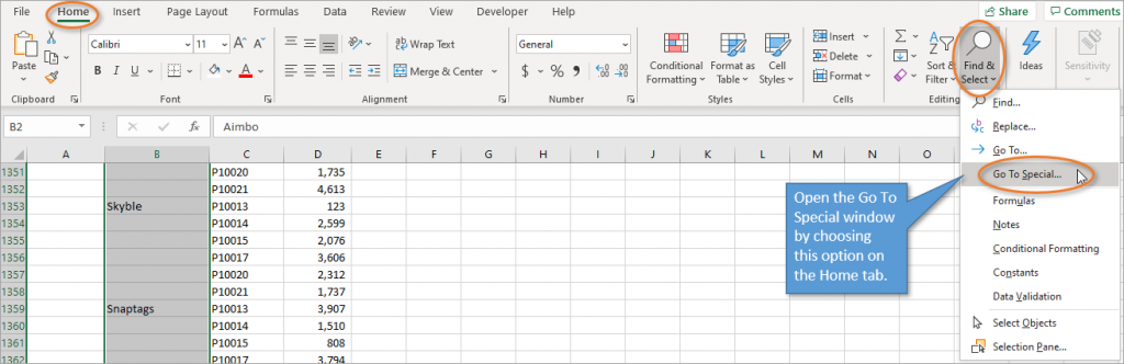
An alternative is to open the Go To window using F5 or Ctrl+G. Then press the Special button for the Go To Special window.
Once the Go To Special window is open, you can choose the option that says Blanks. This will select only the blank cells from the current selection.
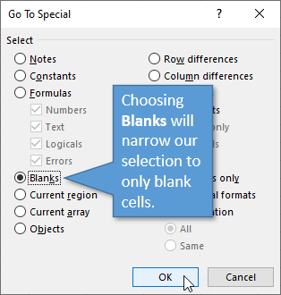
When you hit OK, you’ll notice that the cells that have values in them are no longer selected.
Step 2: Write the Formula
From here you can start typing the formula, which is very simple. Type the equals sign (=) and then reference the cell above (in the case of our example, B2). That’s all you need for the formula!
Step 3: Ctrl+Enter the Formula
After writing the formula, don’t just hit Enter. Instead, use Ctrl+Enter to fill all of the selected cells with the same formula. Hold the Ctrl key, then hit Enter.
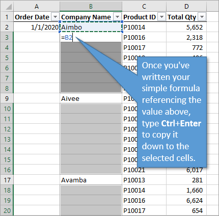
Because your formula reference is relative (B2), not absolute ($B$2), each cell will simply copy the value for the cell directly above it.
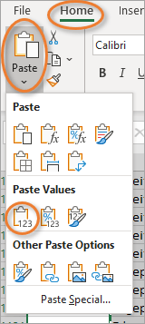
Step 4: Copy & Paste Values
It is a good idea to now copy the entire data column and then paste over it using the Paste Values option so that the data is hard coded. Then, if you do any sorting, the data will not change. You can find the Paste Values option on the Home tab in the Paste drop-down menu:
There are other ways to paste values, including the right-click menu or using keyboard shortcuts. These posts explain those options:
Paste Values with the Right-click & Drag Mouse Shortcut
5 Keyboard Shortcuts to Paste Values in Excel
2. Filling Down Using Power Query
For this option, your data should be in Excel Table format. From anywhere inside the table, you can select the Data or Power Query tab, and then select From Table/Range. You can also create a query that connects to a different data source like a database or the web.
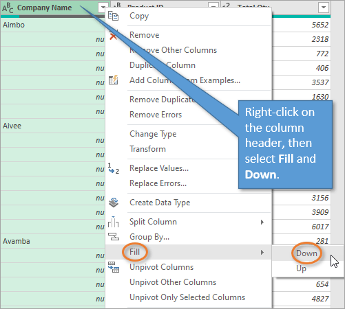
This opens up the Power Query Editor. In Power Query, the blank cells are labeled as null in each cell.
To fill down, just right-click on the column header and select Fill and then Down.
Power Query will fill down each section of blank cells in the column with the value from the cell above it.
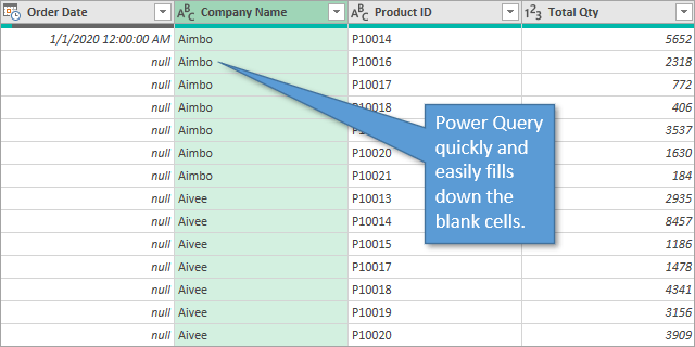
When you click on Close & Load, a new sheet will be added to the workbook with these changes.
This process of filling down can be done for multiple columns simultaneously by first selecting multiple columns with Ctrl or Shift, then performing the Fill > Down operation.
If Power Query is somewhat new to you, I invite you to check out this post: Power Query Overview: An Introduction to Excel’s Most Powerful Data Tool.
Free Webinar on Power Query, VBA, & More
I also have a free webinar running right now that covers an introduction to Power Query and the other Excel tools like Power Pivot, Power BI, Macros & VBA, pivot tables, and more.

Click here to register for the webinar
3. Filling Down Using a Macro
To fill down using a macro, start by opening the VB Editor. You can do this by going to the Developer tab and clicking on the Visual Basic button or by using the keyboard shortcut Alt+F11. Insert a new code module, and then write your macro.
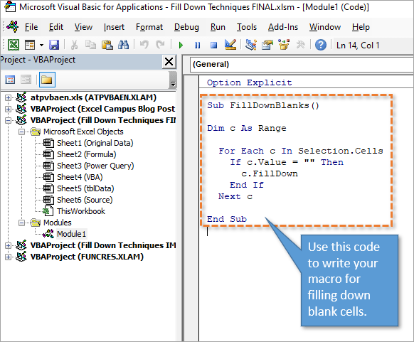
This macro loops through all of the cells in the selected range and performs the FillDown method if the cell is blank. The FillDown method copies the value from the cell above.
If this is a macro that you could use frequently, you might want to consider adding this macro to your personal Macro Workbook and creating a customized button for it. That’s what I’ve done and it looks like this on my Ribbon.
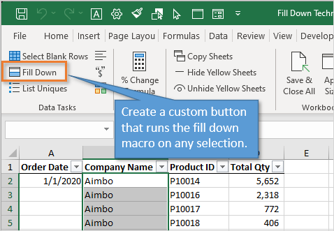
For instruction on how to create a Personal Macro Workbook and custom Ribbon buttons, check out this tutorial: How to Create a Personal Macro Workbook (Video Series).
Pros and Cons
So which of these three methods are right for you? Consider these things:
- The formula method is simple and easy to implement. It can be done without any knowledge of Power Query or VBA. However, it’s not as quick as a one-click button solution.
- Power Query requires source data that outputs into a separate worksheet, so it’s more of a process than simply filling down blank cells. If you are already data cleansing on a regular basis for other things, adding this to your existing process might make more sense.
- Once the initial macro is set up, VBA is a quick solution that’s easy to use—just click a button. However, there is a big disadvantage of this method. You aren’t able to undo your action once that button has been pushed, so you would have to be sure to save a backup copy beforehand if that is a concern for you.
Conclusion
There are three different methods for a very common Excel task. Did I miss any? Please leave a comment below if you have another way to go about it, or have any questions. Thanks! 🙂
Filling
Filling makes your life easier and is used to fill ranges with values, so that you do not have to type manual entries.
Filling can be used for:
- Copying
- Sequences
- Dates
- Functions (*)
For now, do not think of functions. We will cover that in a later chapter.
How To Fill
Filling is done by selecting a cell, clicking the fill icon and selecting the range using drag and mark while holding the left mouse button down.
The fill icon is found in the button right corner of the cell and has the icon of a small square. Once you hover over it your mouse pointer will change its icon to a thin cross.
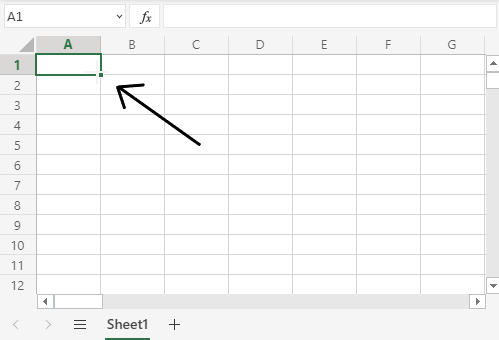
Click the fill icon and hold down the left mouse button, drag and mark the range that you want to cover.
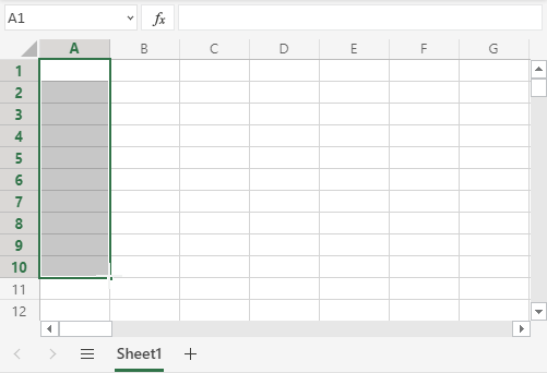
In this example, cell A1 was selected and the range A1:A10 was marked.
Now that we have learned how to fill. Let’s look into how to copy with the fill function.
Fill Copies
Filling can be used for copying. It can be used for both numbers and words.
Let’s have a look at numbers first.
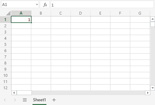
In this example we have typed the value A1(1):
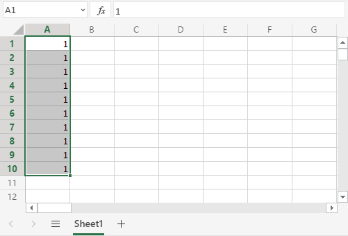
Filling the range A1:A10 creates ten copies of
1:
The same principle goes for text.
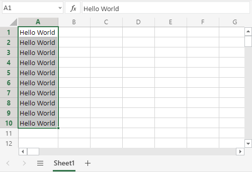
In this example we have typed A1(Hello World).
Filling the range A1:A10 creates ten copies of «Hello World»:
Now you have learned how to fill and to use it for copying both numbers and words. Let’s have a look at sequences.
Fill Sequences
Filling can be used to create sequences. A sequence is an order or a pattern. We can use the filling function to continue the order that has been set.
Sequences can for example be used on numbers and dates.
Let’s start with learning how to count from 1 to 10.
This is different from the last example because this time we do not want to copy, but to count from 1 to 10.
Start with typing A1(1):
First we will show an example which does not work, then we will do a working one. Ready?
Lets type the value (1) into the cell A2, which is what we have in A1. Now we have the same values in both A1 and A2.
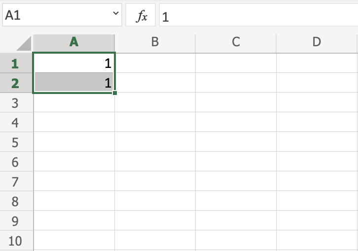
Let’s use the fill function from A1:A10 to see what happens. Remember to mark both values before you fill the range.
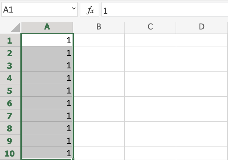
What happened is that we got the same values as we did with copying. This is because the fill function assumes that we want to create copies as we had two of the same values in both the cells A1(1) and A2(1).
Change the value of A2(1) to A2(2). We now have two different values in the cells A1(1) and A2(2). Now, fill A1:A10
again. Remember to mark both the values (holding down shift) before you fill the
range:
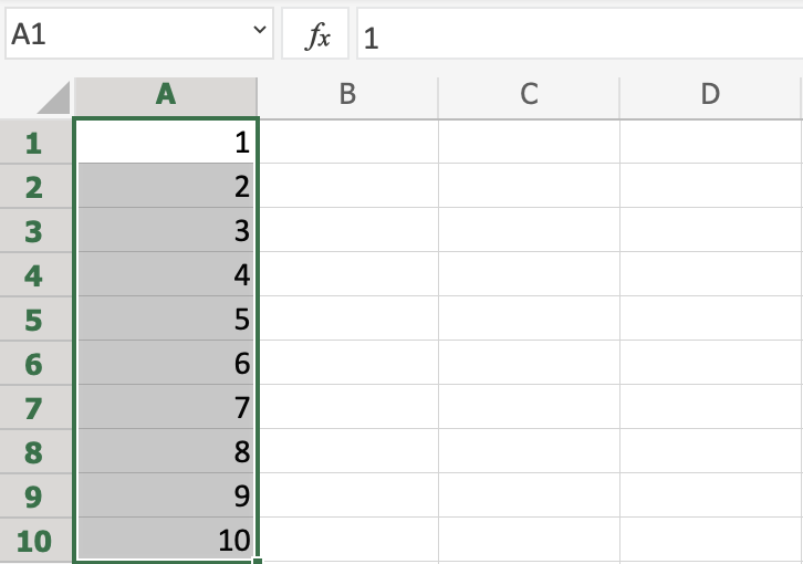
Congratulations! You have now counted from 1 to 10.
The fill function understands the pattern typed in the cells and continues it for us.
That is why it created copies when we had entered the value (1) in both cells,
as it saw no pattern. When we entered (1) and (2) in the cells it was able to understand the pattern and that the next cell A3 should be (3).
Let’s create another sequence. Type A1(2) and A2(4):
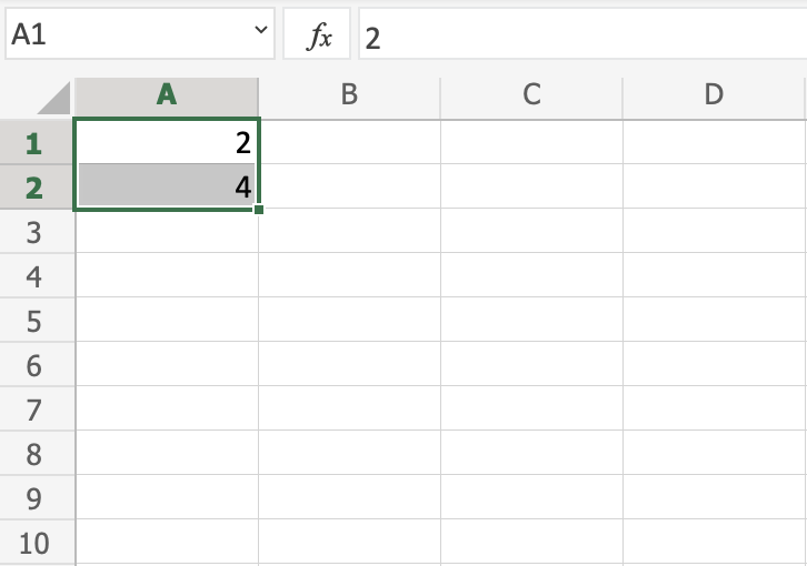
Now, fill A1:A10:
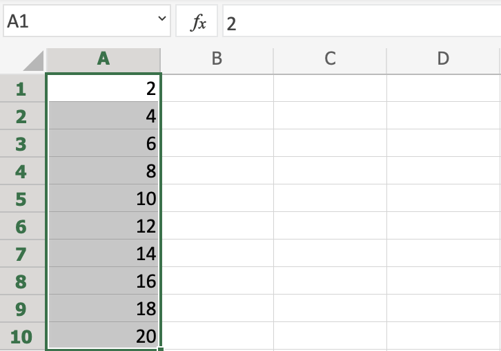
It counts from 2 to 20 in the range A1:A10.
This is because we created an order with A1(2) and A2(4).
Then it fills the next cells, A3(6), A4(8), A5(10) and so on. The fill function understands the pattern and helps us continue it.
Sequence of Dates
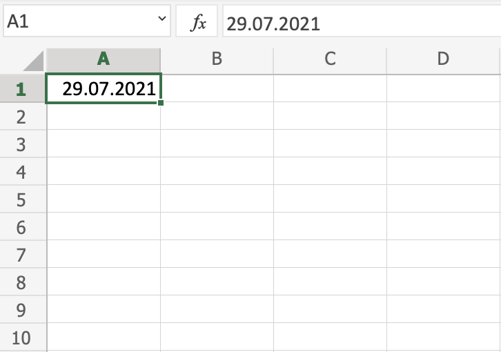
The fill function can also be used to fill dates.
Test it by typing A1(29.07.2021):
And fill the range A1:A10:
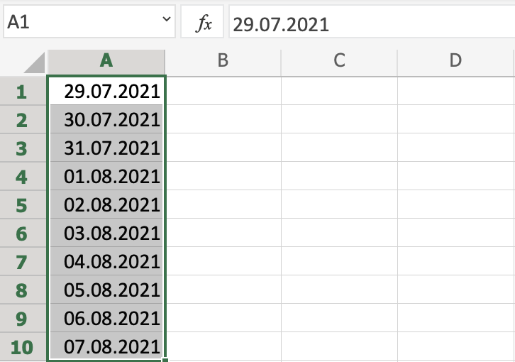
The fill function has filled 10 days from A1(29.07.2021) to A10(07.08.2021).
Note that it switched from July to August in cell A4. It knows the calendar and will count real dates.
Combining Words and Letters
Words and letters can also be combined.
Type A1(Hello 1) and A2(Hello 2):
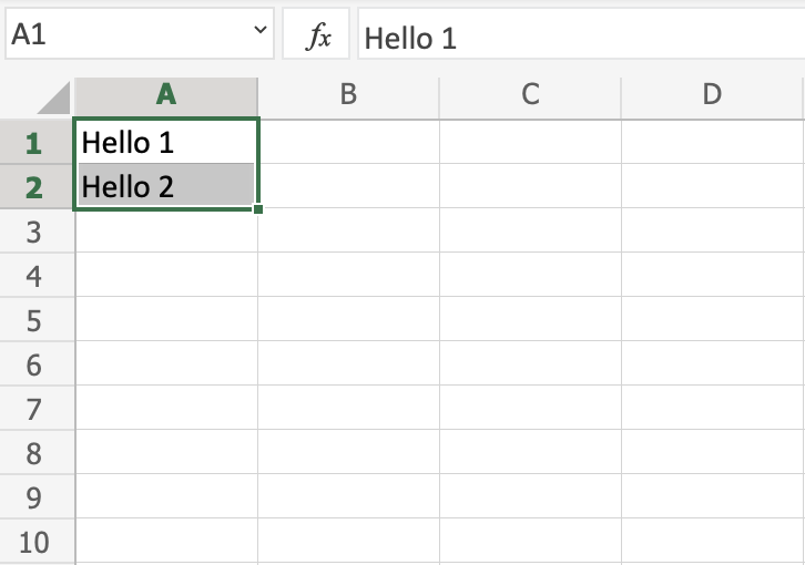
Next, fill A1:A10 to see what happens:
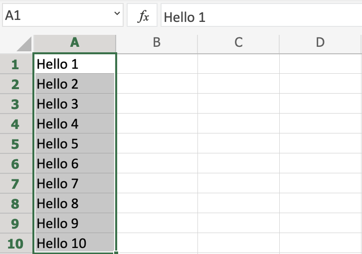
The result is that it counts from A1(Hello 1) to A10(Hello 10). Only the numbers have changed.
It recognised the pattern of the numbers and continued it for us. Words and numbers can be combined, as long as you use a recognizable pattern for the numbers.
Test Yourself With Exercises
Excel is really cool when it comes to automatically filling in cells in columns or rows with weekdays, months etc etc…so when you type in the first couple of items in the list, then drag the fill handle, Excel then does the hard work for you.
So, are you resticted to having the in built lists that Microsoft has so kindly set for us?.
No, you aren’t.
You can add in your own custom lists- anything you want, so whether it is a list of products, class members or employees, you can pre program these into an Excel custom list, type in the first value in your list, drag the fill handle as normal and your customized list will be filled in for you.
There are actually two quick ways to add in your own custom list. Let’s work through an example
- File Tab
- Options- the options dialog box will appear
- Advanced Tab- Advanced options appears in the right hand pane image
- Click Edit Custom Lists in the General Section- the Custom Lists dialog box will appear
- Click inside List Entries and type in your list items in the order you want- in this example it is fruit products

- Click Ok twice to save your new Custom List
So- that was the first method to use your own list.
As an alternative if you already have a list that you use regularly-
- Open your workbook or or navigate to the worksheet that contains your list
- Use the data selection to specify the range of cells
- Hit Import
- Hit Ok

Want More Excel Tips?
1. The LEN function in Excel
2. Awesome Excel shortcut- drawing borders

Create a blank template containing only the column headers.
In the first cell of the row below the column headers, let’s say A2, enter the formula =A1. This will make A2 have the same value as the cell above it, unless it’s overridden. Select this cell (A2), copy, and paste to all of the columns that you want to have this repeating feature, for more than enough rows. (That is, if you want the feature to work in the first three columns, and if you anticipate never needing more than 100 rows, paste to the range A2 — C101.)
Now, make a copy of the blank template, and enter your data into the appropriate cells. Each value will be copied downward until the next manually-entered value. If you need to do this again, start over with a new copy of your blank template.
If you enter a value but then want to delete it, copy one of the cells that’s still automatically copied from above and paste it into the cell you want to delete. That will revert it back to being automatically filled in from above.