
You can add shading to cells by filling them with solid colors or specific patterns. If you have trouble printing the cell shading that you applied in color, verify that print options are set correctly.
Fill cells with solid colors
-
Select the cells that you want to apply shading to or remove shading from. For more information on selecting cells in a worksheet, see Select cells, ranges, rows, or columns on a worksheet.
-
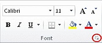
On the Home tab, in the Font group, do one of the following:

-
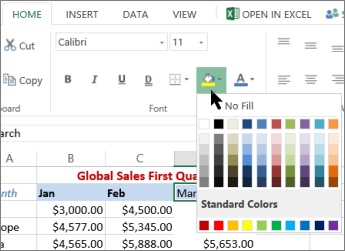
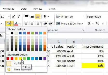
To fill cells with a solid color, click the arrow next to Fill Color
, and then under Theme Colors or Standard Colors, click the color that you want. -
To fill cells with a custom color, click the arrow next to Fill Color
, click More Colors, and then in the Colors dialog box select the color that you want. -
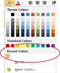
To apply the most recently selected color, click Fill Color
.Note: Microsoft Excel saves your 10 most recently selected custom colors. To quickly apply one of these colors, click the arrow next to Fill Color
, and then click the color that you want under Recent Colors.
-
Tip: If you want to use a different background color for the whole worksheet, click the Select All button before you click the color that you want to use. This will hide the gridlines, but you can improve worksheet readability by displaying cell borders around all cells.

Fill cells with patterns
-
Select the cells that you want to fill a pattern with. For more information on selecting cells in a worksheet, see Select cells, ranges, rows, or columns on a worksheet.
-
On the Home tab, in the Font group, click the Format Cells dialog box launcher.
Keyboard shortcut You can also press CTRL+SHIFT+F.
-
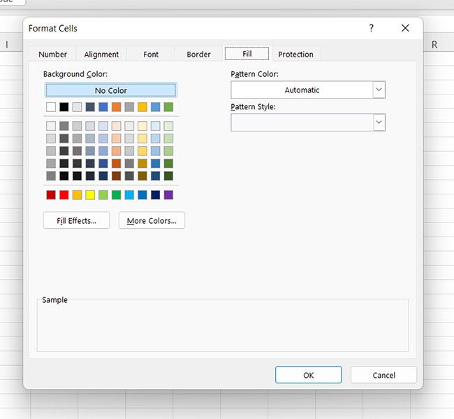
In the Format Cells dialog box, on the Fill tab, under Background Color, click the background color that you want to use.
-
Do one of the following:
-
To use a pattern with two colors, click another color in the Pattern Color box, and then click a pattern style in the Pattern Style box.
-
To use a pattern with special effects, click Fill Effects, and then click the options that you want on the Gradient tab.
-
Verify print options to print cell shading in color
If print options are set to Black and white or Draft quality — either on purpose, or because the workbook contains large or complex worksheets and charts that caused draft mode to be turned on automatically — cell shading cannot print in color.
-
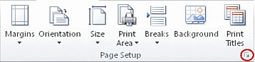
On the Page Layout tab, in the Page Setup group, click the Page Setup dialog box launcher.
-
On the Sheet tab, under Print, make sure that the Black and white and Draft quality check boxes are cleared.
Note: If you do not see colors in the worksheet, it may be that you are working in high contrast mode. If you do not see colors when you preview before you print, it may be that you do not have a color printer selected.
Remove cell shading
-
Select the cells that contain a fill color or fill pattern. For more information on selecting cells in a worksheet, see Select cells, ranges, rows, or columns on a worksheet
-
On the Home tab, in the Font group, click the arrow next to Fill Color, and then click No Fill.
Set a default fill color for all cells in a worksheet
In Excel, you cannot change the default fill color for a worksheet. By default, all cells in a workbook contain no fill. However, if you frequently create workbooks that contain worksheets with cells that all have a specific fill color, you can create an Excel template. For example, if you frequently create workbooks where all the cells are green, you can create a template to simplify this task. To do this, follow these steps:
-
Create a new, blank worksheet.
-
Click the Select All button, to select the whole worksheet.
-
On the Home tab, in the Font group, click the arrow next to Fill Color
, and then select the color that you want. Tip When you change the fill colors of the cells on a worksheet, the gridlines can become difficult to see. To make the gridlines stand out on the screen, you can experiment with border and line styles. These settings are located on the Home tab, in the Font group. To apply borders to your worksheet, select the entire worksheet, click the arrow next to Borders
, and then click All Borders. -
On the File tab, click Save As.
-
In the File name box, type the name that you want to use for the template.
-
In the Save as type box, click Excel Template, click Save, and then close the worksheet.
The template is automatically placed in the Templates folder to make sure that it will be available when you want to use it to create a new workbook.
-
To open a new workbook based on the template, do the following:
-
On the File tab, click New.
-
Under Available Templates, click My templates.
-
In the New dialog box, under Personal Templates, click the template that you just created.
-
 , and then click All Borders.
Top of Page
Learn how to apply Excel fill color shortcut to change the background or shading colors of a cell using various methods.
In this guide, all demonstrated fill color shortcuts are for Excel for Windows versions 2010, 2013, 2016, 2019, and Office365.
If you are looking for keyboard shortcuts to fill a cell quickly, you are at the right place. In this article, we’ll show you the best practices and workarounds.
Table of content:
- How to use the fill color shortcut in Excel
- Apply the Alt, H, H shortcut
- The fastest way: Fill Color Shortcuts Add-in in Excel
- Add Fill Color Menu to Quick Access Toolbar
The fact is that there is no built-in keyboard shortcut in Excel that fills color to a cell. Luckily, Excel offers some workarounds to perform this task.
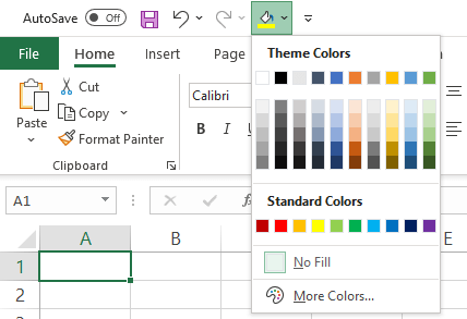
Apply the Alt, H, H shortcut to open the Fill color menu
To open the Fill Color menu, use the Alt, H, H shortcut, and Excel shows the color palette dialog. You can view the color palettes, the theme colors, and the standard colors.
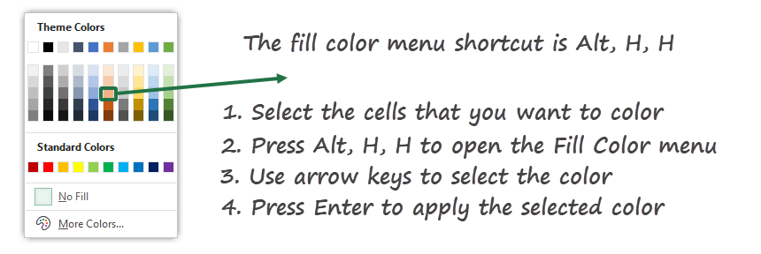
Steps to apply a fill color shortcut:
- Select the cells that you want to color
- Press Alt, H, H top open the Fill color menu
- Use the arrow keys to move on the color grid
- Select the color that you want to apply
- Press Enter to fill color to the selected cell or range
Shortcut to use no fill: Alt, H, H, N
Shortcut to show more colors on the palette: Alt, H, H, M
This way is a bit faster than the default method (Clicking the Home Tab and using the Colors drop-down menu)
Fill Color Shortcuts Add-in in Excel
If you are familiar with VBA, we have a piece of good news. VBA makes life easier. I wrote a tiny custom Excel add-in that allows you to assign custom keyboard shortcuts for all purposes.
This guide will demonstrate the fastest way to apply a command using a user-defined shortcut key.
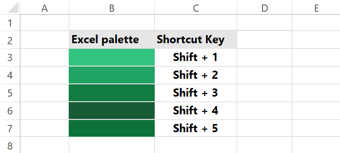
In the example, you want to use the Excel green color palette for your reports. The Application.Onkey method help to assign a fill color shortcut key to color.
Press Alt + F11 to open the VBA editor window and copy the code to ThisWorkBook:
Option Explicit
Private WithEvents appEvents As Application
Private Sub Workbook_Open()
Set appEvents = Application
Application.OnKey "+1", "Fill_Green1"
Application.OnKey "+2", "Fill_Green2"
Application.OnKey "+3", "Fill_Green3"
Application.OnKey "+4", "Fill_Green4"
Application.OnKey "+5", "Fill_Green5"
End Sub
Create a new module and add the following code:
Sub Fill_Green1()
Selection.Interior.Color = RGB(51, 196, 129)
End Sub
Sub Fill_Green2()
Selection.Interior.Color = RGB(33, 163, 102)
End Sub
Sub Fill_Green3()
Selection.Interior.Color = RGB(16, 124, 65)
End Sub
Sub Fill_Green4()
Selection.Interior.Color = RGB(24, 92, 55)
End Sub
Sub Fill_Green5()
Selection.Interior.Color = RGB(13, 114, 57)
End Sub
The new shortcut keys are: Shift +1 to Shift +5
You can download the fill color add-in here. Play with it; replace the code if you want. Also, don’t forget to check this guide on how to install an Excel add-in.
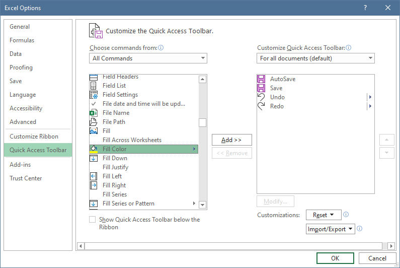
If you don’t want to use keyboard shortcuts, there is a way to pin the Fill Color menu on the Quick Access Toolbar.
- Click File > Options
- Select the Quick Access Toolbar from the list
- Select All commands and choose the Fill color
- Add the command to the QAT, then click OK
Now the menu appears in the QAT. From now on, you can use the method mentioned above to select the fill color.
Steps to using a fill cell color command:
- Add the Fill color menu to the QAT
- Press Alt, 5 (or position number in the QAT) to open the Fill Color dialog
- Use the arrow keys to navigate between colors and select the color
- Press Enter to apply the selected color to the cell or range of cells
This way is an excellent alternative to the Alt, H, H fill color shortcut. We recommend you place the most frequently used commands in the QAT. It is not necessary to switch between Excel tabs to reach the fill color command.
Repeat the last action using F4 Key or Alt+Enter
Sometimes it can be useful if you can repeat the last action. In Excel, the shortcut key for this purpose is F4.
In the example, we have used the Alt, H, H fill color shortcut to apply a green background to cell B3. Next, move the cursor to cell B4, then press F4.
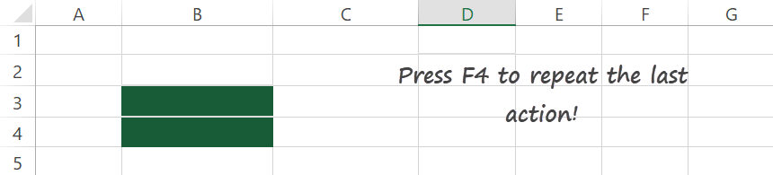
Excel will repeat the last action and will use a green background for cell B3. So easy!
Copy and Paste formatting using shortcuts
Last but not least, you can use the copy formatting command to apply a fill color to a cell.
Steps to apply the Paste Formatting Button on the QAT:
- Add the Paste Formatting button to the QAT
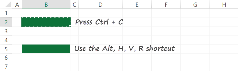
- Copy the cell (Ctrl + C) that contains the formatting style
- Select the destination cell or the range of cells
- Press Alt+5 (or the current position number of the QAT button) to apply the formatting
Tip: You can use one of a paste special shortcut keys to speed up the task. After pressing Ctrl + C, select the target cell or range and use the Alt, H, V, R Paste Format keyboard shortcut.
Final thoughts
Today we have introduced some tricks to apply the fill color shortcut in Excel. Pick your favorite way! Also, we recommend using our small, flexible add-in. Stay tuned.
Additional resources:
- Excel Shortcuts – The Ultimate Guide
Filling a background color in a cell or range of cells is a common task that most of Excel users have to do on a daily basis.
While it’s quite easy to fill color in a cell in Excel (using the inbuilt option in the ribbon), it’s not the fastest way to do it.
And if this is something you have to do multiple times in a day, knowing faster ways to fill color in a cell would make you more efficient and also save time.
And needless to say, you can always use the shortcuts and tricks I cover in this tutorial to impress your boss and colleagues.
Regular Way to Fill Color in Cells
Before I show you some shortcut ways to fill color in Excel, let me quickly show you the regular way of doing it:
- Select the cell or range of cells in which you want to fill the color
- Click the ‘Home’ tab

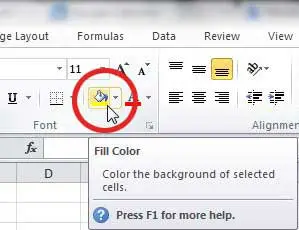
- In the Font group, click on the ‘Fill Color’ icon
- Click on the color that you want to fill in the selected cell

If you don’t find the color you want to fill in the options that show up in Step 3, you can click on the ‘More Colors’ options.
This will open the colors dialog box where you get more colors as well as the option to specify the hex color code or the RGB code

Fun Fact: There are approximately 16.6 million different colors you can use in Excel
Shortcuts to Fill Color in Cells in Excel
Let’s look at some shortcut ways you can use to fill color in cells in Excel.
Keyboard Shortcut to Fill Color in Cells
Let’s start with a keyboard shortcut that will quickly allow you to open the options that show all the colors that you can fill in a cell (all the selected range of cells).
ALT + H + H
To use this keyboard shortcut, you first need to select the cell or the range of cells in which you want to fill the color and then hit these keys in succession (ALT then H, and then H).
The above keyboard shortcut would open the Fill Color panel that shows you all the colors, where you can use the arrow keys to navigate to the color you want to fill and then hit the Enter key.
While this keyboard shortcut may seem faster than using your mouse to click on the Home tab and then click on the color panel and then select the color, one major drawback of this method is that you cannot select the color you need with this keyboard shortcut. You need to use the arrow keys to navigate to the color you want, which makes this keyboard shortcut slow to use
Pros of this shortcut
- Faster than using the mouse (once you get used to it)
- Allows you to not switch from keyboard to mouse
Cons of this shortcut
- Doesn’t allow selecting a color and you need to navigate using the arrow keys
- Slower than expected
- Hard to remember
Pro Tip: If you want to quickly remove the color from a cell or range of cells, you can use the keyboard shortcut ALT + H + H + N
Adding Fill Color Option to the Quick Access Toolbar (QAT)
You can also add the Fill Color icon in the Quick Access Toolbar so that you always have access to it with a single click.
So, instead of going to the Home tab and then locating the Fill Color icon, you can get the same option with a single click.
Below are the steps to add the fill color icon in the Quick Access Toolbar:
- In the Quick Access Toolbar click on the ‘Customize the Quick Access Toolbar’ icon

- In the options that show up, click on ‘More Commands’

- In the ‘Excel Options’ dialog box that opens up, select the ‘Fill Color’ icon option

- Click on the Add button

- Click OK
The above steps would add the fill color icon in the QAT.
To use this, just click on the ‘Fill Color’ icon in the QAT and it’ll show you the palette of colors that you can choose from.
One big benefit of adding icons in the Quick Access Toolbar is that you can also use these icons with a simple keyboard shortcut:
ALT + Number (which is the position of the icon in the QAT)
In our example, since the Fill Color icon is the second option in the QAT, I can use the keyboard shortcut ALT + 2 (where I need to hold the ALT key and then press the 2 key)
As you can see, this keyboard shortcut is a lot better than the regular keyboard shortcut of the fill color icon ALT + H + H
Pros
- You always have access to the Fill Color option with a single click
- The keyboard shortcut for icons in the QAT is usually shorter
Cons
- You need to add the Fill color icon in the QAT first (one-time effort)
- If you use the mouse to access it, it only saves you one click (so not significantly better than using the option in the ribbon)
Using F4 to Repeat Fill Color Operation
This is not really a direct keyboard shortcut to fill color in any cell or range of cells, however, if you have already used one of the above options to fill color in a cell or range, you can repeat the same action by using the F4 key.
Here is how you can use the F4 key to fill color in Excel:
- Select a cell in which you want to fill the color
- Use the keyboard shortcut or the Fill Color icon in the ribbon to fill the color in the selected cell
- Now select any other cell or range of cells that you want to fill with the same color
- Hit the F4 key
When you use the F4 key in Step 4, it repeats the same action that has been done just before using it.
In our example, since we first filled a cell with a specific color, and then use the F4 key, it repeated the same action.
You can continue to use the F4 key to fill color in multiple cells/ranges as long as you don’t do anything else.
You can even use this across worksheets and other open workbooks
Pros:
- Huge timesaver as you can do the action once and repeat it as many times as you want
- Works across other worksheets as well as other open workbooks
Cons:
- Since it’s dependent on the last action, as soon as you do anything else, you won’t be able to use this keyboard shortcut to fill the color
[Advanced] Creating Your Own Shortcut to Fill Color Using VBA
If there is some specific color that you often need to fill in Excel, you can create your own VBA code and install that as an add-in.
Once you do that, you will be able to use simple keyboard shortcuts (that you yourself assign in the VBA code) to quickly fill color in the selected cells.
Below are the detailed steps to create an add-in using VBA code that will allow you to use shortcuts to fill color in the selected cells:
- Open a new Excel workbook
- Click the Developer tab and then click on the Visual Basic icon. this will open the VBA editor. If you do not see the Developer tab, you can use the keyboard shortcut ALT + F11 (or read this guide on how to get the developer tab in the ribbon)
- In Project Explorer, double-click on the ‘ThisWorkbook’ object. If you don’t see Project Explorer, click on the ‘View’ option in the menu and then click on ‘Project Explorer’
- Copy and paste the below code into the ThisWorkbook code window
Private Sub Workbook_Open()
Set AppEvents = Application
Application.OnKey "+1", "Fill_Red"
Application.OnKey "+2", "Fill_Blue"
Application.OnKey "+3", "Fill_Green"
End Sub

- Click the Insert option in the menu and click on ‘Module’. This will insert a new module for this workbook

- Copy and paste the below code in the module code window
Sub Fill_Red()
Selection.Interior.Color = RGB(255, 0, 0)
End Sub

Sub Fill_Blue()
Selection.Interior.Color = RGB(0, 0, 255)
End Sub

Sub Fill_Green()
Selection.Interior.Color = RGB(0, 255, 0)
End Sub

- Close the VB editor
- Click the File tab and then click on Save As

- Click on the Browse option and select the location where you want to save the add-in

- Give the Add-in a name

- In the ‘Save as type’ drop-down, select the Excel add-in (.XLAM) option

- Click on Save
With the above steps, we have our add-in that we can install in any Excel workbook so that the VBA code would be available in all the workbooks on our system.
Below are the steps to add this add-in into an excel workbook:
- Open a new Excel workbook (you can also use any existing workbook that is already open)
- Click the Developer tab
- In the Add-ins group, click on Excel Add-ins

- In the Add-ins dialog box, click the ‘Browse’ button

- Locate and select the add-in that we have already created and saved

- Click Ok
- Click OK in the Add-ins dialog box (make sure the add-in you added is checked)

The above steps have added the add-in we created to the Excel workbook. And going forward, this add-in would be available in all the Excel workbooks that you use on your system (new as well as existing)
Now you can use the below keyboard shortcuts to fill color in selected cells in Excel.
To fill Red color:
Shift + 1
To fill Blue color:
Shift + 2
To fill Green color:
Shift + 3
In this example, I have shown you how to create a couple of keyboard shortcuts that you can use to fill red, blue, or green colors in the selected cells.
You can modify the VBA code to specify your own color and even create more keyboard shortcuts.
Note: You need to keep the add-in file that we created in the same location for the add-in to continue to work. If you delete this file, you won’t be able to use this add-in in any of the Excel files. In case you change the location of the add-in file, you need to install it again.
Pros:
- Easy to use once set-up
- You can create your own shortcuts and use these in any workbook once the add-in is installed
Cons
- The initial setup is long and a bit advanced for beginner Excel users
- Add-ins can sometimes create issues and conflict with existing Excel features or other add-ins
Using Paint Format to Easily Copy and Fill Colors
Excel also allows you to quickly copy the formatting from one cell (or a range of cells) and paste this formatting to other cells.
This can easily be done using the Format Painter tool.
And since the color of the cell is part of the formatting, you can also use this to quickly copy the color of any cell end applied to other cells
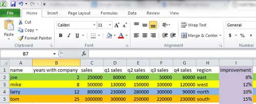
Below I have a data set where I have cell color in some of the headers that contain the month name, I need to fill the same color in the other headers that do not have any color in the cell.

Since I want the same color to be filled to the headers in cells D1, E1, and F1, instead of doing it manually, I can copy the color from the existing colored cell, and then apply it to these non-filled cells.
Below are the steps to fill color using Format Painter:
- Select the cell that already has the color that you want to copy
- Click the Home tab
- In the Clipboard group, click on the Format Painter icon
- Select the cell (or range of cells) on which you want to fill the same color

Pro Tip: If you want to continue to use the format painter to fill color in multiple cells, double-click on the format painter icon in Step 3. When you click on the format painter icon once, you can only use it once, but when you double click on it, it remains active unless you hit the Escape key or use some other option
Remember that the format printer option would copy all the formatting of the source cell and apply it to the destination cell. This could include cell color, border, font color font size, as well as conditional formatting.
One way many advanced Excel users use the Format Painter tool is to copy the conditional formatting rules from one area and apply it to some other area in the worksheet.
In this tutorial, I showed you some shortcut methods you can use to fill color in the cells in Excel. You can use a keyboard shortcut or add the Fill color icon in the Quick Access Toolbar to use it.
And if you need some specific colors to be quickly applied to the selected cells, you can also consider using the VBA method that allows you to create your own keyboard shortcuts. You can create an add-in using the VBA code so that these shortcuts are available in all the Excel files on your system.
I hope you found this excel tutorial useful.
Other Excel articles you may also find helpful:
- Excel Paste Special Shortcuts That Will Save You Tons of Time
- How to Select Entire Column (or Row) in Excel – Shortcut
- How to Indent in Excel (3 Easy Ways + Keyboard Shortcut)
- Copy and Paste Multiple Cells in Excel (Adjacent & Non-Adjacent)
- 200+ Excel Keyboard Shortcuts – 10x Your Productivity
- How to Sum by Color in Excel (Formula & VBA)
- How to Sort By Color in Excel (in less than 10 seconds)
- How to Count Colored Cells in Excel – A Step by Step Tutorial + Video
- How to Edit Cells in Excel? (Shortcuts)
Содержание
- Highlight cells
- Create a cell style to highlight cells
- Use Format Painter to apply a highlight to other cells
- Display specific data in a different font color or format
- Add or change the background color of cells
- Apply a pattern or fill effects
- Remove cell colors, patterns, or fill effects
- Print cell colors, patterns, or fill effects in color
- Remove fill color
- Need more help?
- Best Shortcuts to Fill Color in Excel (Basic & Advanced)
- Regular Way to Fill Color in Cells
- Shortcuts to Fill Color in Cells in Excel
- Keyboard Shortcut to Fill Color in Cells
- Adding Fill Color Option to the Quick Access Toolbar (QAT)
- Using F4 to Repeat Fill Color Operation
- [Advanced] Creating Your Own Shortcut to Fill Color Using VBA
- Using Paint Format to Easily Copy and Fill Colors
Highlight cells
Unlike other Microsoft Office programs, such as Word, Excel does not provide a button that you can use to highlight all or individual portions of data in a cell.
However, you can mimic highlights on a cell in a worksheet by filling the cells with a highlighting color. For a fast way to mimic a highlight, you can create a custom cell style that you can apply to fill cells with a highlighting color. Then, after you apply that cell style to highlight cells, you can quickly copy the highlighting to other cells by using Format Painter.
If you want to make specific data in a cell stand out, you can display that data in a different font color or format.
Create a cell style to highlight cells
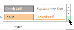
Click Home > New Cell Styles.
If you don’t see Cell Style, click the More  button next to the cell style gallery.
In the Style name box, type an appropriate name for the new cell style.
Tip: For example, type Highlight.
In the Format Cells dialog box, on the Fill tab, select the color that you want to use for the highlight, and then click OK.
Click OK to close the Style dialog box.
The new style will be added under Custom in the cell styles box.
On the worksheet, select the cells or ranges of cells that you want to highlight. How to select cells?
On the Home tab, in the Styles group, click the new custom cell style you created.
Note: Custom cell styles are displayed at the top of the list of cell styles. If you see the cell styles box in the Styles group, and the new cell style is one of the first six cell styles on the list, you can click that cell style directly in the Styles group.
Use Format Painter to apply a highlight to other cells
Select a cell that is formatted with the highlight that you want to use.
On the Home tab, in the Clipboard group, double-click Format Painter  , and then drag the mouse pointer across as many cells or ranges of cells that you want to highlight.
When you’re done, click Format Painter again or press ESC to turn it off.
Display specific data in a different font color or format
In a cell, select the data that you want to display in a different color or format.
How to select data in a cell
To select the contents of a cell
Double-click the cell, and then drag across the contents of the cell that you want to select.
In the formula bar 
Click the cell, and then drag across the contents of the cell that you want to select in the formula bar.
By using the keyboard
Press F2 to edit the cell, use the arrow keys to position the insertion point, and then press SHIFT+ARROW key to select the contents.
On the Home tab, in the Font group, do one of the following:
To change the text color, click the arrow next to Font Color  and then, under Theme Colors or Standard Colors, click the color that you want to use.
To apply the most recently selected text color, click Font Color .
To apply a color other than the available theme colors and standard colors, click More Colors, and then define the color that you want to use on the Standard tab or Custom tab of the Colors dialog box.
To change the format, click Bold  , Italic
  , or Underline
  .
.
Keyboard shortcut You can also press CTRL+B, CTRL+I, or CTRL+U.
Источник
Add or change the background color of cells
You can highlight data in cells by using Fill Color to add or change the background color or pattern of cells. Here’s how:
Select the cells you want to highlight.
To use a different background color for the whole worksheet, click the Select All button. This will hide the gridlines, but you can improve worksheet readability by displaying cell borders around all cells.
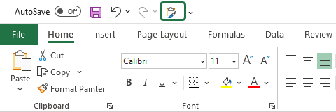
Click Home > the arrow next to Fill Color  , or press Alt+H, H.
Under Theme Colors or Standard Colors, pick the color you want.
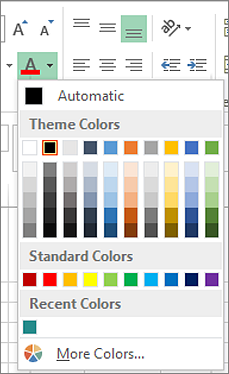
To use a custom color, click More Colors, and then in the Colors dialog box select the color you want.
Tip: To apply the most recently selected color, you can just click Fill Color . You’ll also find up to 10 most recently selected custom colors under Recent Colors.
Apply a pattern or fill effects
When you want something more than a just a solid color fill, try applying a pattern or fill effects.
Select the cell or range of cells you want to format.
Click Home > Format Cells dialog launcher, or press Ctrl+Shift+F.
On the Fill tab, under Background Color, pick the color you want.
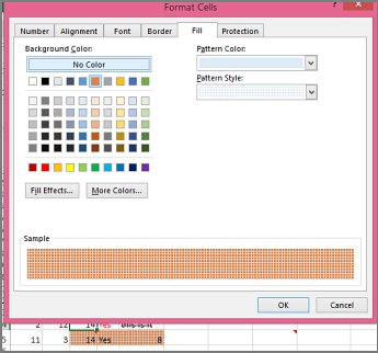
To use a pattern with two colors, pick a color in the Pattern Color box, and then pick a pattern in the Pattern Style box.
To use a pattern with special effects, click Fill Effects, and then pick the options you want.
Tip: In the Sample box, you can preview the background, pattern, and fill effects you selected.
Remove cell colors, patterns, or fill effects
To remove any background colors, patterns, or fill effects from cells, just select the cells. Then click Home > arrow next to Fill Color, and then pick No Fill.
Print cell colors, patterns, or fill effects in color
If print options are set to Black and white or Draft quality — either on purpose, or because the workbook has large or complex worksheets and charts that caused draft mode to be turned on automatically — cells won’t print in color. Here’s how you can fix that:
Click Page Layout > Page Setup dialog box launcher.
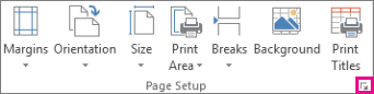
On the Sheet tab, under Print, uncheck the Black and white and Draft quality check boxes.
Note: If you don’t see colors in your worksheet, it may be that you’re working in high contrast mode. If you don’t see colors when you preview before you print, it may be that you don’t have a color printer selected.
If you’d like to highlight text or numbers to make the data more visible, try either changing the font color or add a background color to the cell or range of cells like this:

Select the cell or range of cells for which you want to add a fill color.
On the Home tab, click Fill Color, and pick the color you want.
Note: Pattern fill effects for background colors are not available for Excel for the web. If you apply any from Excel on your desktop, it won’t appear in the browser.
Remove fill color
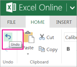
If you decide that you don’t want the fill color immediately after you added it, just click Undo .
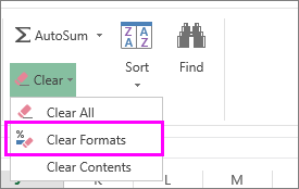
To remove the fill color at a later time, select the cell or cell range you want to change, and click Clear > Clear Formats.
Need more help?
You can always ask an expert in the Excel Tech Community or get support in the Answers community.
Источник
Best Shortcuts to Fill Color in Excel (Basic & Advanced)
Filling a background color in a cell or range of cells is a common task that most of Excel users have to do on a daily basis.
While it’s quite easy to fill color in a cell in Excel (using the inbuilt option in the ribbon), it’s not the fastest way to do it.
And if this is something you have to do multiple times in a day, knowing faster ways to fill color in a cell would make you more efficient and also save time.
And needless to say, you can always use the shortcuts and tricks I cover in this tutorial to impress your boss and colleagues.
This Tutorial Covers:
Regular Way to Fill Color in Cells
Before I show you some shortcut ways to fill color in Excel, let me quickly show you the regular way of doing it:
- Select the cell or range of cells in which you want to fill the color
- Click the ‘Home’ tab
- In the Font group, click on the ‘Fill Color’ icon
- Click on the color that you want to fill in the selected cell
If you don’t find the color you want to fill in the options that show up in Step 3, you can click on the ‘More Colors’ options.
This will open the colors dialog box where you get more colors as well as the option to specify the hex color code or the RGB code
Fun Fact: There are approximately 16.6 million different colors you can use in Excel
Shortcuts to Fill Color in Cells in Excel
Let’s look at some shortcut ways you can use to fill color in cells in Excel.
Keyboard Shortcut to Fill Color in Cells
Let’s start with a keyboard shortcut that will quickly allow you to open the options that show all the colors that you can fill in a cell (all the selected range of cells).
To use this keyboard shortcut, you first need to select the cell or the range of cells in which you want to fill the color and then hit these keys in succession (ALT then H, and then H).
The above keyboard shortcut would open the Fill Color panel that shows you all the colors, where you can use the arrow keys to navigate to the color you want to fill and then hit the Enter key.
While this keyboard shortcut may seem faster than using your mouse to click on the Home tab and then click on the color panel and then select the color, one major drawback of this method is that you cannot select the color you need with this keyboard shortcut. You need to use the arrow keys to navigate to the color you want, which makes this keyboard shortcut slow to use
Pros of this shortcut
- Faster than using the mouse (once you get used to it)
- Allows you to not switch from keyboard to mouse
Cons of this shortcut
- Doesn’t allow selecting a color and you need to navigate using the arrow keys
- Slower than expected
- Hard to remember
Pro Tip: If you want to quickly remove the color from a cell or range of cells, you can use the keyboard shortcut ALT + H + H + N
Adding Fill Color Option to the Quick Access Toolbar (QAT)
You can also add the Fill Color icon in the Quick Access Toolbar so that you always have access to it with a single click.
So, instead of going to the Home tab and then locating the Fill Color icon, you can get the same option with a single click.
Below are the steps to add the fill color icon in the Quick Access Toolbar:
- In the Quick Access Toolbar click on the ‘Customize the Quick Access Toolbar’ icon
- In the options that show up, click on ‘More Commands’
- In the ‘Excel Options’ dialog box that opens up, select the ‘Fill Color’ icon option
The above steps would add the fill color icon in the QAT.
To use this, just click on the ‘Fill Color’ icon in the QAT and it’ll show you the palette of colors that you can choose from.
One big benefit of adding icons in the Quick Access Toolbar is that you can also use these icons with a simple keyboard shortcut:
In our example, since the Fill Color icon is the second option in the QAT, I can use the keyboard shortcut ALT + 2 (where I need to hold the ALT key and then press the 2 key)
As you can see, this keyboard shortcut is a lot better than the regular keyboard shortcut of the fill color icon ALT + H + H
Pros
- You always have access to the Fill Color option with a single click
- The keyboard shortcut for icons in the QAT is usually shorter
Cons
- You need to add the Fill color icon in the QAT first (one-time effort)
- If you use the mouse to access it, it only saves you one click (so not significantly better than using the option in the ribbon)
Using F4 to Repeat Fill Color Operation
This is not really a direct keyboard shortcut to fill color in any cell or range of cells, however, if you have already used one of the above options to fill color in a cell or range, you can repeat the same action by using the F4 key.
Here is how you can use the F4 key to fill color in Excel:
- Select a cell in which you want to fill the color
- Use the keyboard shortcut or the Fill Color icon in the ribbon to fill the color in the selected cell
- Now select any other cell or range of cells that you want to fill with the same color
- Hit the F4 key
When you use the F4 key in Step 4, it repeats the same action that has been done just before using it.
In our example, since we first filled a cell with a specific color, and then use the F4 key, it repeated the same action.
You can continue to use the F4 key to fill color in multiple cells/ranges as long as you don’t do anything else.
You can even use this across worksheets and other open workbooks
Pros:
- Huge timesaver as you can do the action once and repeat it as many times as you want
- Works across other worksheets as well as other open workbooks
Cons:
- Since it’s dependent on the last action, as soon as you do anything else, you won’t be able to use this keyboard shortcut to fill the color
[Advanced] Creating Your Own Shortcut to Fill Color Using VBA
If there is some specific color that you often need to fill in Excel, you can create your own VBA code and install that as an add-in.
Once you do that, you will be able to use simple keyboard shortcuts (that you yourself assign in the VBA code) to quickly fill color in the selected cells.
Below are the detailed steps to create an add-in using VBA code that will allow you to use shortcuts to fill color in the selected cells:
- Open a new Excel workbook
- Click the Developer tab and then click on the Visual Basic icon. this will open the VBA editor. If you do not see the Developer tab, you can use the keyboard shortcut ALT + F11 (or read this guide on how to get the developer tab in the ribbon)
- In Project Explorer, double-click on the ‘ThisWorkbook’ object. If you don’t see Project Explorer, click on the ‘View’ option in the menu and then click on ‘Project Explorer’
- Copy and paste the below code into the ThisWorkbook code window
- Click the Insert option in the menu and click on ‘Module’. This will insert a new module for this workbook
- Copy and paste the below code in the module code window
- Close the VB editor
- Click the File tab and then click on Save As
- Click on the Browse option and select the location where you want to save the add-in
- In the ‘Save as type’ drop-down, select the Excel add-in (.XLAM) option
With the above steps, we have our add-in that we can install in any Excel workbook so that the VBA code would be available in all the workbooks on our system.
Below are the steps to add this add-in into an excel workbook:
- Open a new Excel workbook (you can also use any existing workbook that is already open)
- Click the Developer tab
- In the Add-ins group, click on Excel Add-ins
- In the Add-ins dialog box, click the ‘Browse’ button
- Locate and select the add-in that we have already created and saved
- Click Ok
- Click OK in the Add-ins dialog box (make sure the add-in you added is checked)
The above steps have added the add-in we created to the Excel workbook. And going forward, this add-in would be available in all the Excel workbooks that you use on your system (new as well as existing)
Now you can use the below keyboard shortcuts to fill color in selected cells in Excel.
To fill Red color:
To fill Blue color:
To fill Green color:
In this example, I have shown you how to create a couple of keyboard shortcuts that you can use to fill red, blue, or green colors in the selected cells.
You can modify the VBA code to specify your own color and even create more keyboard shortcuts.
Note: You need to keep the add-in file that we created in the same location for the add-in to continue to work. If you delete this file, you won’t be able to use this add-in in any of the Excel files. In case you change the location of the add-in file, you need to install it again.
Pros:
- Easy to use once set-up
- You can create your own shortcuts and use these in any workbook once the add-in is installed
Cons
- The initial setup is long and a bit advanced for beginner Excel users
- Add-ins can sometimes create issues and conflict with existing Excel features or other add-ins
Using Paint Format to Easily Copy and Fill Colors
Excel also allows you to quickly copy the formatting from one cell (or a range of cells) and paste this formatting to other cells.
This can easily be done using the Format Painter tool.
And since the color of the cell is part of the formatting, you can also use this to quickly copy the color of any cell end applied to other cells
Below I have a data set where I have cell color in some of the headers that contain the month name, I need to fill the same color in the other headers that do not have any color in the cell.
Since I want the same color to be filled to the headers in cells D1, E1, and F1, instead of doing it manually, I can copy the color from the existing colored cell, and then apply it to these non-filled cells.
Below are the steps to fill color using Format Painter:
- Select the cell that already has the color that you want to copy
- Click the Home tab
- In the Clipboard group, click on the Format Painter icon
- Select the cell (or range of cells) on which you want to fill the same color
Pro Tip: If you want to continue to use the format painter to fill color in multiple cells, double-click on the format painter icon in Step 3. When you click on the format painter icon once, you can only use it once, but when you double click on it, it remains active unless you hit the Escape key or use some other option
Remember that the format printer option would copy all the formatting of the source cell and apply it to the destination cell. This could include cell color, border, font color font size, as well as conditional formatting.
One way many advanced Excel users use the Format Painter tool is to copy the conditional formatting rules from one area and apply it to some other area in the worksheet.
In this tutorial, I showed you some shortcut methods you can use to fill color in the cells in Excel. You can use a keyboard shortcut or add the Fill color icon in the Quick Access Toolbar to use it.
And if you need some specific colors to be quickly applied to the selected cells, you can also consider using the VBA method that allows you to create your own keyboard shortcuts. You can create an add-in using the VBA code so that these shortcuts are available in all the Excel files on your system.
I hope you found this excel tutorial useful.
Other Excel articles you may also find helpful:
Источник
If you’re wondering how to fill a cell with color in Excel, then it’s probably because you are trying to make your data easier to understand visually. Use these steps to fill a cell with color in Excel.
How Do You Fill a Cell with Color in Excel?
- Open your spreadsheet in Excel.
- Select the cell or cells to color.
- Click the Home tab at the top of the window.
- Click the down arrow to the right of the Fill Color button.
- Choose the color to use to fill the cell(s.)
Our article continues below with more information on how to color cells in Excel, as well as pictures of the steps outlined above.
Using formulas like concatenate can greatly improve your working experience with Microsoft Excel, but the formatting of your data can be equally important as the formulas that you use within it.
Learning how to fill a cell with color in Excel is beneficial when you need to visually separate certain types of data in a spreadsheet that you might not otherwise be able to distinguish from one another. The cell fill color makes it easy to identify like types of data that might not be physically located near one another in your worksheet.
Excel spreadsheets can become very difficult to read as they expand to include more rows and columns. This is especially true of spreadsheets that are larger than your screen and require you to scroll in a direction that removes the column or row headings from view.
Last update on 2023-04-13 / Affiliate links / Images from Amazon Product Advertising API
| As an Amazon Associate, I earn from qualifying purchases.
One way to combat this problem with reading Excel data on your screen is to fill a cell with color. If you want to learn how to fill a cell with color in Excel, then maybe you have seen other people create multi-colored spreadsheets that consist of a number of different filled cells that run for the entire length of a row or column.
While initially this might seem like an exercise that is simply meant to make a spreadsheet appear more attractive, it actually serves an important function by letting the document viewer know what row a particular piece of data is contained within.
Our guide on how to expand all rows in Excel can provide you with a simple way to increase the height of your rows in order to show all of the data contained within your cells.
Microsoft Excel 2010 includes a specific tool that you can use to fill a selected cell with a certain color. You can even choose the color that you want to use to fill that cell. That tool is accessed by clicking the Home tab at the top of the Excel window, and is circled in the image below.
For example, when I am creating a large spreadsheet, I like to use colors that are distinctly different but are not so distracting that the document becomes hard to read.
If the text in your cells is black, then you will want to avoid using darker fill colors. Sticking to colors like yellow, light green, light blue, and orange will make it very easy for someone to recognize the different cells, but they will not have any difficulty reading the data within them.
This is the most important part because the data is still the reason that the spreadsheet exists in the first place.
To add color to the background of your cell, you must first click the cell to select it. Click the drop-down arrow to the right of the Fill color icon, then click the color that you want to apply to the selected cell.
The background color will change to the color that you selected. If you want to know how to change fill color in Excel 2010, simply click the cell with the fill color that you want to change, then click the Fill color drop-down arrow and choose a different color.
Now that you know how to color cells in Excel you can use this method to sort and organize your data by simply changing the color of the background in your spreadsheet cells.
If you are not able to change the fill color using this method, then there is some other formatting rule applied to your cell that you need to adjust. Read this article to learn about removing conditional formatting from Excel.
How to Fill a Row With Color in Excel or How to Fill a Column With Color in Excel
The process for applying color to a row or column in Excel is nearly the same as how to apply fill color in Excel to a single cell.
Start by clicking the row or column label (either a letter or number) that you want to apply the fill color to. Once clicked, the entire row should be selected. Click the Fill color icon in the ribbon, then click the color that you want to apply to that row or column. Additionally, if you want to learn how to change the fill color in a row or column in Excel, simply select the filled column or row and use the Fill color icon to select a different color.

By using these methods to apply fill colors to your Excel spreadsheet, you can make it much easier to see which row or column a particular cell is included within. The image below is an example of a spreadsheet that has been completely colored in, which should give you an idea of what you can do with this tool.
Organizing data in this fashion is not particularly necessary when you are dealing with such a small amount of data but, for larger spreadsheets, it can make locating specific types of information much simpler.
Note that using fill colors in this manner is best accomplished when you are done editing your data. The cell fill color won’t stick with the data if you start rearranging rows and columns, so you could wind up with a colorful mess.
Fixing it is as easy as simply re-defining your fill colors, but that can be a pretty big waste of time if you have applied fill color to a lot of your data.
One additional benefit to using fill colors in Excel is the ability to then sort based on those colors. Learn how to sort by fill color in Excel 2010 and take advantage of the formatting that you have applied to your cells.
The next section provides additional information on how to color cells in Excel, such as how to use conditional formatting, and how to apply cell color to multiple cells at the same time.
More Information on How to Format Cells with Cell Color in Microsoft Excel Spreadsheets
Note that you can apply cell colors to one cell, multiple cells, or you could even select the entire sheet by clicking on a single cell then pressing the Ctrl + A keyboard shortcut.
There are some other ways that you can create colored cells in Excel.
For example, if you select all the cells that you want to color, even if there are multiple cells, then you can right-click on those cells and choose the Format Cells option. This opens the Format Cells dialog box.
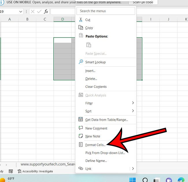
Here you will find a Fill tab at the top of the window that you can use to change the cell background color. You can even click the More Colors button here if you would like to use a color code to modify the color of the cell.
One other option that you can consider to highlight data with cell colors is to apply conditional formatting. This lets you choose a conditional format based on the cell value so that Excel will format only cells that fit those criteria.
For example, you could choose to format cell values over zero with a green color and make a red cell if it contains a value below zero, or you could apply background colors based on the selected cells containing certain words.
You can find the Conditional Formatting option on the Home tab in the Styles section of the ribbon. Simply click the Conditional Formatting button, choose the parameters, and select format options based on how you want excel to color in your cells.
The rules applied during the process of setting up the conditional formatting parameters will apply the cell color based on the options you select.
If none of the color code based options that you see on this dropdown menu offer the solution that you are looking for, then you could click the New rule button and choose your own format.
If you are using Google Sheets and want to be able to color cells, then you are also able to do that. Simply open the spreadsheet in Google Sheets, select the cells that you wish to color, then click the Fill Color button in the toolbar above the spreadsheet. You could also click the Format button at the top of the window and use Conditional formatting or alternating colors there for some more advanced methods of coloring spreadsheet cells.
Additional Sources

Matthew Burleigh has been writing tech tutorials since 2008. His writing has appeared on dozens of different websites and been read over 50 million times.
After receiving his Bachelor’s and Master’s degrees in Computer Science he spent several years working in IT management for small businesses. However, he now works full time writing content online and creating websites.
His main writing topics include iPhones, Microsoft Office, Google Apps, Android, and Photoshop, but he has also written about many other tech topics as well.
Read his full bio here.