
Содержание
- AutoFill and Flash Fill
- Want more?
- Excel Fill
- Filling
- How To Fill
- Fill Copies
- Fill Sequences
- Sequence of Dates
- Combining Words and Letters
- How to Fill Blank Cells with Value above in Excel?
- How to Fill Blank Cells with Value above in Excel
- Fill Cells with Value Above Using ‘Go To Special’ + Formula
- Fill Cells with Value Above Using ‘Find and Replace’ + Formula
- Fill Cells with Value Above Using VBA
AutoFill and Flash Fill

Watch this video for a quick introduction to AutoFill and Flash Fill, two helpful time savers that we’ll cover in more detail in this course.
Want more?
Sometimes you need to enter a lot of repetitive information in Excel, such as dates, and it can be really tedious.
If you think there might be an easier, automated way to do this, you’d be right.
Type the first date in the series.
Put the mouse pointer over the bottom right-hand corner of the cell until it’s a black plus sign.
Click and hold the left mouse button, and drag the plus sign over the cells you want to fill.
And the series is filled in for you automatically using the AutoFill feature.
Or, say you have information in Excel that isn’t formatted the way you need it to be, such as this list of names.
Going through the entire list manually to correct them is daunting.
You’d think there’d be an easier automated way to do this, too, and you’d be right again.
Type the first name the way you want it.
Start to type the next name, and, as if by magic, Excel provides a preview of the names formatted the way you want.
Press Enter, and the names are all filled in for you using the Flash Fill feature, which is new in Excel 2013.
AutoFill and Flash Fill are tremendous time savers, and they can do much more than we have covered in this introduction.
In the next videos, we’ll cover them in more detail.
Источник
Excel Fill
Filling
Filling makes your life easier and is used to fill ranges with values, so that you do not have to type manual entries.
Filling can be used for:
For now, do not think of functions. We will cover that in a later chapter.
How To Fill
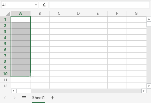
Filling is done by selecting a cell, clicking the fill icon and selecting the range using drag and mark while holding the left mouse button down.
The fill icon is found in the button right corner of the cell and has the icon of a small square. Once you hover over it your mouse pointer will change its icon to a thin cross.
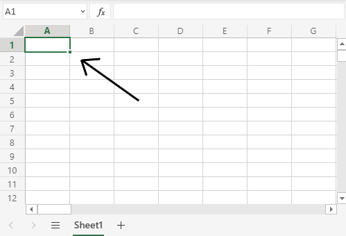
Click the fill icon and hold down the left mouse button, drag and mark the range that you want to cover.
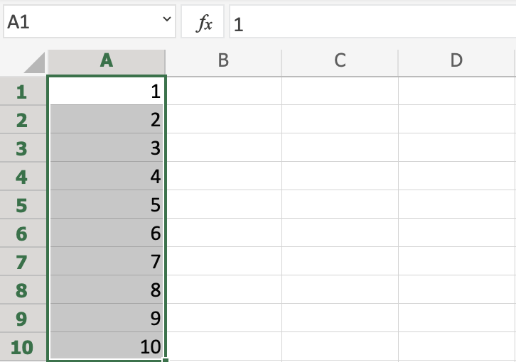
In this example, cell A1 was selected and the range A1:A10 was marked.
Now that we have learned how to fill. Let’s look into how to copy with the fill function.
Fill Copies
Filling can be used for copying. It can be used for both numbers and words.
Let’s have a look at numbers first.
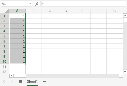
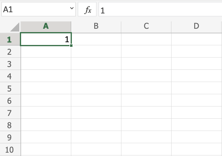
In this example we have typed the value A1(1) :
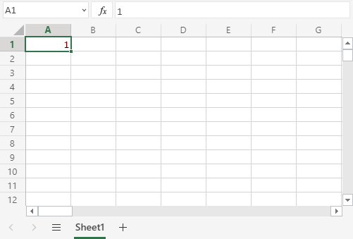
Filling the range A1:A10 creates ten copies of 1:
The same principle goes for text.
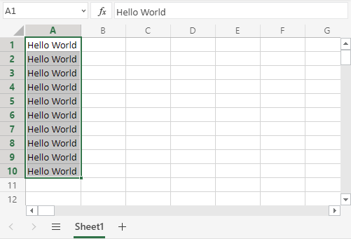
In this example we have typed A1(Hello World) .
Filling the range A1:A10 creates ten copies of «Hello World»:
Now you have learned how to fill and to use it for copying both numbers and words. Let’s have a look at sequences.
Fill Sequences
Filling can be used to create sequences. A sequence is an order or a pattern. We can use the filling function to continue the order that has been set.
Sequences can for example be used on numbers and dates.
Let’s start with learning how to count from 1 to 10.
This is different from the last example because this time we do not want to copy, but to count from 1 to 10.
Start with typing A1(1) :
First we will show an example which does not work, then we will do a working one. Ready?
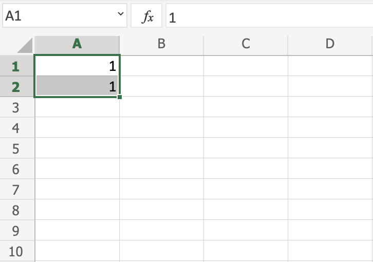
Lets type the value ( 1 ) into the cell A2 , which is what we have in A1 . Now we have the same values in both A1 and A2 .
Let’s use the fill function from A1:A10 to see what happens. Remember to mark both values before you fill the range.
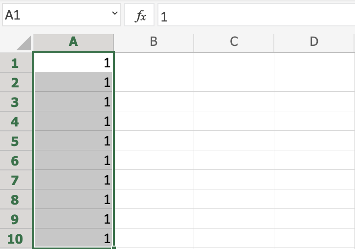
What happened is that we got the same values as we did with copying. This is because the fill function assumes that we want to create copies as we had two of the same values in both the cells A1(1) and A2(1) .
Change the value of A2(1) to A2(2) . We now have two different values in the cells A1(1) and A2(2) . Now, fill A1:A10 again. Remember to mark both the values (holding down shift) before you fill the range:
Congratulations! You have now counted from 1 to 10.
The fill function understands the pattern typed in the cells and continues it for us.
That is why it created copies when we had entered the value ( 1 ) in both cells, as it saw no pattern. When we entered ( 1 ) and ( 2 ) in the cells it was able to understand the pattern and that the next cell A3 should be ( 3 ).
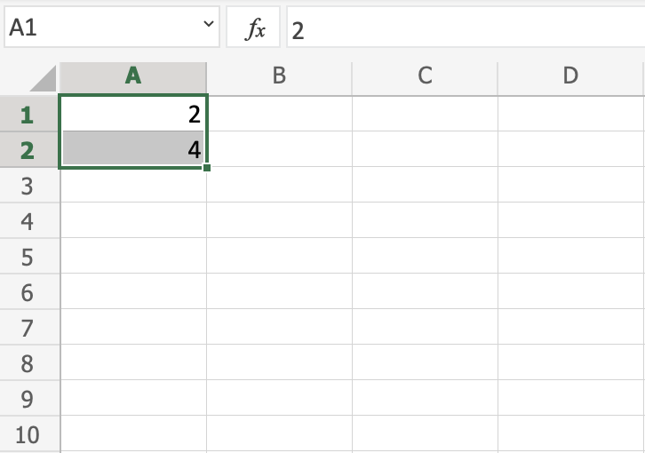
Let’s create another sequence. Type A1(2) and A2(4) :
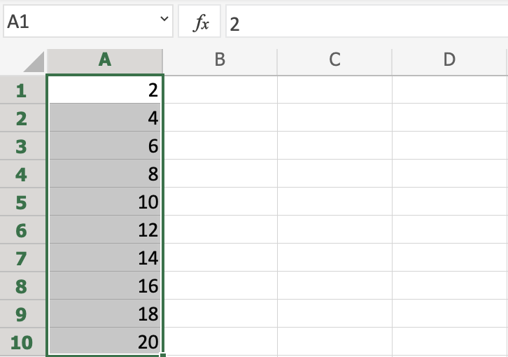
It counts from 2 to 20 in the range A1:A10 .
This is because we created an order with A1(2) and A2(4) .
Then it fills the next cells, A3(6) , A4(8) , A5(10) and so on. The fill function understands the pattern and helps us continue it.
Sequence of Dates
The fill function can also be used to fill dates.
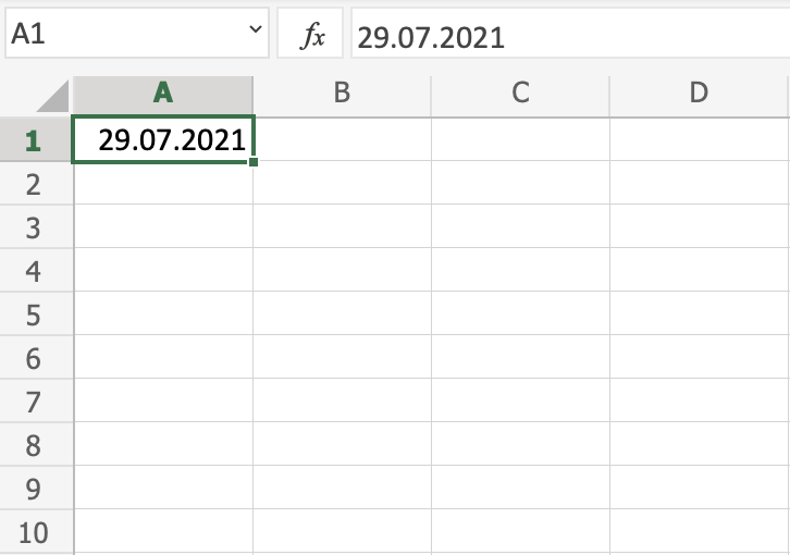
Test it by typing A1(29.07.2021) :
And fill the range A1:A10 :
The fill function has filled 10 days from A1(29.07.2021) to A10(07.08.2021) .
Note that it switched from July to August in cell A4 . It knows the calendar and will count real dates.
Combining Words and Letters
Words and letters can also be combined.
Type A1(Hello 1) and A2(Hello 2) :
Next, fill A1:A10 to see what happens:
The result is that it counts from A1(Hello 1) to A10(Hello 10) . Only the numbers have changed.
It recognised the pattern of the numbers and continued it for us. Words and numbers can be combined, as long as you use a recognizable pattern for the numbers.
Источник
How to Fill Blank Cells with Value above in Excel?
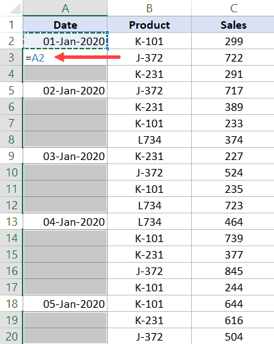
Sometimes, you may have a dataset where there are empty/blank cells in a dataset that should have been filled with the same value.
Below is a common example where the date is only mentioned one time and all the remaining records for that same date have the date cells blank.
While this type of data may look cleaner (especially when printed), it’s not great when you try to use this for calculations or create a Pivot Table using it.
In many cases, you would need to fill these blank cells with the value in the above cell.
Table of Contents
How to Fill Blank Cells with Value above in Excel
In this Excel tutorial, I will show you three really easy ways to fill the blank cells with the value above in Excel.
- Using Go To Special with a formula
- Using Find and Replace with a formula
- Using VBA
The tricky part of this entire process is actually selecting the blank cells. Once you have the blank cells selected, there are multiple ways to copy cell values from above.
So let’s get started!
Fill Cells with Value Above Using ‘Go To Special’ + Formula
The first step in filling blank cells from the value above is to select these blank cells. And this can easily be done using the ‘Go To Special’ option in Excel.
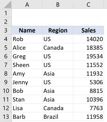
Suppose you have a dataset as shown below and you want to fill all the blank cells in column A with the date from the cell above.
![]()
Below are the steps to select all these blank cells at one go:
- Select the dataset in which you have these blank/empty cells
- Hit the F5 key on your keyboard (use ⌃ + G if you’re using a Mac). This will open the ‘Go To’ dialog box
- Click on the Special button.
- In the ‘Go To Special’ dialog box, select the ‘Blanks’ option

- Click OK.
The above steps would select all the blank cells in this dataset.
![]()
Now that you have all the blank cells selected, the next step is to fill all these blank cells from the value above.
Follow the following steps to use a formula to copy the value from the cell above:
- Enter = (equal to sign). by default, this will enter the equal to sign in the active cell only
- Press the up-arrow key. This will select the cell right above the active cell
- Hold the Control key and press the enter key (Command + Enter if you’re using a Mac)
The above steps would apply the same formula (which is simply to refer to the cell above) to all the selected blank cells.
Once you have all these blank cells filled, remember to convert the formulas to values.
Fill Cells with Value Above Using ‘Find and Replace’ + Formula
The above (Go To Special) method works well when you only have the blank cells that you want to fill-down.
But what if you get a dataset where the cells are not really blank (but may have a dash in it or some text such as NA).
In such a case, you can also use the Find and Replace method.
This method works similar to Go To Special, but with an added advantage of being able to select cells based on the value.
With this method, you can select blank cells or you can select cells that have any specific text/value in it.
Let me show you how this would work taking an example of blank cells only.
Suppose you have a dataset as shown below and you want to fill all the blank cells in column A with the date from the cell above.
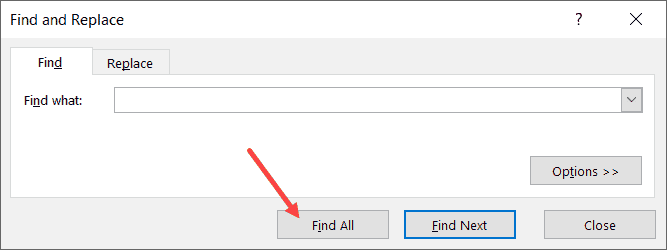
Below are the steps to select all the blank cells using Find and Replace:
- Select the dataset in which you have these blank/empty cells
- Hold the Control key and press the F key (or Command + F if you’re using Mac)
- In the Find and Replace dialog box that opens up, click on the ‘Find All’ button. This will find all the cells that are blank and you will also see a list of these cells addresses.
- Hold the Control key and press the A key (or Command + A if you’re using Mac). This will select all these blank cells
- Close the Find and Replace dialog box.
By the end of these steps, you will have all the empty cells selected.
Now, you can use the formula to get the value from the above cell and fill in the blank cells in Excel.
Follow the following steps to use a formula to copy the value from the cell above:
- Enter = (equal to sign). by default, this will enter the equal to sign in the active cell only
- Press the up-arrow key. This will select the cell right above the active cell
- Hold the Control key and press the enter key (Command + Enter if you’re using a Mac)
One of the benefits of using Find and Replace it works when you have blank cells that you want to fill, and you can also use it to find and select cells that have specific values.
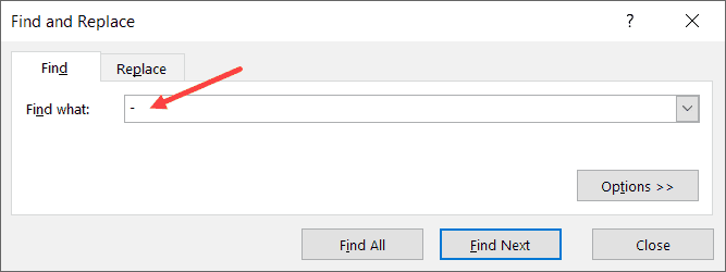
For example, suppose you have a dataset as shown below where instead of the blank cells, we have dashes instead.
![]()
To do this, follow the below steps:
- Select the dataset
- Hold the Control key and press the F key (or Command + F if you’re using Mac)
- In the Find and Replace dialog box that opens up, enter – (dash) in the ‘Find what’ field.
- Click on the Find All button. This will find all the cells that have the dash symbol and you will also see a list of these cells’ addresses.
- Hold the Control key and press the A key (or Command + A if you’re using Mac). This will select all these cells
- Close the Find and Replace dialog box.
Once you have these cells selected, you can use the formula steps shown above to fill values from cells above (or even full cell values from below/right/left).
Fill Cells with Value Above Using VBA
While these two above methods work perfectly fine, in case you have to do this quite often, you can also use a simple VBA code to get this done.
And if you want to be super-efficient and get this done with a single click, you can add the VBA macro to the Quick Access Toolbar (QAT) and simply click on it to fill the blank cells in the selection with the cell value from the above cell.
Below is the VBA code that will get this done:
To use this code, first, select the dataset where you want to copy the value from the above cell, and then run this code.
The above code uses the FOR EACH loop where it goes through each and every cell in the selection. As soon as it finds a cell that’s empty (checked using the IF statement), it copies the value from the cell above (done using OFFSET).
In this specific example, you may notice that
Note: In case you want to save a workbook that has the macro code, you need to save it in the .XLSM (macro enabled) format.
The best thing about using this VBA code is that it doesn’t require you to convert the formulas into values. With this method, you get static values only. This makes it a really efficient method (of all the three covered in this tutorial).
There are however two things you need to know when using VBA to get fill the blank cells with a value from the above cell:
- You can’t undo this once you have run the macro code. So make sure you create a backup copy before you run the VBA code
- If you have a huge dataset (thousands of rows with multiple columns), this is likely to slow down your system. Since the VBA code above goes through and analyzes each cell, it takes more time than the remaining two methods. When using with a few hundred (or even a few thousand data points), you’ll likely not notice any difference in speed.
To use this VBA macro code, you need to put it into a regular module.
So these are three ways you can use to fill the blank cells with data from the cell above it.
Hope you found this tutorial useful!
You may also like the following Excel tutorials:
Источник
-
01-27-2007, 02:39 PM
#1
Registered User
Autofill «fill as you type» Lookups
I have searched previous messages but do not see exactly what I need:
Lets say I have a file named Book1.xls.
Cell A1 is where I will type data which looks up data from a list (A10:A20) described below.
Cells A10:A20 contain a list of values;
Bob
Don
Jack
Jerry
Jill
Ralph
ect…What I would like to happen is:
As soon I start to type letters into Cell A1, (for instance) «J» the cell would automatically fill the cell with the value that most closely matches the item in the list located at A10:A20. In this case «J» would result in «Jack» in cell A1.
Lets then say that if I continue to type «JE», the result in cell A1 would be «Jerry».
I have seen examples on the internet that employ the use of a combo box and VB code. However, those examples require that cell A1 be double clicked on with the mouse in order to display (pop up) the combo box.
Is anyone able to show me an example using my sample data which does not reqiure doing anything but simply typing data into cell A1 to achieve the desired results?
Thanks in advance
Mark
Redding California
-
01-27-2007, 08:00 PM
#2
You might not be able to tell from the first few posts in the thread, but this one has an example that does what you ask for, and several references explaining how it works.
http://www.excelforum.com/showthread.php?t=585952
-
01-27-2007, 08:15 PM
#3
Registered User
Originally Posted by MSP77079Thank you for your reply. However I have seen that example and it requires double clicking on the cell in order for the combo box to appear, which is set up for auto completion.
I was looking for an example that makes this happen without double or single clicking the cell to force the combo box open.
Thank you again
Mark
-
01-28-2007, 12:15 AM
#4
My first thought on reading your second posting is that it is impossible. But, after letting it roll around in my head for a few hours, I realized it is very easy. Sort of. If you can accept a compromise
You have probably noticed before that Excel does this automatically (and somewhat maddeningly) when you have a long list of items in a column. You start typing, and if the item is already in the list, it will autocomplete for you. (You can turn if off; Tools >> Options, see the Edit tab, last selection.)
So, what you need to do is turn your sheet upside down. Instead of putting the list of names in Cells A10:A20 and you start typing in A1 … you put the list of names in A1 to A21; then hide those rows, and you start typing in cell A22.
-
01-28-2007, 04:08 AM
#5
Registered User
Interesting suggestion.
I have downloaded a sample file that requires the doubleclick and am including the VB code for your review. It seems to me the the event;
Private Sub Worksheet_BeforeDoubleClick(ByVal Target As Range, Cancel As Boolean) could be replaced with something like; Worksheet_Cell_OnEnter ??? Of course, that event does not exist in Excel.Below is the code, what do you think?
Option Explicit
Private Sub TempCombo_KeyDown(ByVal _
KeyCode As MSForms.ReturnInteger, _
ByVal Shift As Integer)
‘Hide combo box and move to next cell on Enter and Tab
Select Case KeyCode
Case 9
ActiveCell.Offset(0, 1).Activate
Case 13
ActiveCell.Offset(1, 0).Activate
Case Else
‘do nothing
End SelectEnd Sub
Private Sub Worksheet_BeforeDoubleClick(ByVal Target As Range, Cancel As Boolean)
Dim str As String
Dim cboTemp As OLEObject
Dim ws As Worksheet
Set ws = ActiveSheet
Cancel = True
Set cboTemp = ws.OLEObjects(«TempCombo»)
On Error Resume Next
With cboTemp
.ListFillRange = «»
.LinkedCell = «»
.Visible = False
End With
On Error GoTo errHandler
If Target.Validation.Type = 3 Then
Application.EnableEvents = False
str = Target.Validation.Formula1
str = Right(str, Len(str) — 1)
With cboTemp
.Visible = True
.Left = Target.Left
.Top = Target.Top
.Width = Target.Width + 15
.Height = Target.Height + 5
.ListFillRange = ws.Range(str).Address
.LinkedCell = Target.Address
End With
cboTemp.Activate
End IferrHandler:
Application.EnableEvents = True
Exit SubEnd Sub
Private Sub Worksheet_SelectionChange(ByVal Target As Range)
Dim str As String
Dim cboTemp As OLEObject
Dim ws As Worksheet
Set ws = ActiveSheetSet cboTemp = ws.OLEObjects(«TempCombo»)
On Error Resume Next
If cboTemp.Visible = True Then
With cboTemp
.Top = 10
.Left = 10
.ListFillRange = «»
.LinkedCell = «»
.Visible = False
.Value = «»
End With
End IferrHandler:
Application.EnableEvents = True
Exit SubEnd Sub
-
01-28-2007, 12:44 PM
#6
Not really … what you really want is a «KeyUp» event. In other words, you want to trap each time the user FINISHES a keystroke.
As you point out, there is no such event in Excel. Not in the worksheet events (which are easily coded), not in the workbook events (which are easily coded), not in the application events (which require using a Class Module, therefore are more difficult to code). This event DOES exist for ActiveX objects (such as a TextBox) and for Forms. But, you want to avoid using an ActiveX object because it is not quite as seamless as entering directly into text.
This event also exists, of course for the Windows operating system. So, one could trap this event at the operating system level. This is called Subclassing or Hooking (depending on where in the Windows operating system you choose to insert your code).
I have subclassed Excel before. But, there is a problem doing this with Excel. There are SO MANY events that Excel already traps and responds to that if you subclass a visible window in Excel, you will end up freezing the application. At least if you use VBA for doing the subclassing. (I have sucessfully subclassed a minimized Excel window to trap and discard any messages that would make the window visible or give it focus.)
If your intent is to fill a column with validated data, in a way that allows auto-complete, and avoids the need to continually double click to display the combo-box … might I suggest that you use instead a non-modal form. You open the form with the double-click (or some other way, such as a hot-key like Ctrl+some key, or a button, or a right-click); but, the form stays open until you dismiss it.


How to control AutoComplete in Excel
Updated on December 12, 2020
What to Know
- Excel 2019 to 2010: Go to File > Options > Advanced. Under Editing Options, toggle Enable AutoComplete for cell values on or off.
- Excel 2007: Click the Office Button > Excel Options > Advanced. Select or unselect Enable AutoComplete for cell values.
- Excel 2003: Go to Tools > Options > Edit. Select or unselect Enable AutoComplete for cell values.
This article explains how to enable or disable the AutoComplete option in Microsoft Excel, which will automatically fill in data as you type. Instructions cover Excel 2019, 2016, 2013, 2010, 2007, and 2003.
Enable/Disable AutoComplete in Excel
The steps for enabling or disabling AutoComplete in Microsoft Excel are different depending on the version you’re using:
In Excel 2019, 2016, 2013, and 2010
-
Navigate to the File > Options menu.
-
In the Excel Options window, open Advanced on the left.
-
Under the Editing Options section, toggle Enable AutoComplete for cell values on or off depending on whether you want to turn this feature on or disable it.
Lifewire
-
Click or tap OK to save the changes and continue using Excel.
In Excel 2007
-
Click the Office Button.
-
Choose Excel Options to bring up the Excel Options dialog box.
-
Choose Advanced in the pane to the left.
-
Click the box next to the Enable AutoComplete for cell values option box to turn this feature on or off.
-
Choose OK to close the dialog box and return to the worksheet.
In Excel 2003
-
Navigate to Tools > Options from the menu bar to open the Options dialog box.
-
Choose the Edit tab.
-
Toggle AutoComplete on/off with the checkmark box next to the Enable AutoComplete for cell values option.
-
Click OK to save the changes and return to the worksheet.
When You Should and Shouldn’t Use AutoComplete
AutoComplete is helpful when entering data into a worksheet that contains lots of duplicates. With AutoComplete on, when you start typing, it will auto-fill the rest of the information from the context around it, to speed up data entry.
Say you’re entering the same name, address, or other information into multiple cells. Without AutoComplete, you’d have to retype the data or copy and paste it over and over, which wastes time.
For example, if you typed «Mary Washington» in the first cell and then many other things in the following ones, like «George» and «Harry,» you can type «Mary Washington» again a lot faster by just typing «M» and then pressing Enter so that Excel will auto-type the full name.
You can do this with any number of text entries in any cell in any series, meaning that you could then type «H» at the bottom to have Excel suggest «Harry,» and then type «M» again if you need to have that name auto-completed. There’s no need to copy or paste any data.
However, AutoComplete isn’t always your friend. If you don’t need to duplicate anything, it will still auto-suggest it each time you start typing something that shares the same first letter as the previous data, which can often be more of a bother than a help.
Thanks for letting us know!
Get the Latest Tech News Delivered Every Day
Subscribe
Excel has some powerful Filter options (with inbuilt filter, advanced filter, and now the FILTER function in Office 365).
But none of these options actually filter as you type (i.e., show you the filtered data dynamically while you’re typing).
Something as shown below:
Although there is no inbuilt filter feature to do this, you can easily create something like this in Excel.
In this Excel tutorial, I will show you two simple ways to filter as you type in Excel.
The first method will be using the FILTER function (which you can access only in Office 365, now called Microsoft 365) and the other method would be by using a simple VBA code.
So let’s get started!
Filter as You Type (Using FILTER Function, No VBA Needed)
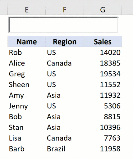
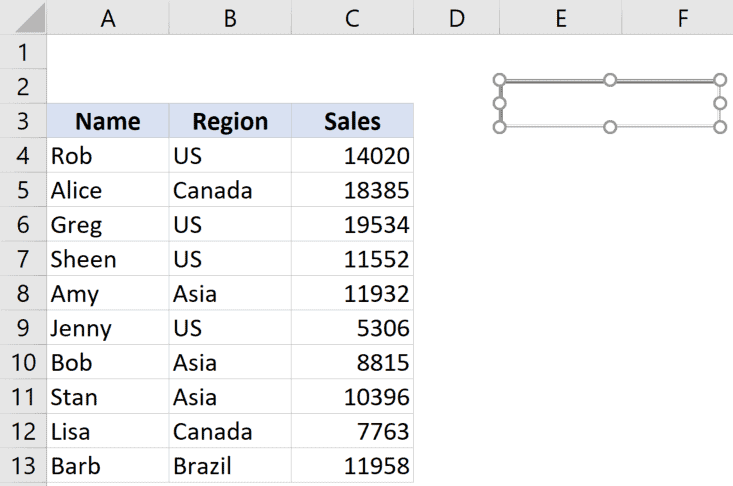
Suppose you have a dataset as shown below and you want to quickly filter data based on the region as you’re typing in a search box (which we will insert in the worksheet).
The first step is to insert a text box where you can type a text string and it will use it to filter the data (while you’re typing).
Below are the steps to insert the text box:
- Click the Developer tab.

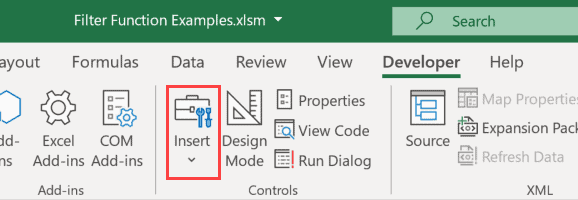
- In the Control group, click on Insert.
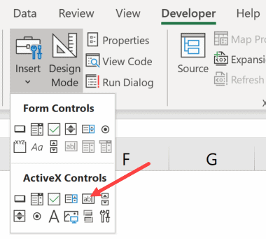
- Click on the Text Box icon in the ActiveX Controls

- Place the cursor anywhere in the worksheet, click and drag. This will insert a text box in the worksheet. You can place this text box wherever you want and can also resize it.

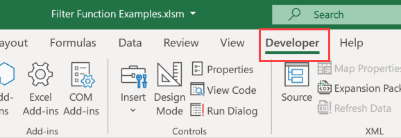
In case you don’t see the Developer tab in the ribbon (in Step 1), right-click on any of the tabs and click on ‘Customize the Ribbon’. In the Excel Options dialog box that opens, check the Developer option in the right pane and click OK. This will make the Developer tab visible in the ribbon.
Now that we have the text box in the worksheet, the next step is to connect it to a cell in the worksheet so that when you type anything in the worksheet, it will also automatically be entered in a cell.
This will allow us to use the value in the cell to filter the data.
Below are the steps to link the text box to a cell:
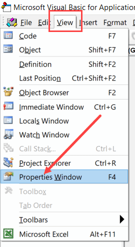
- Double-click on the text box. This will open the VB Editor.
- Click the View option in the menu and then click on Properties Window. This will show the Properties Window Pane for the text box.

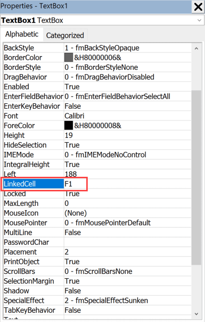
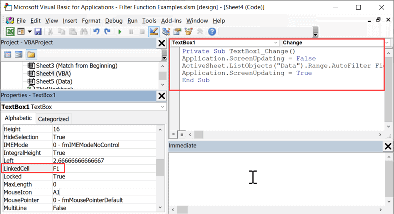
- In the properties window, come to the Linked Cell option and enter F1. This is the cell that we are connecting to the text box

- Close the VB Editor
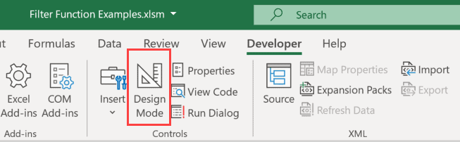
- Go to the Developer tab, and click on the Design mode. You will notice that it turns from dark gray to light gray (indicating that it’s not enabled now).

Now, when you enter any text in the text box, you will notice that it appears in cell E1 in real-time (as you’re typing)
Now that we have linked the text box to a cell, the last step is to filter the data based on the value in the text box (which in turn would be the value in cell E1)
For this, we need to enter the FILTER formula in cell E4, so that results are filtered and shown there.
Below is the formula that will now filter the results as soon you can enter anything in the text box:
=FILTER(A4:C13,ISNUMBER(SEARCH(E1,B4:B13)))
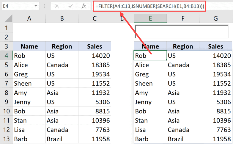
The above formula uses the FILTER function with the array as the original dataset and the condition uses the SEARCH formula.
The SEARCH formula checks whether the value entered in the text box (which also automatically gets entered in cell E1) is there in the cells in column B or not. All the cells that have the text will return a number and those that don’t will return the #VALUE! error.
The ISNUMBER function is used to get TRUE if there is a match and the cell returns a number, and FALSE is it returns the error.
Based on this condition, the data is filtered as you type.
Note that this formula checks whether the text string entered in the text box appears in the cells in column B or not. For example, if you enter ‘a’ in the text box, it would return all the records for Canada, Asia, and Brazil.
The position of the text string in the cells in column B is not checked.
In case you want to have the text string (that you enter in the search box) at the beginning only, you can use the below formula instead:
=FILTER(A4:C13,LEFT(B4:B13,LEN(E1))=E1)
Now when you enter A in the search box, it will only give you records for Asia.
If you’re not using Office 365 and don’t have access to the FILTER function, you can still create the ‘filter as you type’ search box in Excel.
This can be done by using a really simple VBA code mentioned below:
Private Sub TextBox1_Change()
Application.ScreenUpdating = False
ActiveSheet.ListObjects("Data").Range.AutoFilter Field:=2, Criteria1:= "*" & [A1] & "*", Operator:=xlFilterValues
Application.ScreenUpdating = True
End Sub
To use this code, you will have to first insert the text box in the worksheet and then add this code for the text box.
But the first step is to convert the data into an Excel table. While you can use this code without converting the data into an Excel table, it will be easier when the data is in Table as it becomes easier to refer to in the VBA code.
Below are the steps to convert the data into an Excel table:
- Select any cell in the dataset
- Hold the Control key and press the T key (or Command + T if you’re using a Mac).
- In the Create Table dialog box that opens, check whether the range is correct or not.
- Click Ok
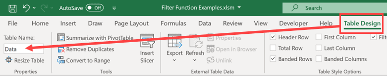
- Select any cell in the Excel Table
- Click on the ‘Table Design’ tab
- Change the name of the table to Data. You can use any name you want, but make sure to use the same one in the VBA code as well.

Below are the steps to insert the text box in the worksheet:
- Click the Developer tab.
- In the Control group, click on Insert.
- Click on the Text Box icon in the ActiveX Controls
- Place the cursor anywhere in the worksheet, click and drag. This will insert a text box in the worksheet. You can place this text box wherever you want and can also resize it.
Now that you have the text box in the sheet, you need to connect to a cell and then add the VBA code to the text box code window.
Below are the steps to do this:
- Double-click on the text box. This will open the VB Editor.
- Click the View option in the menu and then click on Properties Window. This will show the Properties Window Pane for the text box.
- In the properties window, come to the Linked Cell option and enter F1. This is the cell that we are connecting to the text box
- In the code window of the Text Box, copy and paste the above VBA code

- Close the VB Editor
- Go to the Developer tab, and click on the Design mode. You will notice that it turns from dark gray to light gray (indicating that it’s not enabled now).
Now you have a text box that is linked to a cell and this cell is used in the VBA code to filter the data.
When you enter any text in the text box, you will see that it filters the table in real tile (filter the data as you type in the text box).
Note: Since the VBA code is executed every time you enter a character in the text box, this method could make your workbook slightly slow in case you have a large data set. In such a case, instead of using the code in the text box code window, you can use it in a regular module and then assign it to a button. That way, you can first type the text in the text box and then click on the button to filter the data.
So these are two methods you can use to create a dynamic filter in Excel (filter data as you type).
Hope you found this tutorial useful!
You may also like the following Excel tutorials:
- How to Clear Contents in Excel without Deleting Formulas
- How to Clear Filter in Excel? Shortcut!
- How to Hide Rows based on Cell Value in Excel
- How to Unhide All Rows in Excel with VBA
- How to Delete a Sheet in Excel Using VBA
- How to Select Alternate Columns in Excel (or every Nth Column)
- How to Select Every Other Cell in Excel (Or Every Nth Cell)
- How to Paste in a Filtered Column Skipping the Hidden Cells
Filling
Filling makes your life easier and is used to fill ranges with values, so that you do not have to type manual entries.
Filling can be used for:
- Copying
- Sequences
- Dates
- Functions (*)
For now, do not think of functions. We will cover that in a later chapter.
How To Fill
Filling is done by selecting a cell, clicking the fill icon and selecting the range using drag and mark while holding the left mouse button down.
The fill icon is found in the button right corner of the cell and has the icon of a small square. Once you hover over it your mouse pointer will change its icon to a thin cross.
Click the fill icon and hold down the left mouse button, drag and mark the range that you want to cover.
In this example, cell A1 was selected and the range A1:A10 was marked.
Now that we have learned how to fill. Let’s look into how to copy with the fill function.
Fill Copies
Filling can be used for copying. It can be used for both numbers and words.
Let’s have a look at numbers first.
In this example we have typed the value A1(1):
Filling the range A1:A10 creates ten copies of
1:
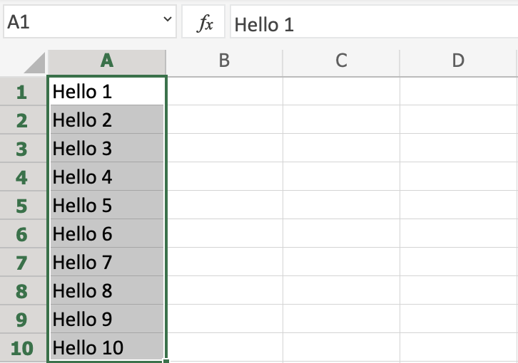
The same principle goes for text.
In this example we have typed A1(Hello World).
Filling the range A1:A10 creates ten copies of «Hello World»:
Now you have learned how to fill and to use it for copying both numbers and words. Let’s have a look at sequences.
Fill Sequences
Filling can be used to create sequences. A sequence is an order or a pattern. We can use the filling function to continue the order that has been set.
Sequences can for example be used on numbers and dates.
Let’s start with learning how to count from 1 to 10.
This is different from the last example because this time we do not want to copy, but to count from 1 to 10.
Start with typing A1(1):
First we will show an example which does not work, then we will do a working one. Ready?
Lets type the value (1) into the cell A2, which is what we have in A1. Now we have the same values in both A1 and A2.
Let’s use the fill function from A1:A10 to see what happens. Remember to mark both values before you fill the range.
What happened is that we got the same values as we did with copying. This is because the fill function assumes that we want to create copies as we had two of the same values in both the cells A1(1) and A2(1).
Change the value of A2(1) to A2(2). We now have two different values in the cells A1(1) and A2(2). Now, fill A1:A10
again. Remember to mark both the values (holding down shift) before you fill the
range:
Congratulations! You have now counted from 1 to 10.
The fill function understands the pattern typed in the cells and continues it for us.
That is why it created copies when we had entered the value (1) in both cells,
as it saw no pattern. When we entered (1) and (2) in the cells it was able to understand the pattern and that the next cell A3 should be (3).
Let’s create another sequence. Type A1(2) and A2(4):
Now, fill A1:A10:
It counts from 2 to 20 in the range A1:A10.
This is because we created an order with A1(2) and A2(4).
Then it fills the next cells, A3(6), A4(8), A5(10) and so on. The fill function understands the pattern and helps us continue it.
Sequence of Dates
The fill function can also be used to fill dates.
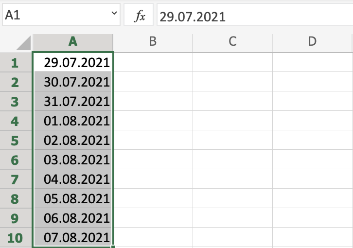
Test it by typing A1(29.07.2021):
And fill the range A1:A10:
The fill function has filled 10 days from A1(29.07.2021) to A10(07.08.2021).
Note that it switched from July to August in cell A4. It knows the calendar and will count real dates.
Combining Words and Letters
Words and letters can also be combined.
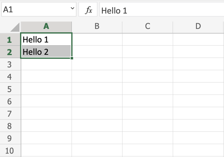
Type A1(Hello 1) and A2(Hello 2):
Next, fill A1:A10 to see what happens:
The result is that it counts from A1(Hello 1) to A10(Hello 10). Only the numbers have changed.
It recognised the pattern of the numbers and continued it for us. Words and numbers can be combined, as long as you use a recognizable pattern for the numbers.