

Sorting data is an integral part of data analysis. You might want to arrange a list of names in alphabetical order, compile a list of product inventory levels from highest to lowest, or order rows by colors or icons. Sorting data helps you quickly visualize and understand your data better, organize and find the data that you want, and ultimately make more effective decisions.
You can sort data by text (A to Z or Z to A), numbers (smallest to largest or largest to smallest), and dates and times (oldest to newest and newest to oldest) in one or more columns. You can also sort by a custom list you create (such as Large, Medium, and Small) or by format, including cell color, font color, or icon set.
Notes:
-
To find the top or bottom values in a range of cells or table, such as the top 10 grades or the bottom 5 sales amounts, use AutoFilter or conditional formatting.
-
For more information, see Filter data in an Excel table or range, and Apply conditional formatting in Excel .

Sort text
-
Select a cell in the column you want to sort.
-
On the Data tab, in the Sort & Filter group, do one of the following:
-
To quick sort in ascending order, click
 (Sort A to Z).
 -
To quick sort in descending order, click
(Sort Z to A).
-
 (Sort A to Z).
 (Sort Z to A).
Notes:
Potential Issues
-
Check that all data is stored as text If the column that you want to sort contains numbers stored as numbers and numbers stored as text, you need to format them all as either numbers or text. If you do not apply this format, the numbers stored as numbers are sorted before the numbers stored as text. To format all the selected data as text, Press Ctrl+1 to launch the Format Cells dialog, click the Number tab and then, under Category, click General, Number, or Text.
-
Remove any leading spaces In some cases, data imported from another application might have leading spaces inserted before data. Remove the leading spaces before you sort the data. You can do this manually, or you can use the TRIM function.
-
Select a cell in the column you want to sort.
-
On the Data tab, in the Sort & Filter group, do one of the following:
-
To sort from low to high, click
(Sort Smallest to Largest). -
To sort from high to low, click
(Sort Largest to Smallest).
-
Notes:
-
Potential Issue
-
Check that all numbers are stored as numbers If the results are not what you expected, the column might contain numbers stored as text instead of as numbers. For example, negative numbers imported from some accounting systems, or a number entered with a leading apostrophe (‘) are stored as text. For more information, see Fix text-formatted numbers by applying a number format.
-
Select a cell in the column you want to sort.
-
On the Data tab, in the Sort & Filter group, do one of the following:
-
To sort from an earlier to a later date or time, click
(Sort Oldest to Newest). -
To sort from a later to an earlier date or time, click
(Sort Newest to Oldest).
-
Notes:
Potential Issue
-
Check that dates and times are stored as dates or times If the results are not what you expected, the column might contain dates or times stored as text instead of as dates or times. For Excel to sort dates and times correctly, all dates and times in a column must be stored as a date or time serial number. If Excel cannot recognize a value as a date or time, the date or time is stored as text. For more information, see Convert dates stored as text to dates.
-
If you want to sort by days of the week, format the cells to show the day of the week. If you want to sort by the day of the week regardless of the date, convert them to text by using the TEXT function. However, the TEXT function returns a text value, so the sort operation would be based on alphanumeric data. For more information, see Show dates as days of the week.
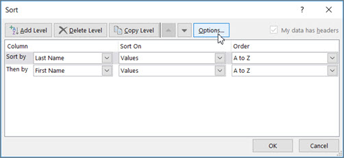
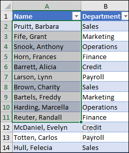
You may want to sort by more than one column or row when you have data that you want to group by the same value in one column or row, and then sort another column or row within that group of equal values. For example, if you have a Department column and an Employee column, you can first sort by Department (to group all the employees in the same department together), and then sort by name (to put the names in alphabetical order within each department). You can sort by up to 64 columns.
Note: For best results, the range of cells that you sort should have column headings.
-
Select any cell in the data range.
-
On the Data tab, in the Sort & Filter group, click Sort.
-
In the Sort dialog box, under Column, in the Sort by box, select the first column that you want to sort.
-
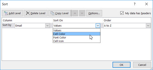
Under Sort On, select the type of sort. Do one of the following:
-
To sort by text, number, or date and time, select Values.
-
To sort by format, select Cell Color, Font Color, or Cell Icon.
-
-
Under Order, select how you want to sort. Do one of the following:
-
For text values, select A to Z or Z to A.
-
For number values, select Smallest to Largest or Largest to Smallest.
-
For date or time values, select Oldest to Newest or Newest to Oldest.
-
To sort based on a custom list, select Custom List.
-
-
To add another column to sort by, click Add Level, and then repeat steps three through five.
-
To copy a column to sort by, select the entry and then click Copy Level.
-
To delete a column to sort by, select the entry and then click Delete Level.
Note: You must keep at least one entry in the list.
-
To change the order in which the columns are sorted, select an entry and then click the Up or Down arrow next to the Options button to change the order.
Entries higher in the list are sorted before entries lower in the list.

If you have manually or conditionally formatted a range of cells or a table column by cell color or font color, you can also sort by these colors. You can also sort by an icon set that you created with conditional formatting.
-
Select a cell in the column you want to sort.
-
On the Data tab, in the Sort & Filter group, click Sort.
-
In the Sort dialog box, under Column, in the Sort by box, select the column that you want to sort.
-
Under Sort On, select Cell Color, Font Color, or Cell Icon.
-
Under Order, click the arrow next to the button and then, depending on the type of format, select a cell color, font color, or cell icon.
-
Next, select how you want to sort. Do one of the following:
-
To move the cell color, font color, or icon to the top or to the left, select On Top for a column sort, and On Left for a row sort.
-
To move the cell color, font color, or icon to the bottom or to the right, select On Bottom for a column sort, and On Right for a row sort.
Note: There is no default cell color, font color, or icon sort order. You must define the order that you want for each sort operation.
-
-
To specify the next cell color, font color, or icon to sort by, click Add Level, and then repeat steps three through five.
Make sure that you select the same column in the Then by box and that you make the same selection under Order.
Keep repeating for each additional cell color, font color, or icon that you want included in the sort.
You can use a custom list to sort in a user-defined order. For example, a column might contain values that you want to sort by, such as High, Medium, and Low. How can you sort so that rows containing High appear first, followed by Medium, and then Low? If you were to sort alphabetically, an “A to Z” sort would put High at the top, but Low would come before Medium. And if you sorted “Z to A,” Medium would appear first, with Low in the middle. Regardless of the order, you always want “Medium” in the middle. By creating your own custom list, you can get around this problem.
-
Optionally, create a custom list:
-
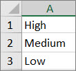
In a range of cells, enter the values that you want to sort by, in the order that you want them, from top to bottom as in this example.
-
Select the range that you just entered. Using the preceding example, select cells A1:A3.
-
Go to File > Options > Advanced > General > Edit Custom Lists, then in the Custom Lists dialog box, click Import, and then click OK twice.
Notes:
-
You can create a custom list based only on a value (text, number, and date or time). You cannot create a custom list based on a format (cell color, font color, or icon).
-
The maximum length for a custom list is 255 characters, and the first character must not begin with a number.
-
-
-
Select a cell in the column you want to sort.
-
On the Data tab, in the Sort & Filter group, click Sort.
-
In the Sort dialog box, under Column, in the Sort by or Then by box, select the column that you want to sort by a custom list.
-
Under Order, select Custom List.
-
In the Custom Lists dialog box, select the list that you want. Using the custom list that you created in the preceding example, click High, Medium, Low.
-
Click OK.
-
On the Data tab, in the Sort & Filter group, click Sort.
-
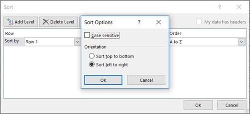
In the Sort dialog box, click Options.
-
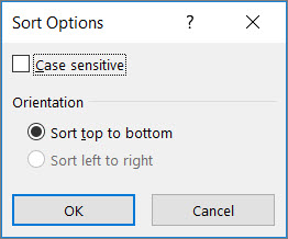
In the Sort Options dialog box, select Case sensitive.
-
Click OK twice.
It’s most common to sort from top to bottom, but you can also sort from left to right.
Note: Tables don’t support left to right sorting. To do so, first convert the table to a range by selecting any cell in the table, and then clicking Table Tools > Convert to range.
-
Select any cell within the range you want to sort.
-
On the Data tab, in the Sort & Filter group, click Sort.
-
In the Sort dialog box, click Options.
-
In the Sort Options dialog box, under Orientation, click Sort left to right, and then click OK.
-
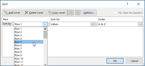
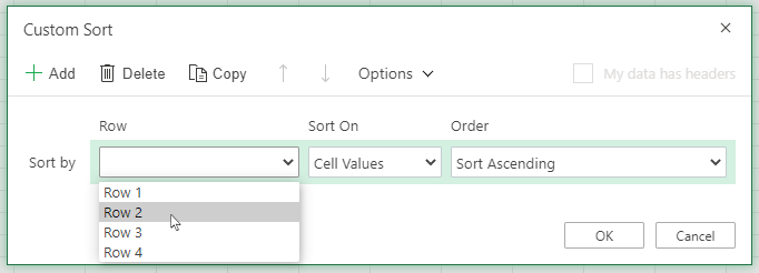
Under Row, in the Sort by box, select the row that you want to sort. This will generally be row 1 if you want to sort by your header row.
Tip: If your header row is text, but you want to order columns by numbers, you can add a new row above your data range and add numbers according to the order you want them.
-
To sort by value, select one of the options from the Order drop-down:
-
For text values, select A to Z or Z to A.
-
For number values, select Smallest to Largest or Largest to Smallest.
-
For date or time values, select Oldest to Newest or Newest to Oldest.
-
-
To sort by cell color, font color, or cell icon, do this:
-
Under Sort On, select Cell Color, Font Color, or Cell Icon.
-
Under Order select a cell color, font color, or cell icon, then select On Left or On Right.
-
Note: When you sort rows that are part of a worksheet outline, Excel sorts the highest-level groups (level 1) so that the detail rows or columns stay together, even if the detail rows or columns are hidden.
To sort by a part of a value in a column, such as a part number code (789-WDG-34), last name (Carol Philips), or first name (Philips, Carol), you first need to split the column into two or more columns so that the value you want to sort by is in its own column. To do this, you can use text functions to separate the parts of the cells or you can use the Convert Text to Columns Wizard. For examples and more information, see Split text into different cells and Split text among columns by using functions.
Warning: It is possible to sort a range within a range, but it is not recommended, because the result disassociates the sorted range from its original data. If you were to sort the following data as shown, the selected employees would be associated with different departments than they were before.
Fortunately, Excel will warn you if it senses you are about to attempt this:

If you did not intend to sort like this, then press the Expand the selection option, otherwise select Continue with the current selection.
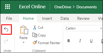
If the results are not what you want, click Undo  .
.
Note: You cannot sort this way in a table.
If you get unexpected results when sorting your data, do the following:
Check to see if the values returned by a formula have changed If the data that you have sorted contains one or more formulas, the return values of those formulas might change when the worksheet is recalculated. In this case, make sure that you reapply the sort to get up-to-date results.
Unhide rows and columns before you sort Hidden columns are not moved when you sort columns, and hidden rows are not moved when you sort rows. Before you sort data, it’s a good idea to unhide the hidden columns and rows.
Check the locale setting Sort orders vary by locale setting. Make sure that you have the proper locale setting in Regional Settings or Regional and Language Options in Control Panel on your computer. For information about changing the locale setting, see the Windows help system.
Enter column headings in only one row If you need multiple line labels, wrap the text within the cell.
Turn on or off the heading row It’s usually best to have a heading row when you sort a column to make it easier to understand the meaning of the data. By default, the value in the heading is not included in the sort operation. Occasionally, you may need to turn the heading on or off so that the value in the heading is or is not included in the sort operation. Do one of the following:
-
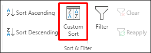
To exclude the first row of data from the sort because it is a column heading, on the Home tab, in the Editing group, click Sort & Filter, click Custom Sort and then select My data has headers.
-
To include the first row of data in the sort because it is not a column heading, on the Home tab, in the Editing group, click Sort & Filter, click Custom Sort, and then clear My data has headers.
If your data is formatted as an Excel table, then you can quickly sort and filter it with the filter buttons in the header row.
-
If your data isn’t already in a table, then format it as a table. This will automatically add a filter button at the top of each table column.
-
Click the filter button at the top of the column you want to sort on, and pick the sort order you want.
-
To undo a sort, use the Undo button on the Home tab.
-
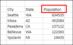
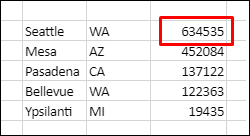
Pick a cell to sort on:
-
If your data has a header row, pick the one you want to sort on, such as Population.
-
If your data doesn’t have a header row, pick the topmost value you want to sort on, such as 634535.
-
-
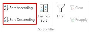
On the Data tab, pick one of the sort methods:
-
Sort Ascending to sort A to Z, smallest to largest, or earliest to latest date.
-
Sort Descending to sort Z to A, largest to smallest, or latest to earliest date.
-
Let’s say you have a table with a Department column and an Employee column. You can first sort by Department to group all the employees in the same department together, and then sort by name to put the names in alphabetical order within each department.
Select any cell within your data range.
-
On the Data tab, in the Sort & Filter group, click Custom Sort.
-
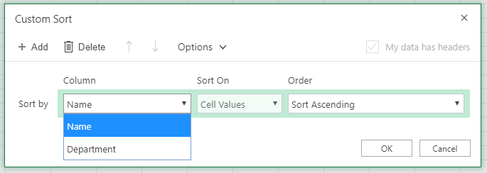
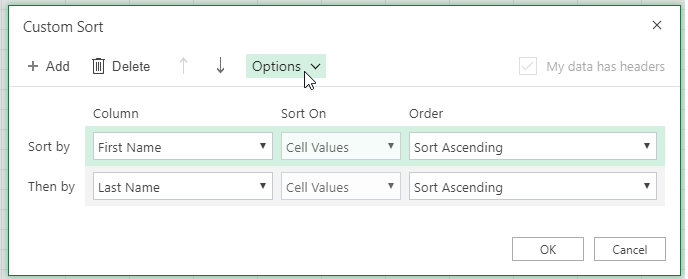
In the Custom Sort dialog box, under Column, in the Sort by box, select the first column that you want to sort.
Note: The Sort On menu is disabled because it’s not yet supported. For now, you can change it in the Excel desktop app.
-
Under Order, select how you want to sort:
-
Sort Ascending to sort A to Z, smallest to largest, or earliest to latest date.
-
Sort Descending to sort Z to A, largest to smallest, or latest to earliest date.
-
-
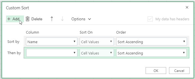
To add another column to sort by, click Add and then repeat steps five and six.
-
To change the order in which the columns are sorted, select an entry and then click the Up or Down arrow next to the Options button.
If you have manually or conditionally formatted a range of cells or a table column by cell color or font color, you can also sort by these colors. You can also sort by an icon set that you created with conditional formatting.
-
Select a cell in the column you want to sort
-
On the Data tab, in the Sort & Filter group, select Custom Sort.
-
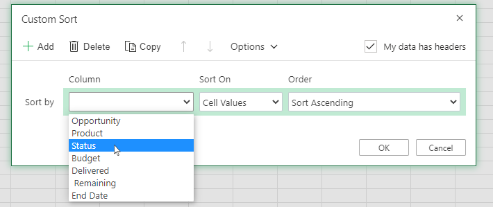
In the Custom Sort dialog box under Columns, select the column that you want to sort.
-
Under Sort On, select Cell Color, Font Color or Conditional Formatting Icon.
-
Under Order, select the order you want (what you see depends on the type of format you have). Then select a cell color, font color, or cell icon.
-
Next, you’ll choose how you want to sort by moving the cell color, font color, or icon:
Note: There is no default cell color, font color, or icon sort order. You must define the order that you want for each sort operation.
-
To move to the top or to the left: Select On Top for a column sort, and On Left for a row sort.
-
To move to the bottom or to the right: Select On Bottom for a column sort, and On Right for a row sort.
-
-
To specify the next cell color, font color, or icon to sort by, select Add Level, and then repeat steps 1- 5.
-
Make sure that you the column in the Then by box and the selection under Order are the same.
-
Repeat for each additional cell color, font color, or icon that you want included in the sort.
-
On the Data tab, in the Sort & Filter group, click Custom Sort.
-
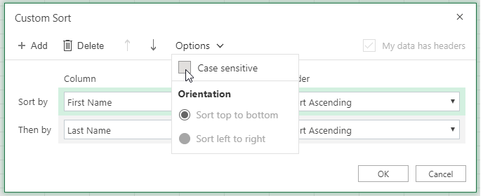
In the Custom Sort dialog box, click Options.
-
In the Options menu, select Case sensitive.
-
Click OK.
It’s most common to sort from top to bottom, but you can also sort from left to right.
Note: Tables don’t support left to right sorting. To do so, first convert the table to a range by selecting any cell in the table, and then clicking Table Tools > Convert to range.
-
Select any cell within the range you want to sort.
-
On the Data tab, in the Sort & Filter group, select Custom Sort.
-
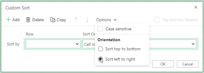
In the Custom Sort dialog box, click Options.
-
Under Orientation, click Sort left to right
-
Under Row, in the ‘Sort by’ drop down, select the row that you want to sort. This will generally be row 1 if you want to sort by your header row.
-
To sort by value, select one of the options from the Order drop-down:
-
Sort Ascending to sort A to Z, smallest to largest, or earliest to latest date.
-
Sort Descending to sort Z to A, largest to smallest, or latest to earliest date
-
Need more help?
You can always ask an expert in the Excel Tech Community or get support in the Answers community.
See also
Use the SORT and SORTBY functions to automatically sort your data.
Listing the files in a folder is one of the activities which cannot be achieved using normal Excel formulas. I could tell you to turn to VBA macros or PowerQuery, but then any non-VBA and non-PowerQuery users would close this post instantly. But wait! Back away from the close button, there is another option.
For listing files in a folder we can also use a little-known feature from Excel version 4, which still works today, the FILES function.
If you search through the list of Excel functions, FILES is not listed. The FILES function is based on an old Excel feature, which has to be applied in a special way. The instructions below will show you step-by-step how to use it.
Create a named range for the FILES function
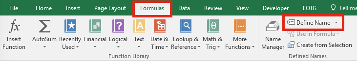
The first step is to create a named range, which contains the FILES function. Within the Excel Ribbon click Formulas -> Define Name
Within the New Name window set the following criteria:
- Name: listFiles
Can be any name you wish, but for our example we will be using listFiles. - Refers to: =FILES(Sheet1!$A$1)
Sheet1!$A$1 is the sheet and cell reference containing the name of the folder from which the files are to be listed.
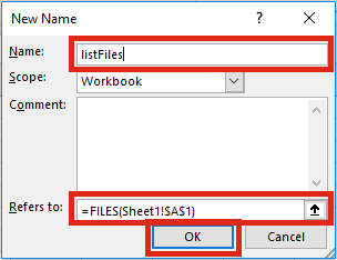
Click OK to close the New Name window.
Apply the function to list files
The second step is to set-up the worksheet to use the named range.
In Cell A1 (or whichever cell reference used in the Refers to box) enter the folder path from which to list the files, followed by an Asterisk ( * ). The Asterisk is the wildcard character to find any text, so it will list all the files in the folder.
Select the cell in which to start the list of files (Cell A3 in the screenshot below), enter the following formula.
=INDEX(listFiles,1)
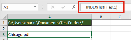
The result of the function will be the name of the first file in the folder.
To retrieve the second file from the folder enter the following formula
=INDEX(listFiles,2)
It would be painful to change the file reference number within each formula individually, especially if there are hundreds of files. The good news is, we can use another formula to calculate the reference number automatically.
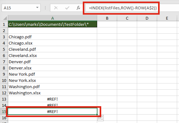
=INDEX(listFiles,ROW()-ROW(A$2))
The ROW() function is used to retrieve the row number of a cell reference. When used without a cell reference, it returns the row number of the cell in which the function is used. When used with a cell reference it returns the row number of that cell. Using the ROWS function, it is possible to create a sequential list of numbers starting at 1, and increasing by 1 for each cell the formula is copied into.
If the formula is copied down further than the number of files in the folder, it will return a #REF! error.
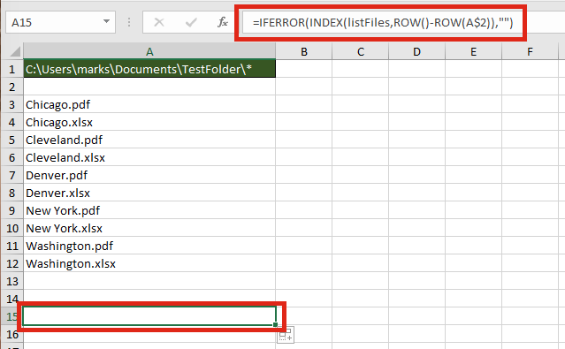
Finally, wrap the formula within an IFERROR function to return a blank cell, rather than an error.
=IFERROR(INDEX(listFiles,ROW()-ROW(A$2)),"")
Listing specific types of files
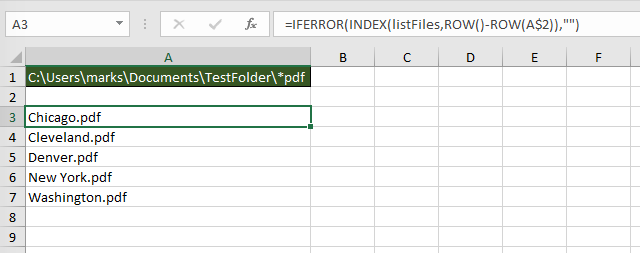
The FILES function does not just list Excel files; it lists all file types; pdf, csv, mp3, zip, any file type you can think of. By extending the use of wildcards within the file path it is possible to restrict the list to specific file types, or to specific file names.
The screenshot below shows how to return only files with “pdf” as the last three characters of the file name.
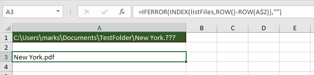
The wildcards which can be applied are:
- Question mark ( ? ) – Can take the place of any single character.
- Asterisk ( * ) – Represents any number of characters
- Tilde ( ~ ) – Used as an escape character to search for an asterisk or question mark within the file name, rather than as a wildcard.
The screenshot below shows how to return only files with the name of “New York.“, followed by exactly three characters.
Advanced uses for the FILES named range
Below are some ideas of how else you could use the FILES function.
Count the number of files
The named range created works like any other named range. However, rather than containing cells, it contains values. Therefore, if you want to calculate the number of files within the folder, or which meet the wildcard pattern use the following formula:
=COUNTA(listFiles)
Create hyperlinks to the files
Wouldn’t it be great to click on the file name to open it automatically? Well . . . just add in the HYPERLINK function and you can.
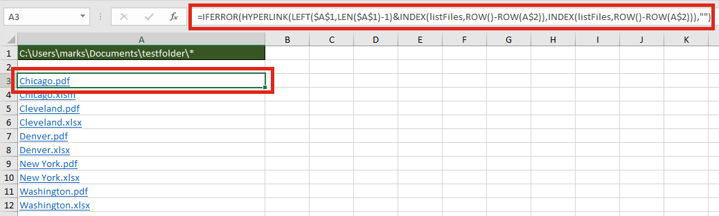
The formula in Cell A3 is:
=IFERROR(HYPERLINK(LEFT($A$1,LEN($A$1)-1)&INDEX(listFiles,ROW()-ROW(A$2)),
INDEX(listFiles,ROW()-ROW(A$2))),"")
Check if a specific file exists within a folder
It isn’t necessary to list all the files to find out if a file exists within the folder. The MATCH function will return the position of the file within the folder.
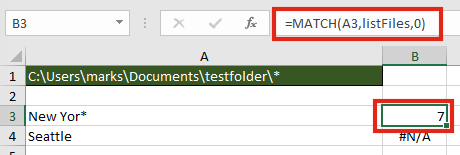
The formula in cell B3 is:
=MATCH(A3,listFiles,0)
In our example, a file which contains the text “New Yor*” exists, as the 7th file, therefore a 7 is returned. Cell B4 displays the #N/A error because “Seattle” does not exist in the folder.
Find the name of the next or previous file
The files returned are in alphabetical order, therefore it is possible to find the next or previous file using the INDEX / MATCH combination.
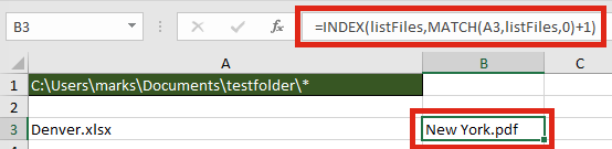
The next file after “Denver.xlsx” is “New York.pdf“. The formula in Cell B3 is:
=INDEX(listFiles,MATCH(A3,listFiles,0)+1)
Retrieve values from each file with INDIRECT
The INDIRECT function can construct a cell reference using text strings. Having retrieved the list of files in a folder, it would be possible to obtain values from those files.
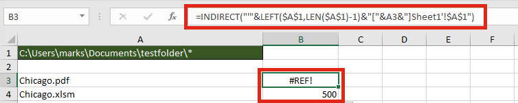
The formula in Cell B3 is:
=INDIRECT("'"&LEFT($A$1,LEN($A$1)-1)&"["&A3&"]Sheet1'!$A$1")
For INDIRECT to calculate correctly the file does need to be open, so this may be a significant flaw in this option.
Usage notes
When working with the FILES function there are a few things to be aware of:
- The file path and file name is not case sensitive
- Files are returned in alphabetical order
- Folders and hidden files are not returned by the function
- The workbook must be saved as a “.xlsm” file format
Further reading
There are variety of other Excel 4 functions available which still work in Excel. Check out this post to find out how to apply them and download the Excel 4 Macro functions reference guide.
If you decide to use a VBA method, check out this post.

About the author
Hey, I’m Mark, and I run Excel Off The Grid.
My parents tell me that at the age of 7 I declared I was going to become a qualified accountant. I was either psychic or had no imagination, as that is exactly what happened. However, it wasn’t until I was 35 that my journey really began.
In 2015, I started a new job, for which I was regularly working after 10pm. As a result, I rarely saw my children during the week. So, I started searching for the secrets to automating Excel. I discovered that by building a small number of simple tools, I could combine them together in different ways to automate nearly all my regular tasks. This meant I could work less hours (and I got pay raises!). Today, I teach these techniques to other professionals in our training program so they too can spend less time at work (and more time with their children and doing the things they love).
Do you need help adapting this post to your needs?
I’m guessing the examples in this post don’t exactly match your situation. We all use Excel differently, so it’s impossible to write a post that will meet everybody’s needs. By taking the time to understand the techniques and principles in this post (and elsewhere on this site), you should be able to adapt it to your needs.
But, if you’re still struggling you should:
- Read other blogs, or watch YouTube videos on the same topic. You will benefit much more by discovering your own solutions.
- Ask the ‘Excel Ninja’ in your office. It’s amazing what things other people know.
- Ask a question in a forum like Mr Excel, or the Microsoft Answers Community. Remember, the people on these forums are generally giving their time for free. So take care to craft your question, make sure it’s clear and concise. List all the things you’ve tried, and provide screenshots, code segments and example workbooks.
- Use Excel Rescue, who are my consultancy partner. They help by providing solutions to smaller Excel problems.
What next?
Don’t go yet, there is plenty more to learn on Excel Off The Grid. Check out the latest posts:
I am trying to clean up some existing code
Sheets("Control").Select
MyDir = Cells(2, 1)
CopySheet = Cells(6, 2)
MyFileName = Dir(MyDir & "wp*.xls")

' when the loop breaks, we know that any subsequent call to Dir implies
' that the file need to be added to the list
While MyFileName <> LastFileName
    MyFileName = Dir
Wend

MyFileName = Dir

While MyFileName <> ""
    Cells(LastRow + 1, 1) = MyFileName
    LastRow = LastRow + 1
    MyFileName = Dir
Wend
My question relates to how Dir returns results and if there are any guarantees on the order of results. When using Dir in a loop as above, the code implies that the resultant calls to Dir are ordered by name.
Unless Dir guarantees this, it’s a bug which needs to be fixed. The question, does Dir() make any guarantee on the order in which files are returned or is it implicit?
Solution
Based on @Frederic’s answer, this is the solution I came up with.
Using this quicksort algorithm in conjunction and a function that returns all files in a folder …
Dim allFiles As Variant
allFiles = GetFileList(MyDir & "wp*.xls")
If IsArray(allFiles) Then
    Call QuickSort(allFiles, LBound(allFiles), UBound(allFiles))
End If

Dim x As Integer
Dim lstFile As String
x = 1

' still need to loop through results to get lastFile
While lstFile <> LastFileName
    lstFile = allFiles(x)
    x = x + 1
Wend

For i = x To UBound(allFiles)
    MyFileName = allFiles(i)
    Cells(LastRow + 1, 1) = MyFileName
    LastRow = LastRow + 1
Next i
Options
- Subscribe to RSS Feed
- Mark Topic as New
- Mark Topic as Read
- Float this Topic for Current User
- Bookmark
- Subscribe
- Mute
- Printer Friendly Page

I have several workflows with multiple outputs, which I have generating on an Excel document. However, I haven’t found a rhyme or reasoning to the order of the sheets on my output document. Does anyone know of a way to control the output? In other words, a way to set my first output to the first tab in Excel, second output to the last tab in Excel, etc. Please let me know if this is something we can control in Alteryx. Thanks!
-
All forum topics -
Previous -
Next
9 REPLIES 9

Hi @mpollock
In Designer the output for the Excel sheets will be in alphabetical/numerical order. If you would like to amend this, the best way would be to add a numerical or alphabetical prefix to the field names to reflect the order you would like them to be output in.
Regards
Will
Hi Will, thanks for the reply! Are you saying they are in order based on the sheet name or actual data on the sheets? If it is by sheet name, I do not think the Designer is doing that. Attached is the order of my sheets for a workflow I have. Thanks! — Mike

One method I’ve used successfully to control the sheet order is to use a «Block Until Done» tool. That way, the sheets get added on in the order you want them (sample workflow attached).
If you have more than three sheets, you can just chain as many «Block Until Done» tools as you need.

Thanks for the reply Meteor! Only issue I see in the sample you sent is that each stream is coming from one input, not multiple like I have. In one workflow, I have 5 outputs from 2 inputs, while my other, I have 2 outputs from 8 input documents. The example I see below has 1 input generating all 3 outputs. If you have any other suggestions for my specific ask, please let me know. Thanks!
I see. One way to fix that would be to create a workbook with the sheets already created and in the order you want them, and then just have the multiple workflows overwrite the existing sheets. That will maintain the order regardless of which sheets get overwritten first.

Can you help me with any link or reference which will help me write the output to pre-saved template instead of creating output file.
Hi
Not quite true — I DO have a master excel sheet with the tabs created in the order I want — and the last tab written is placed into the middle of the other tabs.
In total I have 22 tabs / worksheets in my excel sheet in the order I want them
In my case I am inputting 1 excel file with 22 tabs, modifying quantity in those 22 tabs, then writing out for the same order.
On my outputs I do insert a BLOCK UNTIL DONE process
Terry

Hello,
The flow if we use the below pattern, we can define the tab when where we can keep the tab, based on your priorities. Adding the workfow sample.
Change the output path and run

If you have more than 3 keep 3rd out put to input as 2nd until block. As below:

![]()
Sorting data in Excel has been made quite easy with all the in-built options.
You can easily sort your data alphabetically, based on the value in the cells, or by cell and font color.
You can also do multi-level column sorting (i.e., sorting by column A and then by column B) as well as sorting rows (from left to right).
And if that was not enough, Excel also allows you to create your own custom lists and sort based on that too (how cool is that). So you can sort data based on shirt sizes (XL, L, M, S) or responses (strongly agree, agree, disagree) or intensity (high, medium, low)
Bottom line – there are just too many sorting options you have at your disposal when working with Excel.
And in this massive in-depth tutorial, I will show you all these sorting options and some cool examples where these can be useful.
Since this a huge tutorial with many topics, I am providing a table of content below. You can click on any of the topics and it will instantly take you there.
Accessing the Sorting Options in Excel
Since sorting is such a common thing needed when working with data, Excel provides a number of ways for you to access the sorting options.
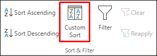
Sorting Buttons in the Ribbon
The fastest way to access sorting options is by using the sorting buttons in the ribbons.
When you click on the Data tab in the ribbon, you will see the ‘Sort & Filter’ options. The three buttons on the left in this group is for sorting the data.

The two small buttons allow you to sort your data as soon as you click on these.
![]()
For example, if you have a data set of names, you can just select the entire dataset and click on any of the two buttons to sort the data. The A to Z button sorts the data alphabetically lowest to highest and the Z to A button sorts the data alphabetically highest to lowest.
This buttons also work with numbers, dates or times.
Personally, I never use these buttons as these are limited in what these can do, and there are more chances of errors when using these. But in case you need a quick sort (where there are no blank cells in the dataset), these can be a fast way to do it.
Sorting Dialog Box
In the Data tab in the ribbon, there is another Sort button icon within the sorting group.

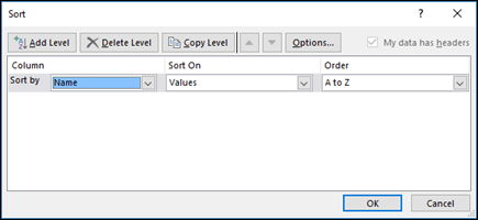
When you click this Sort button icon, it opens the sorting dialog box (something as shown below).
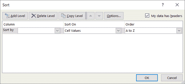
Sorting dialog is the most complete solution for sorting in Excel. All the sorting related options can be accessed through this dialog box.
All the other methods of using sorting options are limited and don’t offer full functionality.
This is the reason I always prefer using the dialog box when I have to sort in Excel.
A major reason for my preference is that there is very less chance of you going wrong when using the dialog box. Everything is well structured and marked (unlike buttons in the ribbon where you may get confused which one to use).
In this tutorial, you’ll find me mostly using the dialog box to sort the data. This is also because some of the things I cover in certain sections (such as multi-level sorting or sorting from left-to-right) can only be done using the dialog box.
Keyboard Shortcut – If you need to sort data often in Excel, I recommend you learn the keyboard shortcut to open the sort dialog box. It’s ALT + A + S + S
Sorting Options in the Filter Menu
If you have applied filters to your dataset, you can also find the sorting options along with the filter options. A filter can be applied by selecting any cell in the dataset, clicking on the Data tab and clicking in the Filter icon.
![]()
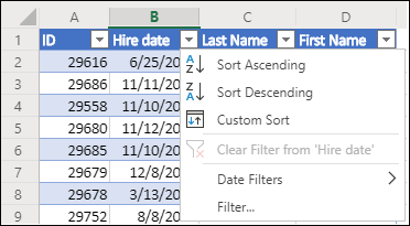
Suppose you have a dataset as shown below and you have the filter applied.

When you click on the filter icon for any column (it’s the small downward pointing triangle icon at the right of the column header cell), you’ll see some of the sorting options there as well.

Note that these sorting options change based on the data in the column. So if you have text, it will show you the option to sort from A to Z or Z to A, but if you have numbers, it will show you options to sort from largest to smallest or smallest to largest.
Right-click options
Apart from using the dialog box, using right-click is another method that I sometimes use (it’s also super fast as it only takes two clicks).
When you have a dataset that you want to sort, right-click on any cell and it will show you the sorting options.

Note that you see some options that you don’t see in the ribbon or in the Filter options. While there is the usual sort by value and custom sort option (which opens the Sort dialog box), you can also see options such as Put selected Cell color/Font color/Formatting icon on the top.
I find this option quite useful as it allows me to quickly get all the colored cells (or cells with a different font color) together at the top. I often have the monthly expense data that I go through and highlight some cells manually. I can then use this option to quickly get all these cells together at the top.
Now that I have covered all the ways to access sorting options in Excel, let’s see how to use these to sort data in different scenarios.
Also read: How to Undo Sort in Excel (Revert to Original)
Sorting Data in Excel (Text, Numbers, Dates)
Caveat: Most of the times, sorting works even when you select a single cell in the dataset. But in some cases, you may end up with issues (when you have blank cells/rows/columns in your dataset). When sorting data, it’s best to select the entire data set and then sort it – just to avoid any chance of issues.
Based on the type of data you have, you can use the sorting options in Excel.
Sorting by Text
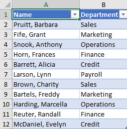
Suppose you have a dataset as shown below and you want to sort all these records based on the name of the student in alphabetical order.

Below are the steps to sort this text data in alphabetical order:
- Select the entire dataset
- Click the Data tab
- Click the Sort icon. This will open the Sort dialog box.

- In the Sort dialog box, make sure my data has headers is selected. In case your data doesn’t have headers, you can uncheck this.

- In the ‘Sort by’ drop-down, select ‘Name’
- In the ‘Sort On’ drop-down, make sure ‘Cell Values’ is selected
- In the Order drop-down, select A-Z
- Click OK.


The above steps would sort the entire dataset and give the result as shown below.

Why not just use the buttons in the ribbon?
The above method of sorting data in Excel may look like a lot of steps, as compared to just clicking the sort icon in the ribbon.
And this is true.
The above method is longer, but there is no chance of any error.
When you use the sort buttons in the ribbon, there are a few things that can go wrong (and this could be hard to spot when you have a large data set.
While I discuss the drawbacks of using the buttons later in this tutorial, let me quickly show you what can go wrong.
In the below example, since Excel cannot recognize that there is a header row, it sorts the entire dataset, including the header.
![]()
This issue is avoided with the sort dialog box as it explicitly gives you the option to specify whether your data has headers or not.
Since using the Sort dialog box eliminates chances of errors, I recommend you use it instead of all the other sorting methods in Excel
Sorting by Numbers
Now, I am assuming you have already gotten a hang of how text sorting works (covered above this section).
The other types of sorting (such as based on numbers or dates or color) is going to use almost the same steps with minor variations.
Suppose you have a dataset as shown below and you want to sort this data based on the marks scored by each student.

Below are the steps to sort this data based on numbers:
- Select the entire dataset
- Click the Data tab
- Click the Sort icon. This will open the Sort dialog box.
- In the Sort dialog box, make sure my data has headers is selected. In case your data doesn’t have headers, you can uncheck this.
- In the ‘Sort by’ drop-down, select ‘Name’
- In the ‘Sort On’ drop-down, make sure ‘Cell Values’ is selected
- In the Order drop-down, select ‘Largest to Smallest’
- Click OK.
The above steps would sort the entire dataset and give the result as shown below.

Sorting by Date/Time
While the date and time may look different, they are nothing but numbers.
For example, in Excel, the number 44196 would be the date value for 31 December 2020. You can format this number to look like a date, but in the backend in Excel, it still remains a number.
This also allows you to treat dates as numbers. So you can add 10 to a cell with date, and it will give you the number for the date 10 days later.
And the same goes for the time in Excel.
For example, the number 44196.125 represents 3 AM on 31st December 2020. While the integer part of the number represents a full day, the decimal part would give you the time.
And since both date and time are numbers, you can sort these like numbers.
Suppose you have a dataset as shown below and you want to sort this data based on the project submission date.

Below are the steps to sort this data based on the dates:
- Select the entire dataset
- Click the Data tab
- Click the Sort icon. This will open the Sort dialog box.
- In the Sort dialog box, make sure my data has headers is selected. In case your data doesn’t have headers, you can uncheck this.
- In the ‘Sort by’ drop-down, select ‘Submission Date’
- In the ‘Sort On’ drop-down, make sure ‘Cell Values’ is selected
- In the Order drop-down, select ‘Oldest to Newest’
- Click OK.
The above steps would sort the entire dataset and give the result as shown below.

Note that while date and time are numbers, Excel still recognized that these are different in the way it’s displayed. So when you sort by date, it shows ‘Oldest to Newest’ and ‘Newest to Oldest’ sorting criteria, but when you use numbers, it shows ‘Largest to Smallest’ or ‘Smallest to Largest’. Such small things that makes Excel an awesome spreadsheet tool (PS: Google Sheets doesn’t show so much detail, just the bland sort by A-Z or Z-A)
Sorting by Cell Color / Font Color
This option is amazing and I use it all the time (maybe a tad bit too much).
I often have data sets that I analyze manually and highlight cells while I am doing it. For example, I was going through a list of articles on this blog (which I have in an Excel sheet) and I highlighted the ones which I needed to improve.
And once I am done, I can quickly sort this data based on the cell colors. This helps me in getting all these highlighted cells/rows together at the top.
And to add to the awesomeness, you can sort based on multiple colors. So if I highlight cells with article names which need immediate attention in red and some which can be dealt with later with yellow, I can sort the data to show all the red rows first followed by the yellow.
If you’re interested in learning more, I recently wrote this article on sorting based on multiple colors. In this section, I will quickly show you how to sort based on one color only
Suppose you have a dataset as shown below and you want to sort by color and get all the red cells at the top.

Below are the steps to sort by color:
- Select the entire dataset
- Click the Data tab
- Click the Sort icon. This will open the Sort dialog box.
- In the Sort dialog box, make sure my data has headers is selected. In case your data doesn’t have headers, you can uncheck this.
- In the ‘Sort by’ drop-down, select ‘Submission Date’ (or whatever column where you have the colored cells).Since in this example we have colored cells in all the columns, you can choose any.
- In the ‘Sort On’ drop-down, select ‘Cell Color’.
- In the Order drop-down, select the color with which you want to sort. In case you have multiple cell colors in the dataset, it will show you all those colors here
- In the last drop-down, select ‘On Top’. This is where you specify whether you want the colored cells to be on the top of the dataset or at the bottom.
- Click OK.

The above steps would sort your dataset by color and you will get the result as shown below.

Just as we have sorted this data based on the cell color, you can also do it based on the font color and conditional formatting icon.
Multiple Level Data Sorting
In reality, datasets are rarely as simple as the one that I am using in this tutorial.
Yours may extend to thousands of rows and hundreds of columns.
And when you have datasets so big, there is also a need for more data slice and dice. Multiple level data sorting is one of the things you may need when you have a large data set.
Multiple level data sorting means that you can sort the dataset based on values in one column and then sort it again based on values in another column(s).
For example, suppose you have the dataset as shown below and you want to sort this data based on two criteria:
- The region
- The sales

The output of this sorting based on the above two criteria will give you a dataset as shown below.
In the above example, we have the data first sorted by the regions and then within each region, the data is further sorted by the sales value.
This quickly allows us to see which sales reps are doing great in each region or which ones are doing poorly.
Below are the steps to sort the data based on multiple columns:
- Select the entire data set that you want to sort.
- Click the Data tab.
- Click on the Sort Icon (the one shown below). This will open the Sort dialog box.
- In the Sort dialog box, make sure my data has headers is selected. In case your data doesn’t have headers, you can uncheck this.
- In the Sort Dialogue box, make the following selections
- Sort by (Column): Region (this is the first level of sorting)
- Sort On: Cell Values
- Order: A to Z
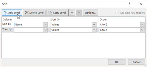
- Click on Add Level (this will add another level of sorting options).
- In the second level of sorting, make the following selections:
- Then by (Column): Sales
- Sort On: Values
- Order: Largest to Smallest
- Click OK


Pro Tip: The Sort dialog box has a feature to ‘Copy Level’. This quickly copies the selected sorting level and then you can easily modify it. It’s good to know feature and may end up saving you time in case you have to sort based on multiple columns.
Below is a video where I show how to do a multi-level sorting in Excel:
Sorting Based on a Custom List
While Excel already has some common sorting criteria (such as sorting alphabetically with text, smallest to largest or largest to smallest with numbers, oldest to newest or newest to oldest with dates), it may not be enough.
To give you an example, suppose I have the following dataset:

Now, if I sort it based on the region alphabetically, I have two options – A to Z or Z to A. Below is what I get when I sort this data alphabetically from A to Z using the region column.

But what if I want this sort order to be East, West, North, South?
You, of course, can rearrange the data after sorting, but that’s not the efficient way to do this.
The right way to do this would be using custom lists.
A custom list is a list that Excel allows you to create and then use just like the inbuilt lists (such as month names or weekday names). Once you have created a custom list, you can use it in features such as data sorting or fill handle.
Some example where custom lists can be useful include:
- Sorting the data based on region/city name
- Sorting based on T-shirt sizes – Small, Medium, Large, Extra Large
- Sorting based on survey responses – Strongly Agree, Agree, Neutral, Disagree
- Sorting based on probability – high, medium, low
The first step in trying to sort based on the custom criteria is to create the custom list.
Steps to create a custom list in Excel:
- Click the File tab

- Click on Options

- In the Excel Options Dialogue Box, select ‘Advanced’ from the list in the left pane.

- Within Advanced selected, scroll down and select ‘Edit Custom List’.

- In the Custom Lists dialogue box, type your criteria in the box titled List Entries. Type your criteria separated by comma (East, West, North, South) [you can also import your criteria if you have it listed].

- Click Add
- Click OK


Once you have completed the above steps, Excel will create and store a custom list that you can use for sorting data.
Note that the order of the items in the custom list is what determines how your list will be sorted.
When you create a custom list in one Excel workbook, it becomes available to all the workbooks in your system. So you only have to create it once and can reuse it in al workbooks.
Steps to sort using a custom list
Suppose you have the dataset as shown below and you want to sort it based on the regions (the sort order being East, West, North, and South)
Since we have already created a custom list, we can use it to sort our data.
Here are the steps to sort a dataset using a custom list:
- Select the entire dataset
- Click the Data tab
- Click the Sort icon. This will open the Sort dialog box.
- In the Sort dialog box, make sure my data has headers is selected. In case your data doesn’t have headers, you can uncheck this.
- In the ‘Sort by’ drop-down, select ‘Region’ (or whatever column where you have the colored cells)
- In the ‘Sort On’ drop-down, select ‘Cell Values’.
- In the Order drop-down, select ‘Custom List’. As soon as you click on it, it will open the Custom Lists dialog box.
- In the Custom Lists dialog box, select the custom list you have already created from the left pane.
- Click OK. Once you do this, you will see the custom sort criteria in the sort order drop-down field
- Click OK.


The above steps will sort your dataset based on the custom sort criteria.

Note: You don’t have to create a custom list before-hand to sort the data based on it. You can also create it while you’re in the Sort dialog box. When you click on Custom List (in step 7 above), it opens the custom list dialog box. You can create a custom list there as well.
Custom lists are not case sensitive. In case you want to do a case-sensitive sorting, refer to this example.
Also read: How to Sort by Length in Excel? Easy Formulas!
Sorting from Left to Right
While in most cases you’ll likely sort based on the column values, sometimes, you may also have a need to sort based on the row values.
For example, in the below dataset, I want to sort it based on the values in the Region row.

Although this type of data structure is not as common as the columnar data, I have still seen a lot of people working with this kind of construct.
Excel has an in-built functionality that allows you to sort from left to right.
Below are the steps to sort this data from left to right:
- Select the entire dataset (except the headers)
- Click the Data tab
- Click the Sort icon. This will open the Sort dialog box.
- In the Sort dialog box, click on Options.
- In the Sort Options dialog box, select ‘Sort left to right’

- Click OK.
- In the ‘Sort By’ drop-down, select Row 1. By doing this, we are specifying that the sort needs to be done based on the values in Row 1
- In the ‘Sort On’ drop-down, select ‘Cell Values’.
- In the Order drop-down, select A-Z (you can also use custom sort list if you want)
- Click OK.


The above steps would sort the data left to right based on Row 1 values.

Excel doesn’t recognize (or even allow you to specify) the headers when sorting from left to right. So you need to make sure your header cells are not selected when sorting the data. If you select headers cells as well, these will be sorted based on the value in it.
Note: Another way of sorting the data from right to left could be to transpose the data and get it in a columnar form. Once you have it, you can use any of the sorting methods covered so far. Once the sorting is done, you can then copy the resulting data and paste it as transposed data.
Below is a video where I show how to sort data from left to right in Excel
Case Sensitive Sorting in Excel
So far, in all the example above, the sorting has been case independent.
But what if you want to make the sorting case-sensitive.
Thankfully, Excel allows you to specify whether you want the sorting to be case-sensitive or not.
Note: While most of the times you don’t need to worry about case-sensitive sorting, this may be helpful when you get your data from a database such as Salesforce or you manually collate the data and have different people enter the same text in different cases. Having a case sensitive sort may help you keep all the records by the same person/database together.
Suppose you have a dataset as shown below and you want to sort this data based on the region column:

Below are the steps to sort data alphabetically as well as make it case sensitive:
- Select the entire dataset
- Click the Data tab
- Click the Sort icon. This will open the Sort dialog box.
- In the Sort dialog box, make sure my data has headers is selected. In case your data doesn’t have headers, you can uncheck this.
- Click the Options button
- In the Sort Options dialog box, check the ‘Case sensitive’ option
- Click OK.
- In the ‘Sort by’ drop-down, select ‘Region’
- In the ‘Sort On’ drop-down, select ‘Cell Values’.
- In the order drop-down, select A to Z
- Click OK.


The above steps would not only sort the data alphabetically based on the region, but also make it case-sensitive.
You’ll get the resulting data as shown below:

When you sort from A to Z, lower case text is placed above the upper case text.
Getting the Original Sort Order
Often when sorting data in Excel, you may want to go back to the earlier or the original sort order and start afresh,
While you can use the undo functionality in Excel (using Control Z) to go back one step at a time, it may be confusing if you have already done multiple things after sorting the data.
Also, undo works only till you have the workbook open, but when you save and close and it and open it later, you won’t be able to go back to the original sort order.
Here are two simple ways to make sure you don’t lose the original sort order and get it back even after sorting the data:
- Make a copy of the original dataset. This is something I recommend you do even if you don’t need the original sort order. You can have a workbook with all the data and then simply create a copy of the workbook and work on the copy. When I am working on critical datasets, I make a copy every day (with the date or version number as a part of the workbook name).
- Add a column with a series of number. This series of numbers get all mixed up when you sort the data, but in case you want to go back to the original data, you can sort based in this series of numbers.
In this section, let me quickly show you what mean by adding a series and using it to get original sort order back.
Suppose you have a dataset as shown below:

To make sure you have a way to get back this data after sorting it, add a helper column and have a series of numbers in it (as shown below).

Here is a tutorial with different ways to add a column with numbers quickly
When you have the helper column in place, make sure you include it while sorting this dataset.
Suppose I sort this data based on the region and end up getting the data as shown below:

Now, if I want to go back to the original dataset, I can simply sort this data again, but based on the helper column (from low to high).
Simple.. isn’t it?
In case you don’t want the helper column to show, you can either hide it or create a backup and then delete it.
Some Common Issues While Sorting Data in Excel
At the beginning of this article, I showed you different ways to sort data in Excel (including sort buttons in the ribbon, right-click options, filter option, and the sort dialog box).
And to reiterate, using the sort dialog box minimizes the chances or any issues or error that may arise.
Now, let me show you what can go wrong when you use the sort button from the ribbon (the ones shown below)
Not Identifying the Column Headers
Suppose you have a dataset as shown below:
This looks like a decently formatted data set with headers clearly formatted with cell color and bold font.
So when you sort this data based on the names (using the sort buttons in the ribbon), you would expect the header to remain at the top and rest of the data to get sorted.
But what happens when you do it – the header is also considered as normal data and gets sorted (as shown below).
![]()
While Excel is smart enough to recognize headers, in this example, it failed to do so. When using the sort icon buttons in the ribbon, there was no way for you to manually specify that this data has headers.
Note: This issue occurs when I have the dataset and I add and format the headers and sort it. Normally, Excel would be smart enough to identify that there are headers in a dataset (especially when the data type of the header and the data in the column is different). But in this case, it failed to do so when I added the header and sorted right away. If I save this workbook, close it and reopen it, Excel somehow manages to identify the first row and header.
While this may not be an issue in most cases, there is still a chance when you use the sort icons in the ribbon, Using a dialog box eliminates this issue as you can specify that you have headers.
Not Identifying Blank Rows/Columns
This sorting issue is a little more complex – and a lot more common than you would imagine.
Suppose you have a dataset as shown below. Note that row number 6 is hidden (and it’s a blank row).

Now, if I select any cell in the first four rows of the data (the ones above the hidden blank row) and sort this data using the sort icon buttons, it would only sort the first four records on the data set (row 2 to 5). Similarly, if I select any cell in the dataset below the hidden blank row, it will only sort the last seven rows.

And unless you’re looking for it specifically, you’re likely to miss this horrible error.
How to make sure you don’t end up making this sorting error?
To make sure you don’t fall prey to this issue, you need to check your dataset before sorting it.
Select the entire dataset before sorting the data.
You can do that by selecting any cell in the dataset and then using the keyboard shortcut – Control + A.
If there are blank rows/columns in your dataset, the entire dataset won’t get selected. You can identify this by quickly scanning the outline of the selection.
If you see that there is some data left outside the selection, you can manually select it.
To make sure this issue is avoided, it’s best to first unhide all hidden rows and columns and then proceed to sort the data by selecting the entire data set or by first deleting the blank rows.
Partial Sorting (Based on the Last Name)
Sometimes, you may have a dataset that you want to sort based on part of the text.
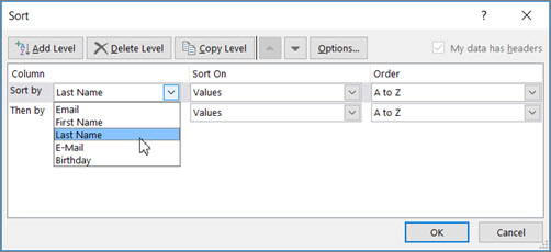
For example, suppose I have the dataset as shown below and I want to sort this data based on the last name.

To do this, I need to separate this data so that I have only the last names in one column. When I have it, I can use that column to sort the data.
Below is a formula that can give me the last name:
=RIGHT(B2,LEN(B2)-FIND(" ",B2))
This will give you a result as shown below.

Now you can use the Last Name column to sort this data.
Once done, you can delete the last name column or hide it.
Note that the above formula works when you have names that has first and last name only and have no double spaces in between. In case you have names data that is different, you will have to adjust the formula. You can also use Text to Column to quickly split the names based on space character as the delimiter.
This is just one example of sorting based on partial data. Other examples may include sorting based on cities in an address or employee ID based on department codes.
Also, in case the text based on which you need to sort is at the beginning of the text, you can use the normal sort feature only.
Other Sorting Examples (Using Formula and VBA)
So far in this tutorial, I have covered the examples where we have used the in-built sorting functionality in Excel.
Automatically Sorting Using a Formula
When you use the in-built sort functionality and then make any change in the data set, you need to sort it again. The sort functionality is not dynamic.
In case you want to get a dataset that sorts automatically whenever there is any change, you can use the formulas to do it.
Note that to do this, you need to keep the original dataset and the sorted dataset separate (as shown below)

I have a detailed tutorial where I cover how to sort alphabetically using formulas. It shows two methods to do this – using helper columns and using an array formula.
Excel has also introduced the SORT dynamic array formula which can easily do this (without helper column or a complicated array formula). But since this is quite new, you may not have access to it in your version of Excel.
Sorting Using VBA
And finally, if you want to bypass all the sorting dialog box or other sorting options, you can use VBA to sort your data.
In the below example, I have a dataset that sorts the data when I double click on the column header. This makes it easy to sort and can be used in dashboards to make it more user-friendly.
Here is a detailed tutorial where I cover how to sort data using VBA and create something as shown above.
I have tried to cover a lot of examples to show you different ways you can sort data in Excel and all the things you need to keep in mind when doing it.
Hope you found this tutorial useful.
You May Also Like the following Excel Tutorials:
- Search and Highlight Data Using Conditional Formatting
- How to Sort Worksheets in Excel using VBA
- How to Create a Data Entry Form in Excel
- How to Compare Two Columns in Excel
- Excel TRIM Function to Remove Spaces and Clean Data
- Flip Data in Excel | Reverse Order of Data in Column/Row
- How to Shuffle a List of Items/Names in Excel? 2 Easy Formulas!