
Abstract: This is the first tutorial in a series designed to get you acquainted and comfortable using Excel and its built-in data mash-up and analysis features. These tutorials build and refine an Excel workbook from scratch, build a data model, then create amazing interactive reports using Power View. The tutorials are designed to demonstrate Microsoft Business Intelligence features and capabilities in Excel, PivotTables, Power Pivot, and Power View.
Note: This article describes data models in Excel 2013. However, the same data modeling and Power Pivot features introduced in Excel 2013 also apply to Excel 2016.
In these tutorials you learn how to import and explore data in Excel, build and refine a data model using Power Pivot, and create interactive reports with Power View that you can publish, protect, and share.
The tutorials in this series are the following:
-
Import Data into Excel 2013, and Create a Data Model
-
Extend Data Model relationships using Excel, Power Pivot, and DAX
-
Create Map-based Power View Reports
-
Incorporate Internet Data, and Set Power View Report Defaults
-
Power Pivot Help
-
Create Amazing Power View Reports — Part 2
In this tutorial, you start with a blank Excel workbook.
The sections in this tutorial are the following:
-
Import data from a database
-
Import data from a spreadsheet
-
Import data using copy and paste
-
Create a relationship between imported data
-
Checkpoint and Quiz
At the end of this tutorial is a quiz you can take to test your learning.
This tutorial series uses data describing Olympic Medals, hosting countries, and various Olympic sporting events. We suggest you go through each tutorial in order. Also, tutorials use Excel 2013 with Power Pivot enabled. For more information on Excel 2013, click here. For guidance on enabling Power Pivot, click here.
Import data from a database
We start this tutorial with a blank workbook. The goal in this section is to connect to an external data source, and import that data into Excel for further analysis.
Let’s start by downloading some data from the Internet. The data describes Olympic Medals, and is a Microsoft Access database.
-
Click the following links to download files we use during this tutorial series. Download each of the four files to a location that’s easily accessible, such as Downloads or My Documents, or to a new folder you create:
> OlympicMedals.accdb Access database
> OlympicSports.xlsx Excel workbook
> Population.xlsx Excel workbook
> DiscImage_table.xlsx Excel workbook -
In Excel 2013, open a blank workbook.
-
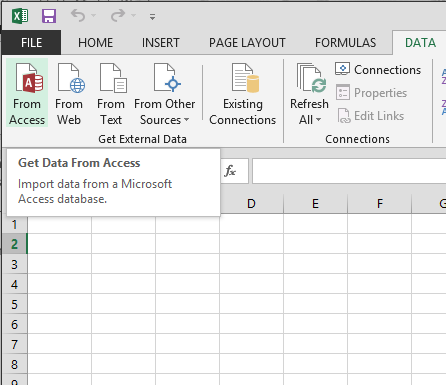
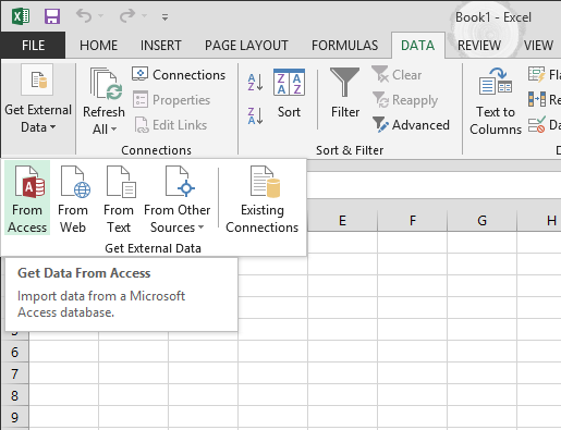
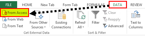
Click DATA > Get External Data > From Access. The ribbon adjusts dynamically based on the width of your workbook, so the commands on your ribbon may look slightly different from the following screens. The first screen shows the ribbon when a workbook is wide, the second image shows a workbook that has been resized to take up only a portion of the screen.

-
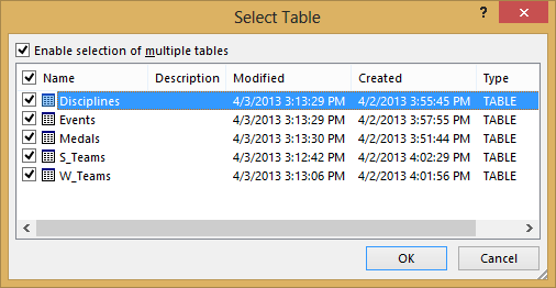
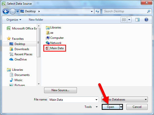
Select the OlympicMedals.accdb file you downloaded and click Open. The following Select Table window appears, displaying the tables found in the database. Tables in a database are similar to worksheets or tables in Excel. Check the Enable selection of multiple tables box, and select all the tables. Then click OK.
-
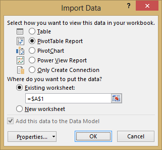
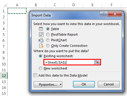
The Import Data window appears.
Note: Notice the checkbox at the bottom of the window that allows you to Add this data to the Data Model, shown in the following screen. A Data Model is created automatically when you import or work with two or more tables simultaneously. A Data Model integrates the tables, enabling extensive analysis using PivotTables, Power Pivot, and Power View. When you import tables from a database, the existing database relationships between those tables is used to create the Data Model in Excel. The Data Model is transparent in Excel, but you can view and modify it directly using the Power Pivot add-in. The Data Model is discussed in more detail later in this tutorial.
Select the PivotTable Report option, which imports the tables into Excel and prepares a PivotTable for analyzing the imported tables, and click OK.
-
Once the data is imported, a PivotTable is created using the imported tables.
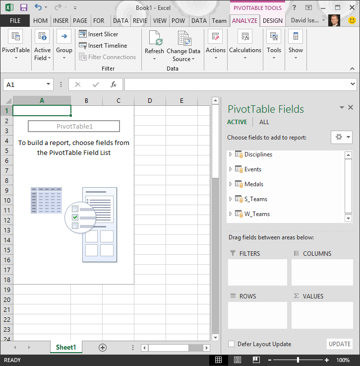
With the data imported into Excel, and the Data Model automatically created, you’re ready to explore the data.
Explore data using a PivotTable
Exploring imported data is easy using a PivotTable. In a PivotTable, you drag fields (similar to columns in Excel) from tables (like the tables you just imported from the Access database) into different areas of the PivotTable to adjust how it presents your data. A PivotTable has four areas: FILTERS, COLUMNS, ROWS, and VALUES.
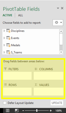
It might take some experimenting to determine which area a field should be dragged to. You can drag as many or few fields from your tables as you like, until the PivotTable presents your data how you want to see it. Feel free to explore by dragging fields into different areas of the PivotTable; the underlying data is not affected when you arrange fields in a PivotTable.
Let’s explore the Olympic Medals data in the PivotTable, starting with Olympic medalists organized by discipline, medal type, and the athlete’s country or region.
-
In PivotTable Fields, expand the Medals table by clicking the arrow beside it. Find the NOC_CountryRegion field in the expanded Medals table, and drag it to the COLUMNS area. NOC stands for National Olympic Committees, which is the organizational unit for a country or region.
-
Next, from the Disciplines table, drag Discipline to the ROWS area.
-
Let’s filter Disciplines to display only five sports: Archery, Diving, Fencing, Figure Skating, and Speed Skating. You can do this from within the PivotTable Fields area, or from the Row Labels filter in the PivotTable itself.
-
Click anywhere in the PivotTable to ensure the Excel PivotTable is selected. In the PivotTable Fields list, where the Disciplines table is expanded, hover over its Discipline field and a dropdown arrow appears to the right of the field. Click the dropdown, click (Select All)to remove all selections, then scroll down and select Archery, Diving, Fencing, Figure Skating, and Speed Skating. Click OK.
-
Or, in the Row Labels section of the PivotTable, click the dropdown next to Row Labels in the PivotTable, click (Select All) to remove all selections, then scroll down and select Archery, Diving, Fencing, Figure Skating, and Speed Skating. Click OK.
-
-
In PivotTable Fields, from the Medals table, drag Medal to the VALUES area. Since Values must be numeric, Excel automatically changes Medal to Count of Medal.
-
From the Medals table, select Medal again and drag it into the FILTERS area.
-
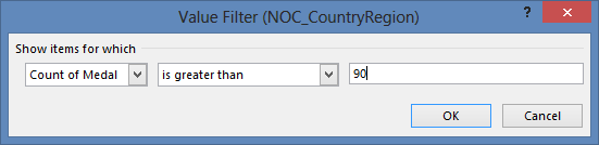
Let’s filter the PivotTable to display only those countries or regions with more than 90 total medals. Here’s how.
-
In the PivotTable, click the dropdown to the right of Column Labels.
-
Select Value Filters and select Greater Than….
-
Type 90 in the last field (on the right). Click OK.
-
Your PivotTable looks like the following screen.
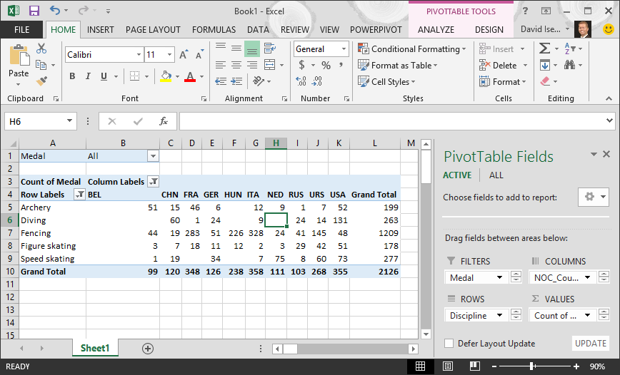
With little effort, you now have a basic PivotTable that includes fields from three different tables. What made this task so simple were the pre-existing relationships among the tables. Because table relationships existed in the source database, and because you imported all the tables in a single operation, Excel could recreate those table relationships in its Data Model.
But what if your data originates from different sources, or is imported at a later time? Typically, you can create relationships with new data based on matching columns. In the next step, you import additional tables, and learn how to create new relationships.
Import data from a spreadsheet
Now let’s import data from another source, this time from an existing workbook, then specify the relationships between our existing data and the new data. Relationships let you analyze collections of data in Excel, and create interesting and immersive visualizations from the data you import.
Let’s start by creating a blank worksheet, then import data from an Excel workbook.
-
Insert a new Excel worksheet, and name it Sports.
-
Browse to the folder that contains the downloaded sample data files, and open OlympicSports.xlsx.
-
Select and copy the data in Sheet1. If you select a cell with data, such as cell A1, you can press Ctrl + A to select all adjacent data. Close the OlympicSports.xlsx workbook.
-
On the Sports worksheet, place your cursor in cell A1 and paste the data.
-
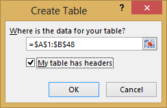
With the data still highlighted, press Ctrl + T to format the data as a table. You can also format the data as a table from the ribbon by selecting HOME > Format as Table. Since the data has headers, select My table has headers in the Create Table window that appears, as shown here.
Formatting the data as a table has many advantages. You can assign a name to a table, which makes it easy to identify. You can also establish relationships between tables, enabling exploration and analysis in PivotTables, Power Pivot, and Power View.
-
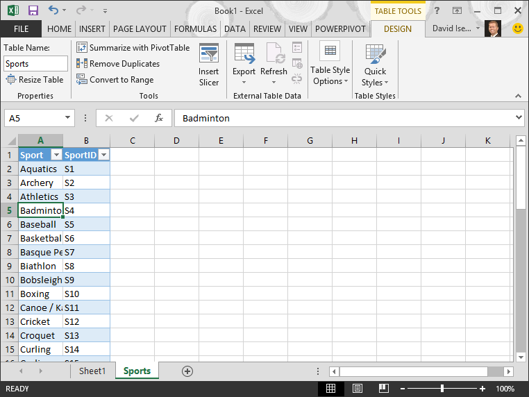
Name the table. In TABLE TOOLS > DESIGN > Properties, locate the Table Name field and type Sports. The workbook looks like the following screen.
-
Save the workbook.
Import data using copy and paste
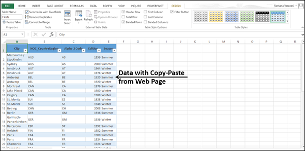
Now that we’ve imported data from an Excel workbook, let’s import data from a table we find on a web page, or any other source from which we can copy and paste into Excel. In the following steps, you add the Olympic host cities from a table.
-
Insert a new Excel worksheet, and name it Hosts.
-
Select and copy the following table, including the table headers.
|
City |
NOC_CountryRegion |
Alpha-2 Code |
Edition |
Season |
|
Melbourne / Stockholm |
AUS |
AS |
1956 |
Summer |
|
Sydney |
AUS |
AS |
2000 |
Summer |
|
Innsbruck |
AUT |
AT |
1964 |
Winter |
|
Innsbruck |
AUT |
AT |
1976 |
Winter |
|
Antwerp |
BEL |
BE |
1920 |
Summer |
|
Antwerp |
BEL |
BE |
1920 |
Winter |
|
Montreal |
CAN |
CA |
1976 |
Summer |
|
Lake Placid |
CAN |
CA |
1980 |
Winter |
|
Calgary |
CAN |
CA |
1988 |
Winter |
|
St. Moritz |
SUI |
SZ |
1928 |
Winter |
|
St. Moritz |
SUI |
SZ |
1948 |
Winter |
|
Beijing |
CHN |
CH |
2008 |
Summer |
|
Berlin |
GER |
GM |
1936 |
Summer |
|
Garmisch-Partenkirchen |
GER |
GM |
1936 |
Winter |
|
Barcelona |
ESP |
SP |
1992 |
Summer |
|
Helsinki |
FIN |
FI |
1952 |
Summer |
|
Paris |
FRA |
FR |
1900 |
Summer |
|
Paris |
FRA |
FR |
1924 |
Summer |
|
Chamonix |
FRA |
FR |
1924 |
Winter |
|
Grenoble |
FRA |
FR |
1968 |
Winter |
|
Albertville |
FRA |
FR |
1992 |
Winter |
|
London |
GBR |
UK |
1908 |
Summer |
|
London |
GBR |
UK |
1908 |
Winter |
|
London |
GBR |
UK |
1948 |
Summer |
|
Munich |
GER |
DE |
1972 |
Summer |
|
Athens |
GRC |
GR |
2004 |
Summer |
|
Cortina d’Ampezzo |
ITA |
IT |
1956 |
Winter |
|
Rome |
ITA |
IT |
1960 |
Summer |
|
Turin |
ITA |
IT |
2006 |
Winter |
|
Tokyo |
JPN |
JA |
1964 |
Summer |
|
Sapporo |
JPN |
JA |
1972 |
Winter |
|
Nagano |
JPN |
JA |
1998 |
Winter |
|
Seoul |
KOR |
KS |
1988 |
Summer |
|
Mexico |
MEX |
MX |
1968 |
Summer |
|
Amsterdam |
NED |
NL |
1928 |
Summer |
|
Oslo |
NOR |
NO |
1952 |
Winter |
|
Lillehammer |
NOR |
NO |
1994 |
Winter |
|
Stockholm |
SWE |
SW |
1912 |
Summer |
|
St Louis |
USA |
US |
1904 |
Summer |
|
Los Angeles |
USA |
US |
1932 |
Summer |
|
Lake Placid |
USA |
US |
1932 |
Winter |
|
Squaw Valley |
USA |
US |
1960 |
Winter |
|
Moscow |
URS |
RU |
1980 |
Summer |
|
Los Angeles |
USA |
US |
1984 |
Summer |
|
Atlanta |
USA |
US |
1996 |
Summer |
|
Salt Lake City |
USA |
US |
2002 |
Winter |
|
Sarajevo |
YUG |
YU |
1984 |
Winter |
-
In Excel, place your cursor in cell A1 of the Hosts worksheet and paste the data.
-
Format the data as a table. As described earlier in this tutorial, you press Ctrl + T to format the data as a table, or from HOME > Format as Table. Since the data has headers, select My table has headers in the Create Table window that appears.
-
Name the table. In TABLE TOOLS > DESIGN > Properties locate the Table Name field, and type Hosts.
-
Select the Edition column, and from the HOME tab, format it as Number with 0 decimal places.
-
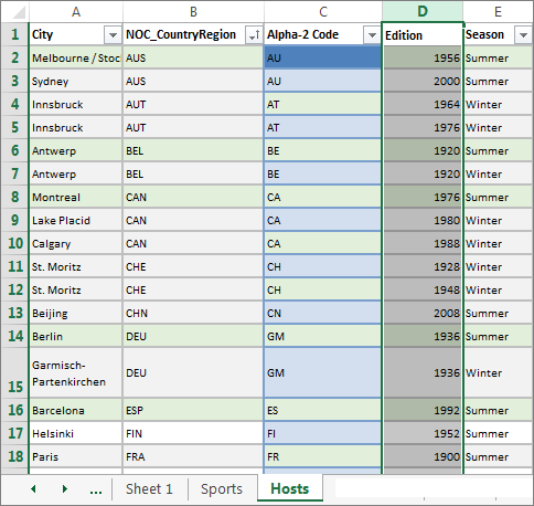
Save the workbook. Your workbook looks like the following screen.
Now that you have an Excel workbook with tables, you can create relationships between them. Creating relationships between tables lets you mash up the data from the two tables.
Create a relationship between imported data
You can immediately begin using fields in your PivotTable from the imported tables. If Excel can’t determine how to incorporate a field into the PivotTable, a relationship must be established with the existing Data Model. In the following steps, you learn how to create a relationship between data you imported from different sources.
-
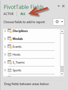
On Sheet1, at the top ofPivotTable Fields, clickAll to view the complete list of available tables, as shown in the following screen.
-
Scroll through the list to see the new tables you just added.
-
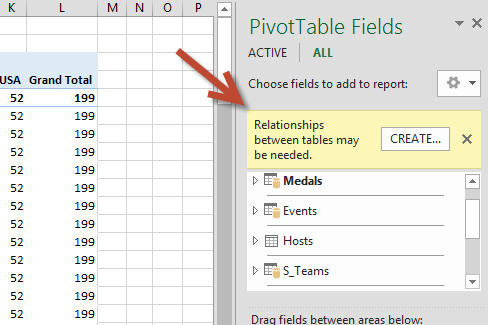
Expand Sports and select Sport to add it to the PivotTable. Notice that Excel prompts you to create a relationship, as seen in the following screen.
This notification occurs because you used fields from a table that’s not part of the underlying Data Model. One way to add a table to the Data Model is to create a relationship to a table that’s already in the Data Model. To create the relationship, one of the tables must have a column of unique, non-repeated, values. In the sample data, the Disciplines table imported from the database contains a field with sports codes, called SportID. Those same sports codes are present as a field in the Excel data we imported. Let’s create the relationship.
-
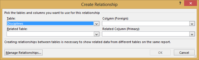
Click CREATE… in the highlighted PivotTable Fields area to open the Create Relationship dialog, as shown in the following screen.
-
In Table, choose Disciplines from the drop down list.
-
In Column (Foreign), choose SportID.
-
In Related Table, choose Sports.
-
In Related Column (Primary), choose SportID.
-
Click OK.
The PivotTable changes to reflect the new relationship. But the PivotTable doesn’t look right quite yet, because of the ordering of fields in the ROWS area. Discipline is a subcategory of a given sport, but since we arranged Discipline above Sport in the ROWS area, it’s not organized properly. The following screen shows this unwanted ordering.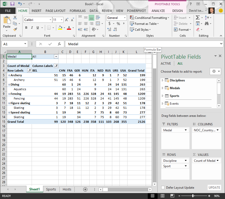
-
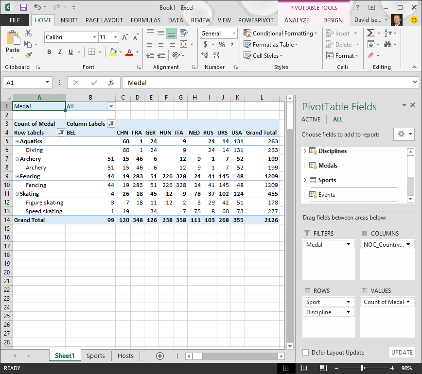
In the ROWS area, move Sport above Discipline. That’s much better, and the PivotTable displays the data how you want to see it, as shown in the following screen.
Behind the scenes, Excel is building a Data Model that can be used throughout the workbook, in any PivotTable, PivotChart, in Power Pivot, or any Power View report. Table relationships are the basis of a Data Model, and what determine navigation and calculation paths.
In the next tutorial, Extend Data Model relationships using Excel 2013, Power Pivot, and DAX, you build on what you learned here, and step through extending the Data Model using a powerful and visual Excel add-in called Power Pivot. You also learn how to calculate columns in a table, and use that calculated column so that an otherwise unrelated table can be added to your Data Model.
Checkpoint and Quiz
Review What You’ve Learned
You now have an Excel workbook that includes a PivotTable accessing data in multiple tables, several of which you imported separately. You learned to import from a database, from another Excel workbook, and from copying data and pasting it into Excel.
To make the data work together, you had to create a table relationship that Excel used to correlate the rows. You also learned that having columns in one table that correlate to data in another table is essential for creating relationships, and for looking up related rows.
You’re ready for the next tutorial in this series. Here’s a link:
Extend Data Model relationships using Excel 2013, Power Pivot, and DAX
QUIZ
Want to see how well you remember what you learned? Here’s your chance. The following quiz highlights features, capabilities, or requirements you learned about in this tutorial. At the bottom of the page, you’ll find the answers. Good luck!
Question 1: Why is it important to convert imported data into tables?
A: You don’t have to convert them into tables, because all imported data is automatically turned into tables.
B: If you convert imported data into tables, they will be excluded from the Data Model. Only when they’re excluded from the Data Model are they available in PivotTables, Power Pivot, and Power View.
C: If you convert imported data into tables, they can be included in the Data Model, and be made available to PivotTables, Power Pivot, and Power View.
D: You cannot convert imported data into tables.
Question 2: Which of the following data sources can you import into Excel, and include in the Data Model?
A: Access Databases, and many other databases as well.
B: Existing Excel files.
C: Anything you can copy and paste into Excel and format as a table, including data tables in websites, documents, or anything else that can be pasted into Excel.
D: All of the above
Question 3: In a PivotTable, what happens when you reorder fields in the four PivotTable Fields areas?
A: Nothing – you cannot reorder fields once you place them in the PivotTable Fields areas.
B: The PivotTable format is changed to reflect the layout, but underlying data is unaffected.
C: The PivotTable format is changed to reflect the layout, and all underlying data is permanently changed.
D: The underlying data is changed, resulting in new data sets.
Question 4: When creating a relationship between tables, what is required?
A: Neither table can have any column that contains unique, non-repeated values.
B: One table must not be part of the Excel workbook.
C: The columns must not be converted to tables.
D: None of the above is correct.
Quiz Answers
-
Correct answer: C
-
Correct answer: D
-
Correct answer: B
-
Correct answer: D
Notes: Data and images in this tutorial series are based on the following:
-
Olympics Dataset from Guardian News & Media Ltd.
-
Flag images from CIA Factbook (cia.gov)
-
Population data from The World Bank (worldbank.org)
-
Olympic Sport Pictograms by Thadius856 and Parutakupiu
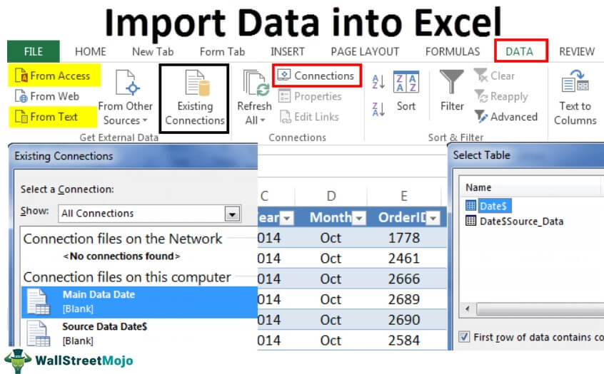
How to Import Data in Excel?
Importing the data from another file or another source file is often required in Excel. For example, sometimes people need data directly from very complicated servers, and sometimes we may need to import data from a text file or even from an Excel workbook.
If you are new to Excel data importing, then in this article, we will take a tour of importing data from text files, different Excel workbooks, and MS Access. Follow this article to learn the process involved in importing the data.
Table of contents
- How to Import Data in Excel?
- #1 – Import Data from Another Excel Workbook
- #2 – Import Data from MS Access to Excel
- #3 – Import Data from Text File to Excel
- Things to Remember
- Recommended Articles
#1 – Import Data from Another Excel Workbook
You can download this Import Data Excel Template here – Import Data Excel Template
Let us start.
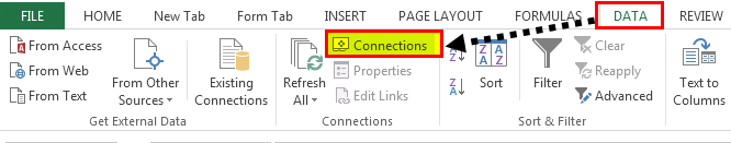
- First, we must go to the DATA tab. Then, under the DATA tab, click on Connections.

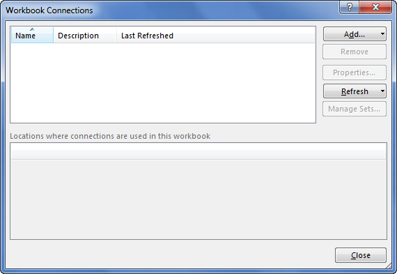
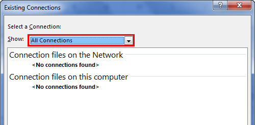
- As soon as we click on Connections, we may see the below window separately.

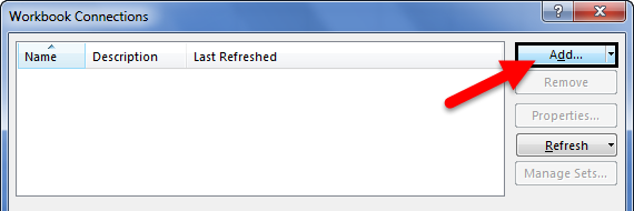
- Now, click on Add.

- It will open up a new window. In the below window, select All Connections.

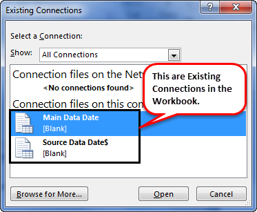
- If there are any connections in this workbook, it will show what those connections are here.

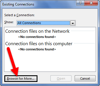
- Since we are connecting to a new workbook, click on Browse for more.

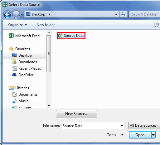
- In the below window, browse the file location. Then, click on Open.

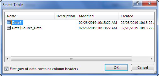
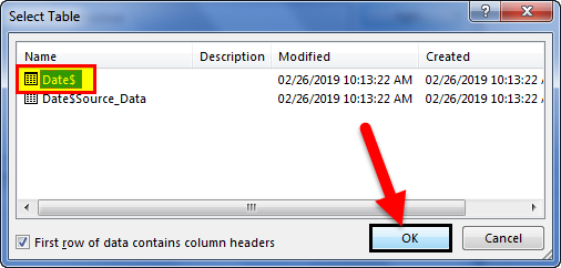
- After clicking on Open, it shows the below window.

- Here, we need to select the required table to be imported to this workbook. Select the table and click on OK.
After clicking on OK, close the Workbook Connection window.
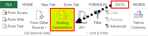
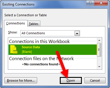
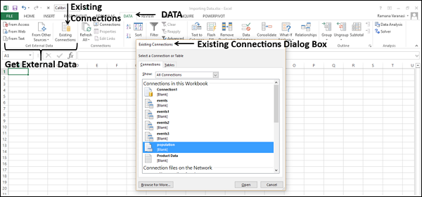
- Then, go to Existing Connections under the DATA tab.

- Here, we will see all the existing connections. Select the connection we have just made and click on Open.

- Once we click on Open, it will ask us where to import the data. First, we need to select the cell reference here. Then, click on the OK button.

- It will import the data from the selected or connected workbook.

Like this, we can connect to the other workbook and import the data.
#2 – Import Data from MS Access to Excel
MS Access is the main platform to store the data safely. We can import the data directly from the MS Access File itself whenever the data is required.
Step 1: Go to the “DATA” ribbon in excelThe ribbon is an element of the UI (User Interface) which is seen as a strip that consists of buttons or tabs; it is available at the top of the excel sheet. This option was first introduced in the Microsoft Excel 2007.read more and select “From Access.“
Step 2: Now, it will ask us to locate the desired file. Select the desired file path. Then, click on “Open.”
Step 3: Now, it will ask us to select the desired destination cell where we want to import the data. Then, click on “OK.”
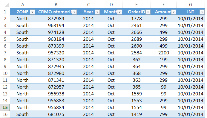
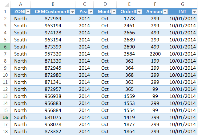
Step 4: It will import the data from access to the A1 cell in Excel.
#3 – Import Data from Text File to Excel
In almost all the corporations, whenever we ask for the data from the IT team, they will write a query and get the file in TEXT format. But unfortunately, TEXT file data is not the ready format to use in Excel; we need to make some modifications to work on it.
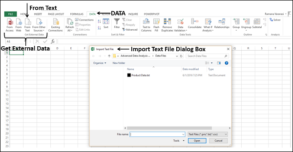
Step 1: Go to the “DATA” tab and click on “From Text.”

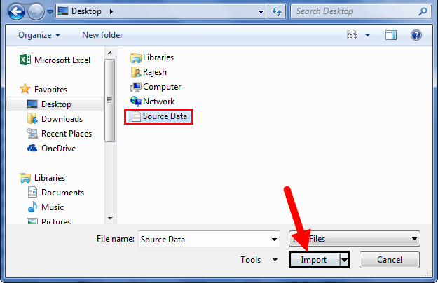
Step 2: Now, it will ask us to choose the file location on the computer or laptop. Select the targeted file, then click on “Import.”
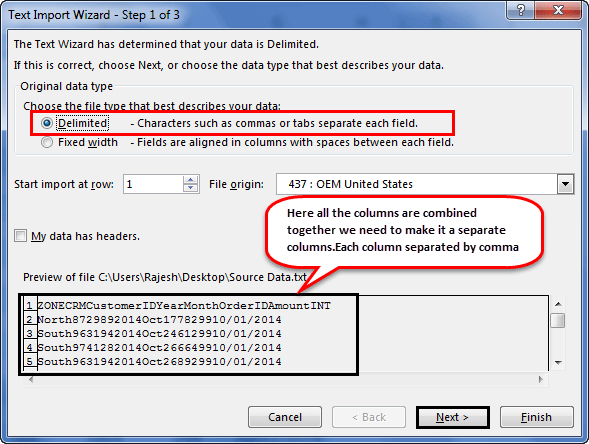
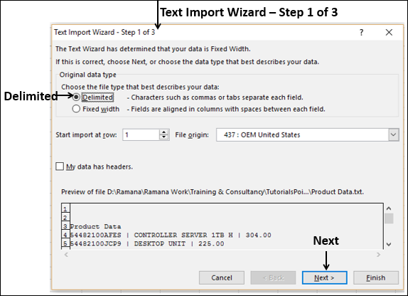
Step 3: It will open up a “Text Import Wizard.”
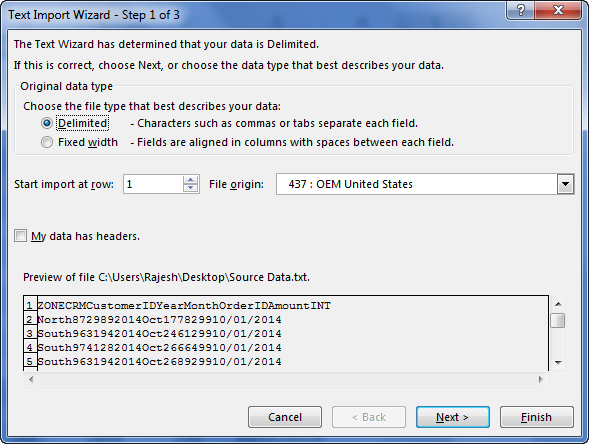
Step 4: By selecting the “Delimited,” click on “Next.”
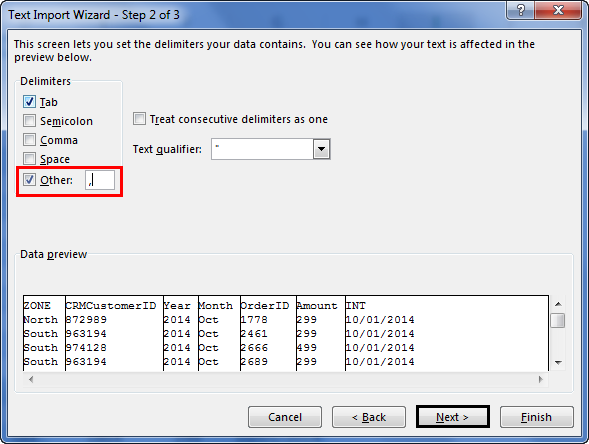
Step 5: In the next window, select the other and mention comma (,) because, in the text file, each column is separated by a comma (,). Then click on “Next.”
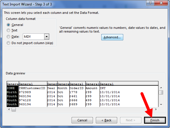
Step 6: In the next window, click on “Finish.”
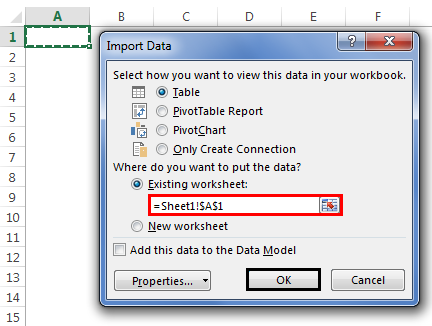
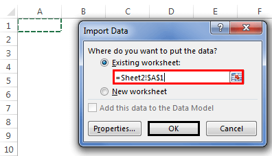
Step 7: Now, it will ask us to select the desired destination cell where we want to import the data. Select the cell and click on “OK.”
Step 8: It will import the data from the text file to the A1 cell in Excel.
Things to Remember
- If there are many tables, we must specify which table data we need to import.
- If we want the data in the current worksheet, we need to select the desired cell. Else, if we need data in a new worksheet, we must choose the new worksheet as the option.
- We need to separate the column in the TEXT file by identifying the common column separators.
Recommended Articles
This article is a guide to Import Data in Excel. Here, we discuss how to import data from 1) Excel Workbook, 2) MS Access, 3) Text File, practical examples, and a downloadable Excel template. You may learn more about Excel from the following articles: –
- KPI Dashboard in Excel
- Insert Image in Excel Cell
- How to Insert New Worksheet In Excel?
- Create a Dashboard in Excel
- Page Numbers in Excel
Excel can import and export many different file types aside from the standard .xslx format. If your data is shared between other programs, like a database, you may need to save data as a different file type or bring in files of a different file type.
Export Data
When you have data that needs to be transferred to another system, export it from Excel in a format that can be interpreted by other programs, such as a text or CSV file.
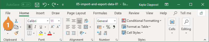
- Click the File tab.

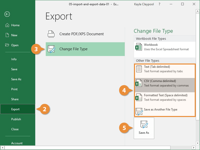
- At the left, click Export.
- Click the Change File Type.
- Under Other File Types, select a file type.
- Text (Tab delimited): The cell data will be separated by a tab.
- CSV (Comma delimited): The cell data will be separated by a comma.
- Formatted Text (space delimited): The cell data will be separated by a space.
- Save as Another File Type: Select a different file type when the Save As dialog box appears.
The file type you select will depend on what type of file is required by the program that will consume the exported data.
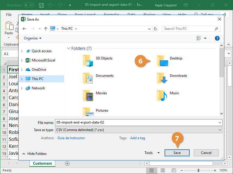
- Click Save As.

- Specify where you want to save the file.
- Click Save.
A dialog box appears stating that some of the workbook features may be lost.
- Click Yes.
Import Data
Excel can import data from external data sources including other files, databases, or web pages.
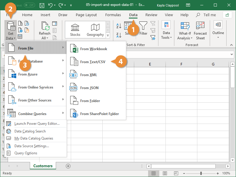
- Click the Data tab on the Ribbon..
- Click the Get Data button.
Some data sources may require special security access, and the connection process can often be very complex. Enlist the help of your organization’s technical support staff for assistance.
- Select From File.
- Select From Text/CSV.
If you have data to import from Access, the web, or another source, select one of those options in the Get External Data group instead.
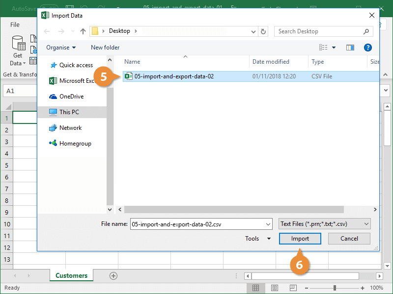
- Select the file you want to import.
- Click Import.
If, while importing external data, a security notice appears saying that it is connecting to an external source that may not be safe, click OK.
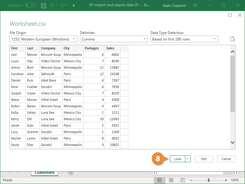
- Verify the preview looks correct.
Because we’ve specified the data is separated by commas, the delimiter is already set. If you need to change it, it can be done from this menu.
- Click Load.

FREE Quick Reference
Click to Download
Free to distribute with our compliments; we hope you will consider our paid training.
You might have to use data from various sources for analysis. In Excel, you can import data from different data sources. Some of the data sources are as follows −
- Microsoft Access Database
- Web Page
- Text File
- SQL Server Table
- SQL Server Analysis Cube
- XML File
You can import any number of tables simultaneously from a database.
Importing Data from Microsoft Access Database
We will learn how to import data from MS Access database. Follow the steps given below −
Step 1 − Open a new blank workbook in Excel.
Step 2 − Click the DATA tab on the Ribbon.
Step 3 − Click From Access in the Get External Data group. The Select Data Source dialog box appears.
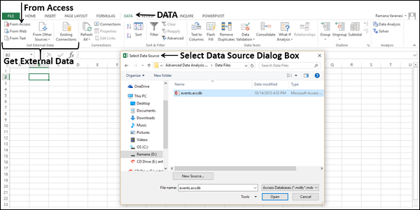
Step 4 − Select the Access database file that you want to import. Access database files will have the extension .accdb.
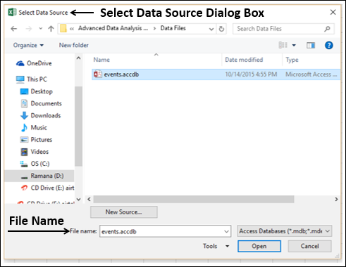
The Select Table dialog box appears displaying the tables found in the Access database. You can either import all the tables in the database at once or import only the selected tables based on your data analysis needs.
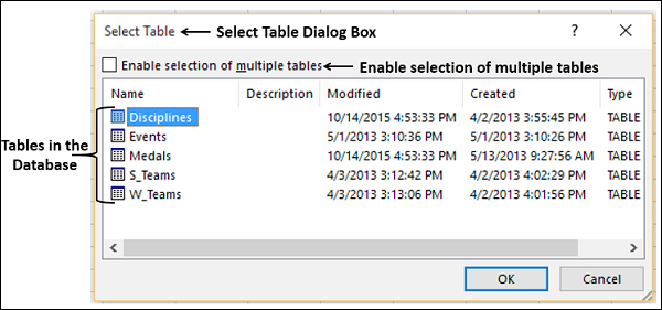
Step 5 − Select the Enable selection of multiple tables box and select all the tables.
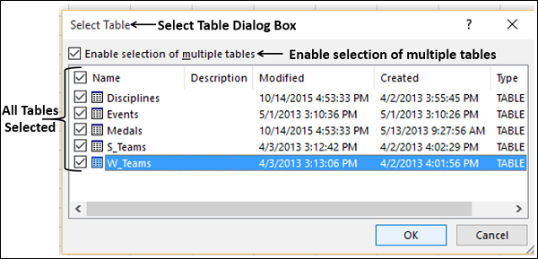
Step 6 − Click OK. The Import Data dialog box appears.
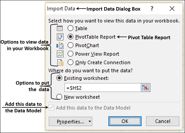
As you observe, you have the following options to view the data you are importing in your workbook −
- Table
- PivotTable Report
- PivotChart
- Power View Report
You also have an option — only create connection. Further, PivotTable Report is selected by default.
Excel also gives you the options to put the data in your workbook −
- Existing worksheet
- New worksheet
You will find another check box that is selected and disabled – Add this data to the Data Model. Whenever you import data tables into your workbook, they are automatically added to the Data Model in your workbook. You will learn more about the Data Model in later chapters.
You can try each one of the options to view the data you are importing, and check how the data appears in your workbook −
-
If you select Table, Existing worksheet option gets disabled, New worksheet option gets selected and Excel creates as many worksheets as the number of tables you are importing from the database. The Excel tables appear in these worksheets.
-
If you select PivotTable Report, Excel imports the tables into the workbook and creates an empty PivotTable for analyzing the data in the imported tables. You have an option to create the PivotTable in an existing worksheet or a new worksheet.
Excel tables for the imported data tables will not appear in the workbook. However, you will find all the data tables in the PivotTable fields list, along with the fields in each table.
-
If you select PivotChart, Excel imports the tables into the workbook and creates an empty PivotChart for displaying the data in the imported tables. You have an option to create the PivotChart in an existing worksheet or a new worksheet.
Excel tables for the imported data tables will not appear in the workbook. However, you will find all the data tables in the PivotChart fields list, along with the fields in each table.
-
If you select Power View Report, Excel imports the tables into the workbook and creates a Power View Report in a new worksheet. You will learn how to use Power View Reports for analyzing data in later chapters.
Excel tables for the imported data tables will not appear in the workbook. However, you will find all the data tables in the Power View Report fields list, along with the fields in each table.
-
If you select the option — Only Create Connection, a data connection will be established between the database and your workbook. No tables or reports appear in the workbook. However, the imported tables are added to the Data Model in your workbook by default.
You need to choose any of these options, based on your intent of importing data for data analysis. As you observed above, irrespective of the option you have chosen, the data is imported and added to the Data Model in your workbook.
Importing Data from a Web Page
Sometimes, you might have to use the data that is refreshed on a web site. You can import data from a table on a website into Excel.
Step 1 − Open a new blank workbook in Excel.
Step 2 − Click the DATA tab on the Ribbon.
Step 3 − Click From Web in the Get External Data group. The New Web Query dialog box appears.
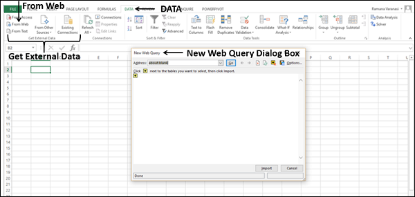
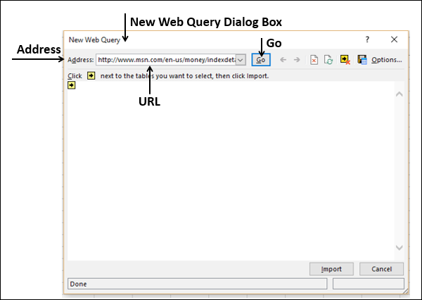
Step 4 − Enter the URL of the web site from where you want to import data, in the box next to Address and click Go.
Step 5 − The data on the website appears. There will be yellow arrow icons next to the table data that can be imported.
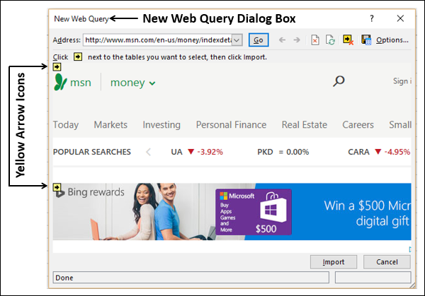
Step 6 − Click the yellow icons to select the data you want to import. This turns the yellow icons to green boxes with a checkmark as shown in the following screen shot.
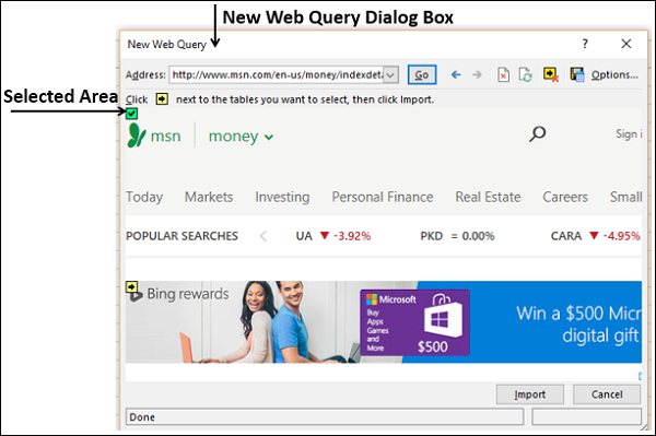
Step 7 − Click the Import button after you have selected what you want.
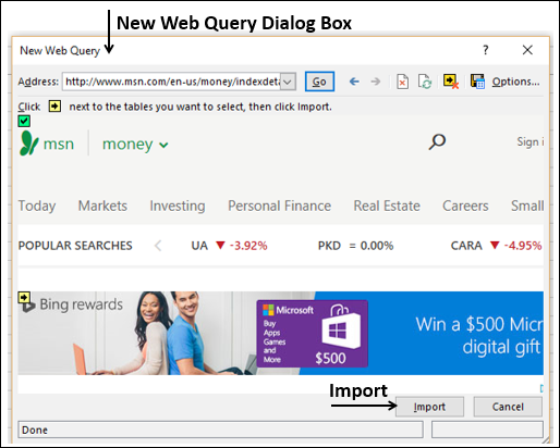
The Import Data dialog box appears.
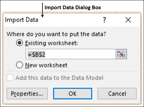
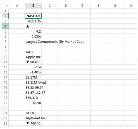
Step 8 − Specify where you want to put the data and click Ok.
Step 9 − Arrange the data for further analysis and/or presentation.
Copy-pasting data from web
Another way of getting data from a web page is by copying and pasting the required data.
Step 1 − Insert a new worksheet.
Step 2 − Copy the data from the web page and paste it on the worksheet.
Step 3 − Create a table with the pasted data.
Importing Data from a Text File
If you have data in .txt or .csv or .prn files, you can import data from those files treating them as text files. Follow the steps given below −
Step 1 − Open a new worksheet in Excel.
Step 2 − Click the DATA tab on the Ribbon.
Step 3 − Click From Text in the Get External Data group. The Import Text File dialog box appears.
You can see that .prn, .txt and .csv extension text files are accepted.
Step 4 − Select the file. The selected file name appears in the File name box. The Open button changes to Import button.
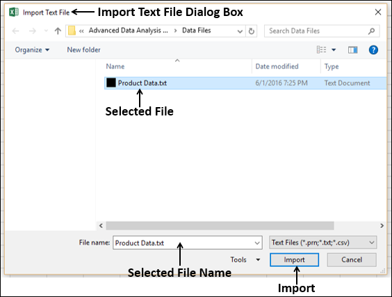
Step 5 − Click the Import button. Text Import Wizard – Step 1 of 3 dialog box appears.
Step 6 − Click the option Delimited to choose the file type and click Next.
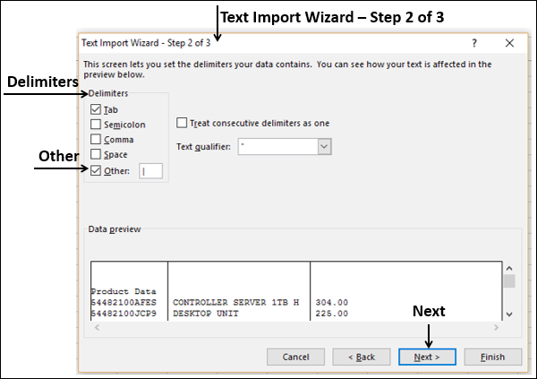
The Text Import Wizard – Step 2 of 3 dialog box appears.
Step 7 − Under Delimiters, select Other.
Step 8 − In the box next to Other, type | (That is the delimiter in the text file you are importing).
Step 9 − Click Next.
The Text Import Wizard – Step 3 of 3 dialog box appears.
Step 10 − In this dialog box, you can set column data format for each of the columns.
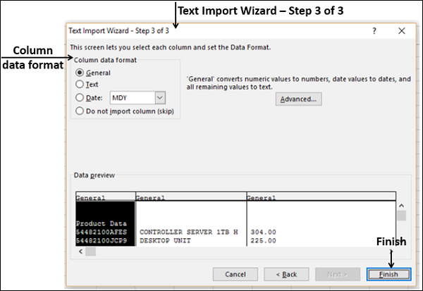
Step 11 − After you complete the data formatting of columns, click Finish. The Import Data dialog box appears.
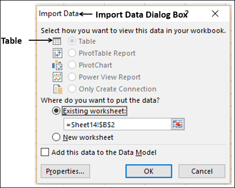
You will observe the following −
-
Table is selected for view and is grayed. Table is the only view option you have in this case.
-
You can put the data either in an existing worksheet or a New worksheet.
-
You can select or not select the check box Add this data to the Data Model.
-
Click OK after you have made the choices.
Data appears on the worksheet you specified. You have imported data from Text file into Excel workbook.
Importing Data from another Workbook
You might have to use data from another Excel workbook for your data analysis, but someone else might maintain the other workbook.
To get up to date data from another workbook, establish a data connection with that workbook.
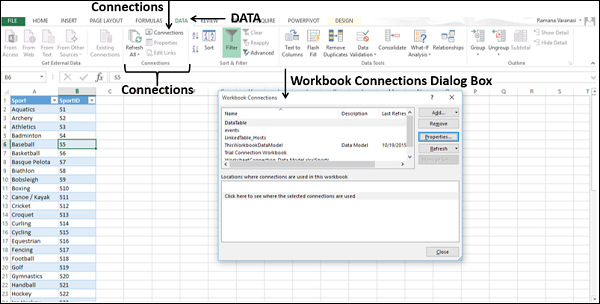
Step 1 − Click DATA > Connections in the Connections group on the Ribbon.
The Workbook Connections dialog box appears.
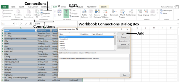
Step 2 − Click the Add button in the Workbook Connections dialog box. The Existing Connections dialog box appears.
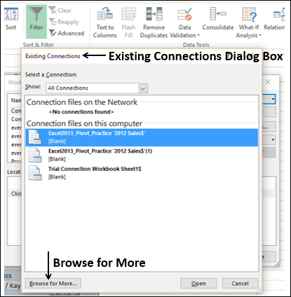
Step 3 − Click Browse for More… button. The Select Data Source dialog box appears.
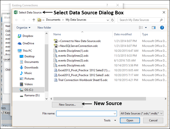
Step 4 − Click the New Source button. The Data Connection Wizard dialog box appears.
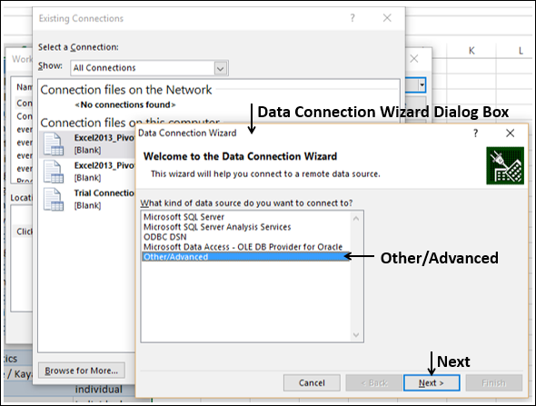
Step 5 − Select Other/Advanced in the data source list and click Next. The Data Link Properties dialog box appears.
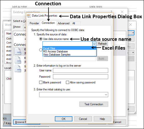
Step 6 − Set the data link properties as follows −
-
Click the Connection tab.
-
Click Use data source name.
-
Click the down-arrow and select Excel Files from the drop-down list.
-
Click OK.
The Select Workbook dialog box appears.
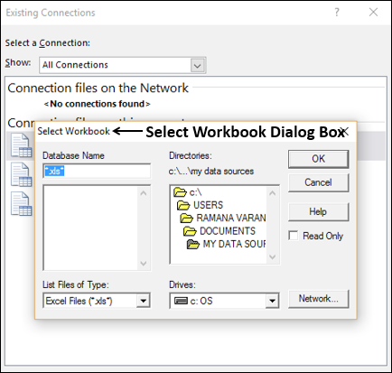
Step 7 − Browse to the location where you have the workbook to be imported is located. Click OK.
The Data Connection Wizard dialog box appears with Select Database and Table.
Note − In this case, Excel treats each worksheet that is getting imported as a table. The table name will be the worksheet name. So, to have meaningful table names, name / rename the worksheets as appropriate.
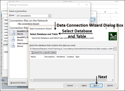
Step 8 − Click Next. The Data Connection Wizard dialog box appears with Save Data Connection File and Finish.
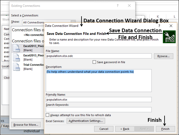
Step 9 − Click the Finish button. The Select Table dialog box appears.
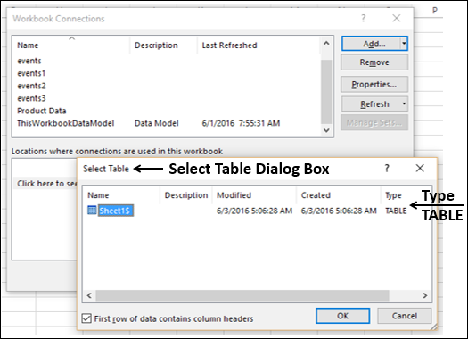
As you observe, Name is the worksheet name that is imported as type TABLE. Click OK.
The Data connection with the workbook you have chosen will be established.
Importing Data from Other Sources
Excel provides you options to choose various other data sources. You can import data from these in few steps.
Step 1 − Open a new blank workbook in Excel.
Step 2 − Click the DATA tab on the Ribbon.
Step 3 − Click From Other Sources in the Get External Data group.
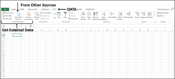
Dropdown with various data sources appears.
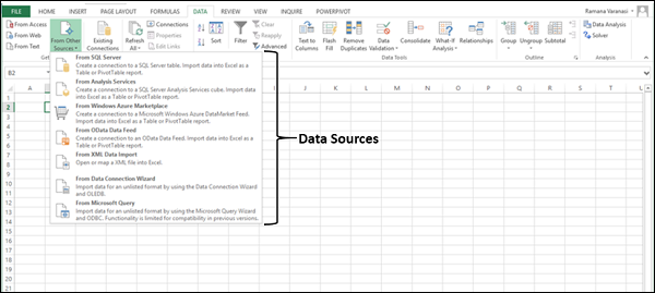
You can import data from any of these data sources into Excel.
Importing Data using an Existing Connection
In an earlier section, you have established a data connection with a workbook.
Now, you can import data using that existing connection.
Step 1 − Click the DATA tab on the Ribbon.
Step 2 − Click Existing Connections in the Get External Data group. The Existing Connections dialog box appears.
Step 3 − Select the connection from where you want to import data and click Open.
Renaming the Data Connections
It will be useful if the data connections you have in your workbook have meaningful names for the ease of understanding and locating.
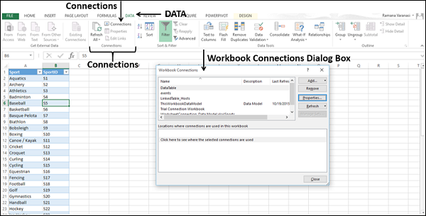
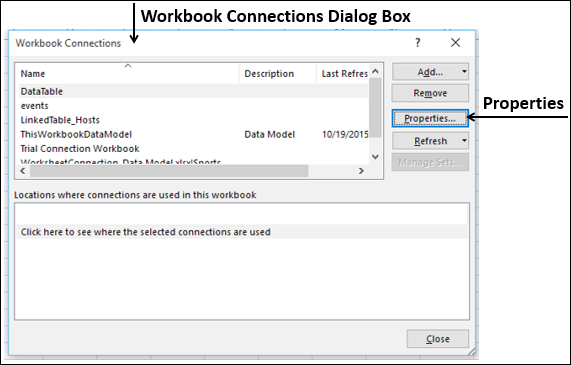
Step 1 − Go to DATA > Connections on the Ribbon. The Workbook Connections dialog box appears.
Step 2 − Select the connection that you want to rename and click Properties.
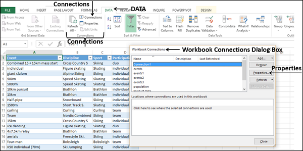
The Connection Properties dialog box appears. The present name appears in the Connection name box −
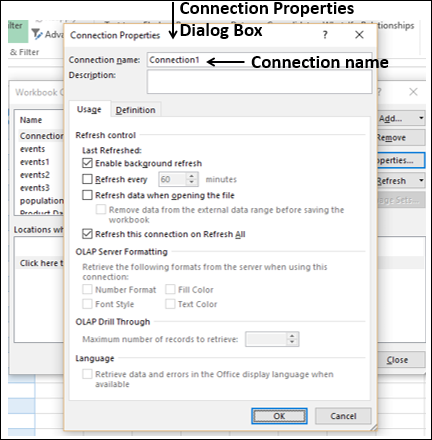
Step 3 − Edit the Connection name and click OK. The data connection will have the new name that you have given.
Refreshing an External Data Connection
When you connect your Excel workbook to an external data source, as you have seen in the above sections, you would like to keep the data in your workbook up to date reflecting the changes made to the external data source time to time.
You can do this by refreshing the data connections you have made to those data sources. Whenever you refresh the data connection, you see the most recent data changes from that data source, including anything that is new or that is modified or that has been deleted.
You can either refresh only the selected data or all the data connections in the workbook at once.
Step 1 − Click the DATA tab on the Ribbon.
Step 2 − Click Refresh All in the Connections group.
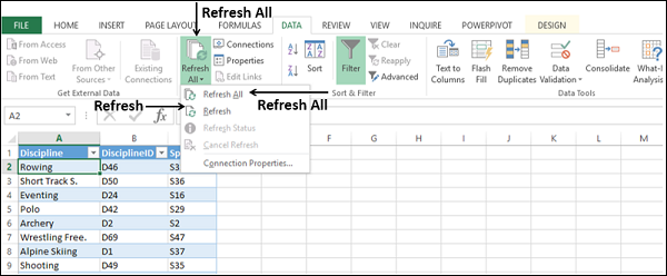
As you observe, there are two commands in the dropdown list – Refresh and Refresh All.
-
If you click Refresh, the selected data in your workbook is updated.
-
If you click Refresh All, all the data connections to your workbook are updated.
Updating all the Data Connections in the Workbook
You might have several data connections to your workbook. You need to update them from time to time so that your workbook will have access to the most recent data.
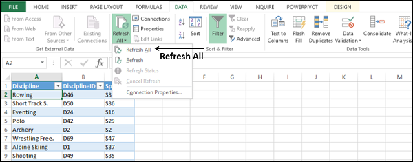
Step 1 − Click any cell in the table that contains the link to the imported data file.
Step 2 − Click the Data tab on the Ribbon.
Step 3 − Click Refresh All in the Connections group.
Step 4 − Select Refresh All from the dropdown list. All the data connections in the workbook will be updated.
Automatically Refresh Data when a Workbook is opened
You might want to have access to the recent data from the data connections to your workbook whenever your workbook is opened.
Step 1 − Click any cell in the table that contains the link to the imported data file.
Step 2 − Click the Data tab.
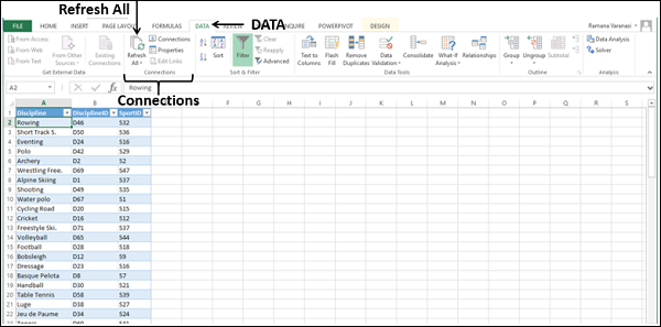
Step 3 − Click Connections in the Connections group.
The Workbook Connections dialog box appears.
Step 4 − Click the Properties button. The Connection Properties dialog box appears.

Step 5 − Click the Usage tab.
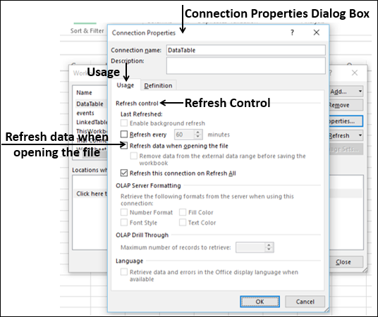
Step 6 − Check the option — Refresh data when opening the file.
You have another option also — Remove data from the external data range before saving the workbook. You can use this option to save the workbook with the query definition but without the external data.
Step 7 − Click OK. Whenever you open your workbook, the up to date data will be loaded into your workbook.
Automatically Refresh Data at regular Intervals
You might be using your workbook keeping it open for longer durations. In such a case, you might want to have the data refreshed periodically without any intervention from you.
Step 1 − Click any cell in the table that contains the link to the imported data file.
Step 2 − Click the Data tab on the Ribbon.
Step 3 − Click Connections in the Connections group.
The Workbook Connections dialog box appears.
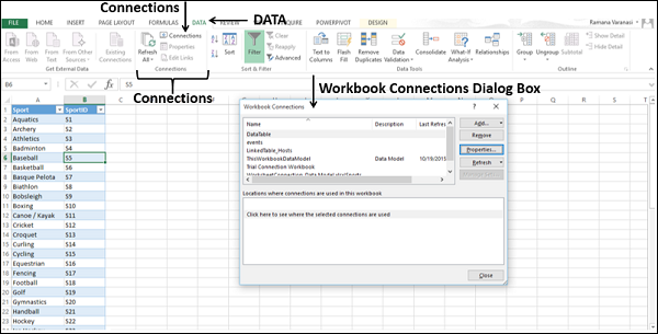
Step 4 − Click the Properties button.

The Connection Properties dialog box appears. Set the properties as follows −
-
Click the Usage tab.
-
Check the option Refresh every.
-
Enter 60 as the number of minutes between each refresh operation and click Ok.
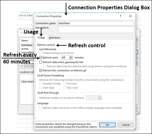
Your Data will be automatically refreshed every 60 min. (i.e. every one hour).
Enabling Background Refresh
For very large data sets, consider running a background refresh. This returns control of Excel to you instead of making you wait several minutes or more for the refresh to finish. You can use this option when you are running a query in the background. However, during this time, you cannot run a query for any connection type that retrieves data for the Data Model.
-
Click in any cell in the table that contains the link to the imported data file.
-
Click the Data tab.
-
Click Connections in the Connections group. The Workbook Connections dialog box appears.
Click the Properties button.
The Connection Properties dialog box appears. Click the Usage tab. The Refresh Control options appear.
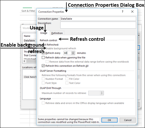
- Click Enable background refresh.
- Click OK. The Background refresh is enabled for your workbook.
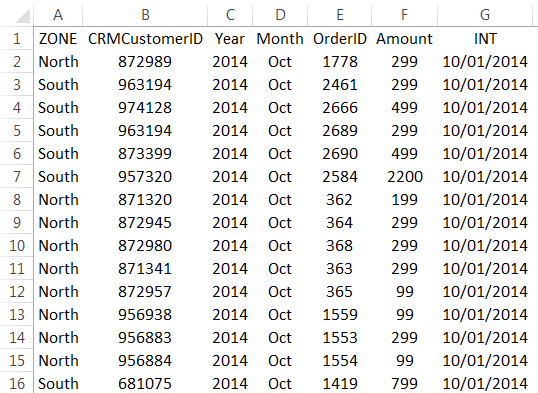
Во-первых, вы можете выбрать свой разделитель. Данные, которые я импортирую, используют запятые для разделения ячеек, поэтому я оставлю запятую выбранной. Вкладка также выбрана, и не оказывает негативного влияния на этот импорт, поэтому я оставлю ее в покое. Если ваша таблица использует пробелы или точки с запятой для различения ячеек, просто выберите этот параметр. Если вы хотите разделить данные на другой символ, такой как косая черта или точка, вы можете ввести этот символ в поле Other : .
Обращайтесь к последовательным разделителям как к одному блоку, делая именно то, что он говорит; в случае запятых наличие двух запятых подряд создаст одну новую ячейку. Если флажок не установлен (по умолчанию), это создаст две новые ячейки.
Текстовое поле имеет важное значение; когда мастер импортирует электронную таблицу, некоторые ячейки будут обрабатываться как числа, а некоторые — как текст. Символ в этом поле сообщит Excel, какие ячейки следует рассматривать как текст. Обычно вокруг текста будут кавычки («»), так что это опция по умолчанию. Текстовые квалификаторы не будут отображаться в окончательной электронной таблице. Вы также можете изменить его на одинарные кавычки (») или ни одного, и в этом случае все кавычки останутся на месте, когда они будут импортированы в окончательную электронную таблицу.
Когда все выглядит хорошо, нажмите Далее>, чтобы перейти к последнему шагу, который позволяет вам установить форматы данных для импортированных ячеек:

Значением по умолчанию для формата данных столбца является « Общее» , которое автоматически преобразует данные в числовой формат, формат даты и текст. По большей части, это будет работать просто отлично. Если у вас есть особые потребности в форматировании, вы можете выбрать Текст или Дата:. Параметр даты также позволяет выбрать формат, в который импортируется дата. И если вы хотите пропустить определенные столбцы, вы можете сделать это тоже.
Каждый из этих параметров применяется к одному или нескольким столбцам, если вы нажмете Shift, чтобы выбрать более одного. Если у вас огромная электронная таблица, таким образом можно пройти через все столбцы таким образом, но это может сэкономить ваше время в долгосрочной перспективе, если все ваши данные будут правильно отформатированы при первом импорте.
Последний параметр в этом диалоговом окне — это меню « Дополнительно» , в котором можно настроить параметры, используемые для распознавания числовых данных. По умолчанию используется точка в качестве десятичного разделителя и запятая в качестве разделителя тысяч, но вы можете изменить это, если ваши данные отформатированы по-разному.

После того, как эти настройки набраны по вашему вкусу, просто нажмите « Готово» и импорт завершен.
Использовать фиксированную ширину вместо разделителей
Если Excel неправильно использует разделители данных или вы импортируете текстовый файл без разделителей , вы можете выбрать фиксированную ширину вместо с разделителями на первом шаге. Это позволяет вам разделить ваши данные на столбцы в зависимости от количества символов в каждом столбце.
Например, если у вас есть электронная таблица, полная ячеек, которая содержит коды с четырьмя буквами и четырьмя цифрами, и вы хотите разделить буквы и цифры между разными ячейками, вы можете выбрать Фиксированная ширина и установить разделение после четырех символов:

Для этого выберите Фиксированная ширина и нажмите Далее> . В следующем диалоговом окне вы можете указать Excel, где разделить данные на разные ячейки, щелкнув отображаемые данные. Чтобы переместить разделение, просто нажмите и перетащите стрелку вверху линии. Если вы хотите удалить разделение, дважды щелкните строку.
После выбора разбиений и нажатия кнопки « Далее>» вы получите те же параметры, что и при импорте с разделителями; Вы можете выбрать формат данных для каждого столбца. Затем нажмите « Готово», и вы получите свою таблицу.

Помимо импорта файлов без разделителей, это хороший способ разделения текста и чисел. из файлов, с которыми вы работаете. Просто сохраните файл как CSV или текстовый файл, импортируйте этот файл и используйте этот метод, чтобы разделить его так, как вы хотите.
Импорт HTML аналогичен импорту CSV или текстовых файлов; выберите файл, выполните те же действия, что и выше, и ваш HTML-документ будет преобразован в электронную таблицу, с которой вы можете работать (это может оказаться полезным, если вы хотите загрузить HTML-таблицы с веб-сайта или если данные веб-формы сохранено в формате HTML).
Экспорт данных из Excel
Экспортировать данные намного проще, чем импортировать их. Когда вы будете готовы к экспорту, нажмите Файл> Сохранить как… (или воспользуйтесь удобным сочетанием клавиш Excel сочетания клавиш ), и вам будет предложен ряд вариантов. Просто выберите тот, который вам нужен.

Вот разбивка нескольких наиболее распространенных:
- .xlsx / .xls : стандартные форматы Excel.
- .xlt : шаблон Excel.
- .xlsb : формат Excel, написанный в двоичном формате вместо XML, который позволяет сохранять очень большие таблицы быстрее, чем стандартные форматы.
- .csv : значение, разделенное запятыми (как в первом примере импорта, использованном выше; может быть прочитано любой программой для работы с электронными таблицами).
- .txt : несколько слегка отличающихся форматов, которые используют вкладки для разделения ячеек в вашей электронной таблице (если есть сомнения, выберите текст с разделителями табуляции вместо другой опции .txt).
Когда вы выбираете формат и нажимаете « Сохранить» , вы можете получить предупреждение, которое выглядит так:

Если вы хотите сохранить файл в формате, отличном от .xlsx или .xls, это может произойти. Если в вашей электронной таблице нет особых функций, которые вам действительно нужны, просто нажмите « Продолжить», и ваш документ будет сохранен.
Один шаг ближе к мастерству в Excel
По большей части люди просто используют таблицы в формате Excel, и их действительно легко открывать, изменять и сохранять. Но время от времени вы будете получать разные документы, например, извлеченные из Интернета или созданные в другом пакете пакет Знание того, как импортировать и экспортировать различные форматы, может сделать работу с такими листами намного удобнее.
Вы импортируете или экспортируете файлы Excel на регулярной основе? Для чего вы считаете это полезным? Есть ли у вас какие-либо советы, чтобы поделиться или конкретные проблемы, для которых вы еще не нашли решение? Поделитесь ими ниже!