
Содержание
- 3 Effective Methods to Get the Path of the Current Excel Workbook
- Method 1: Check Workbook Information
- Method 2: Use Excel Functions
- Method 3: Use VBA Macros
- A Comparison between Those Methods
- Avoid Data Disaster is Next to Impossible
- Insert the current Excel file name, path, or worksheet in a cell
- Insert the current file name, its full path, and the name of the active worksheet
- Insert the current file name and the name of the active worksheet
- Insert the current file name only
- Need more help?
- Extract Filenames from Filepath in Excel
- Method 1: Fetch Filenames Using an Excel Formula
- Method 2: Using a Macro to Get Filename from a Filepath
- Method 3: By using Excel’s Find and Replace Functionality:
- Subscribe and be a part of our 15,000+ member family!
- Insert File Path in Excel
- Get Path and File Name
- File Name, Path, and Worksheet
- FIND the File Name Position
- Remove the Worksheet Name
- SUBSTITUTE Function
- Get Path Only
- Extract the path from a full file-name in VBA
- 5 Answers 5
3 Effective Methods to Get the Path of the Current Excel Workbook
When you are working on an Excel workbook, you may need to refer to the path of this file. In this article, we will show you 3 methods to get the path.
Getting the path of the current workbook seems to be very easy. However, if you close the folder and couldn’t remember the exact location, you will find it hard to get the path especially, especially when there are many files in your computer. You can certainly use the search feature in your computer.
But if there are many files in your computer, you need to spend a lot of time on the search process. On the other hand, if there are many Excel files with the same name in different paths, you will still need to select them one by one. In order to get the path quickly, you can refer to the 3 methods below.
Method 1: Check Workbook Information
This method is very easy. Just click the tab “File” in the ribbon and you can get the information.
Here you will know the complete path of the current workbook. And then you can get access to the path easily.
Method 2: Use Excel Functions
You can only know the exact location of the path of current workbook. If you need to use the path in a worksheet, you can use Excel functions.
- Click the target cell in the worksheet.
- Now input the following formula into this cell”
- And then press the button “Enter” on the keyboard.

After that, you will see the path in the cell. Except for the path and the name of the current file, you can also know the active sheet.
On the other hand, when you don’t need the sheet name, you can also change the formula.
This formula will get the path to the name of the workbook.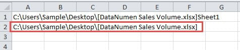
In addition, you can also get only the exact path without the name of the workbook. And the formula will be this:
When you press “Enter” on the keyboard, you will see the result immediately.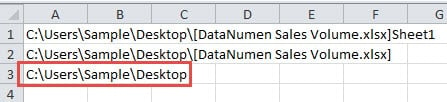
You can choose one of the formulas according to your actual need. When you need to use the path, you can copy it and paste as values. Therefore, only the path will leave in the target cell.
Method 3: Use VBA Macros
Except for the above two methods, you can also use VBA macros to finish this task.
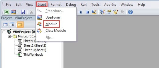
- Press the shortcut keys “Alt +F11” on the keyboard to open the Visual Basic editor.
- And then click the tab “Insert” in the toolbar.
- After that, choose the option “Module” in the sub menu.
- In this step, inputting the following codes into the new module:
There are three different macros in the codes. And for different purpose, the codes will be a little different. The first one will only get the path. The second one will get the path with the file name. And the last one will also get the worksheet name. You may also change the target cell in the codes according to your need.
- When you need to get the path, you can run the macro by clicking the button “Run Sub” or press the button “F5” on the keyboard. Thus, the result will appear in the designated cell.

A Comparison between Those Methods
In this table below, we have input the result of the comparison of the three methods.
Check Workbook Information Use Excel Functions This method will now change the current workbook. You can get 3 different types of the path by the different formulas. With just one click, you can get the result in your worksheet.
If you need to use the path in a cell, you need to spending time inputting the path manually. When you need to use the path itself instead of the result of formulas, you need to paste values only. If you have no idea about VBA, this method will is not suitable for you.
Now you must have a comprehensive understanding of the three methods. And the next time, you can choose the most suitable methods according to your need.
Avoid Data Disaster is Next to Impossible
If you need to use Excel to finish your work, you will certainly deal with a lot of data and information. Therefore, you will sometimes meet with data disaster. And it is impossible that anyone can fully avoid the occurrence of data disaster. When Excel corruption happens, the only thing you can do is to repair it immediately. And in order to repair Excel xlsx file, you can use a third-party tool. This tool is capable of repairing most of the problems in Excel. Therefore, even though you cannot avoid data disaster, you will never lose your data.
Источник
Insert the current Excel file name, path, or worksheet in a cell
Let’s say you want to add information to a spreadsheet report that confirms the location of a workbook and worksheet so you can quickly track and identify it. There are several ways you can do this task.
Insert the current file name, its full path, and the name of the active worksheet
Type or paste the following formula in the cell in which you want to display the current file name with its full path and the name of the current worksheet:
Insert the current file name and the name of the active worksheet
Type or paste the following formula as an array formula to display the current file name and active worksheet name:
=RIGHT(CELL(«filename»),LEN(CELL(«filename»))- MAX(IF(NOT(ISERR(SEARCH(«»,CELL(«filename»), ROW(1:255)))),SEARCH(«»,CELL(«filename»),ROW(1:255)))))
To enter a formula as an array formula, press CTRL+SHIFT+ENTER.
The formula returns the name of the worksheet as long as the worksheet has been saved at least once. If you use this formula on an unsaved worksheet, the formula cell will remain blank until you save the worksheet.
Insert the current file name only
Type or paste the following formula to insert the name of the current file in a cell:
Note: If you use this formula in an unsaved worksheet, you will see the error #VALUE! in the cell. When you save the worksheet, the error is replaced by the file name.
Need more help?
You can always ask an expert in the Excel Tech Community or get support in the Answers community.
Источник
Getting filenames from a Filepath looks like an easy task at first sight. But actually, this is a very cumbersome task when you are dealing with a large number of file paths. Very recently I also wanted to do this task and during the process of extracting filenames, I found few methods that can automate this process.
And today I will be sharing a few methods that can help you to extract filenames from a given list of paths.

The above picture can give you a clear idea of what I am actually talking about.
Method 1: Fetch Filenames Using an Excel Formula
The first and one of the easiest ways to extract the filename from file path is using a formula. The below formula can help you to do the same.

Here in this formula, the only thing that you have to change is the cell position ‘A1’. While using this formula simply replace all the instances of cell position ‘A1’ with the cell position where you have file path present.
How this formula works
I know many of you would be interested to know the logic behind the above formula. I will explain the above formula by breaking it into three parts:
1. First it finds how many “” characters are present in the string. This is accomplished by =LEN(A1)-LEN(SUBSTITUTE(A1,»»,»»)) .
For instance, your file path is “C:SomeFolderFolderFilename.doc” then this part would give you a value “3”.
2. Secondly, it replaces the last “” character of the input string with a “*” character. This is done by =SUBSTITUTE(A1,»»,»*»,LEN(A1)-LEN(SUBSTITUTE(A1,»»,»»)))
For example, if your file path is “C:SomeFolderFolderFilename.doc” then this part of the formula would give you a result “C:SomeFolderFolder*Filename.doc”
3. Now, your job becomes much easier. You only have to extract the part that follows the “*” character. As you maybe already know that this can be easily performed using the MID Function .
Method 2: Using a Macro to Get Filename from a Filepath
If you didn’t like the above formula, then I have created a macro for you. This macro simply replaces the file paths in your predefined range with their corresponding File names. To use this macro follow the below steps:
1. With your excel sheet opened, Press the keys “Alt + F11”.
2. This will open the Excel VBA Editor, after this navigate to Insert > Module.
3. Now paste the below code in the editor.

4. Next, change the cell range (“A1:A10”). You have to change this range with your own range that contains file paths.
5. When you are ready to run the code simply press the “F5” key and all your file paths will be replaced by corresponding filenames.
Method 3: By using Excel’s Find and Replace Functionality:
If you didn’t like either of the two approaches that I have mentioned above then don’t worry here is a much easier alternative for you. This is done by using the Microsoft Excels in-built ‘Find and Replace’ functionality. Follow the below steps to use this functionality to get the filenames from file paths.
1. First of all select the range where you have the FilePaths.
2. Next, press “Ctrl + H”, this will open a ‘Find and Replace’ dialog.

3. In the “Find What” textbox enter “*” (without quotes) and keep the “Replace With” textbox empty. Click “Replace All” and all your Filepaths will be replaced by Filenames.
So, these were some of the methods for getting filenames from file paths. Do drop in your comments if you know any other methods.
Subscribe and be a part of our 15,000+ member family!
Now subscribe to Excel Trick and get a free copy of our ebook «200+ Excel Shortcuts» (printable format) to catapult your productivity.
Источник
Insert File Path in Excel
Download the example workbook
This tutorial will demonstrate how to get the path and file name using a formula in Excel.
Get Path and File Name
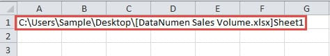
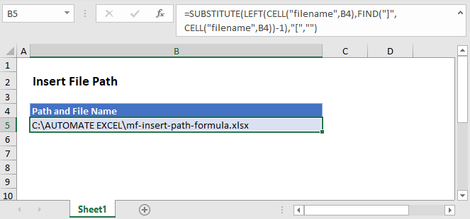
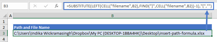
In Excel there isn’t a function to get the path and file name directly, but the CELL Function will return the file path, name, and sheet. Using the text functions FIND, LEFT, and SUBSTITUTE, we can isolate the path and file name.
Let’s step through the formula.
File Name, Path, and Worksheet
We use the CELL Function to return the file path, name, and sheet by entering “filename” as the info type.
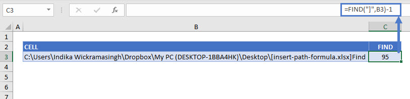
FIND the File Name Position
As shown above, the CELL Function returns the file path, name, and worksheet. We don’t need the worksheet or the square brackets, so we use the FIND function to determine the position of the last character (i.e. the one before “]”) of the file name.
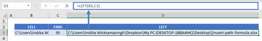
Remove the Worksheet Name
Once we have the position of the file name’s last character, we use the LEFT Function to remove the name of the worksheet.
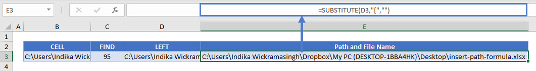
SUBSTITUTE Function
You can see above that there is still an open square bracket between the path and file names. Use the SUBSTITUTE function to replace the “[“ with an empty string.
Combining these steps into a single formula gives us:
Get Path Only
You might want to show the path only, without the file name. For this, we can stop at the LEFT Function with a little tweak. There’s no need to SUBSTITUTE since there won’t be any mid-string characters to delete. To return just the path, we find the position of the first character of the file name (“[“), instead of the last, and the path name is everything to the left.
Источник
I m new in VBA and below is my code which is not working, can any one of u can help?
The above code is not working; my path string is RootzTrash — No longer neededNOCNOC and what I want is RootzTrash — No longer neededNOC.
5 Answers 5
If you want to remove just the last item from your path, you can do it this way:
InStrRev finds the position of the last occurrence of
Left truncates the string until that position
The -1 is because you want also to remove that last
This is useful if you want to remove more than one item (not just the last one) by changing 1 to 2 or 3 for example:

If you are fan of long formulas, this is another option:
- The idea is that you split by
- Then you get the last value in the array (with ubound, but you split twice)
- Then you get the difference between it and the whole length
- Then you pass this difference to the left as a parameter

Approach using Filter() and one Split() action
In addition to @Vityata ‘s answer I demonstrate an array alternative accepting also vbNullString as FullPath argument.
Based on the same idea to make disappear the last split token, this approach doesn’t calculate item lengths, but removes the last item directly via Filter(a, a(Ubound(a)), False) .
Источник
Return to Excel Formulas List
Download Example Workbook
Download the example workbook
This tutorial will demonstrate how to get the path and file name using a formula in Excel.
Get Path and File Name
In Excel there isn’t a function to get the path and file name directly, but the CELL Function will return the file path, name, and sheet. Using the text functions FIND, LEFT, and SUBSTITUTE, we can isolate the path and file name.
=SUBSTITUTE(LEFT(CELL("filename",B2),FIND("]",CELL("filename",B2))-1),"[","")
Let’s step through the formula.
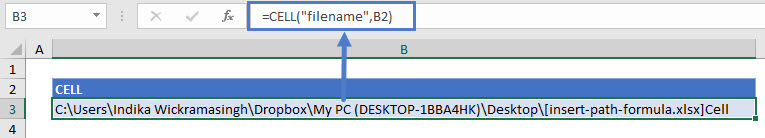
File Name, Path, and Worksheet
We use the CELL Function to return the file path, name, and sheet by entering “filename” as the info type.
=CELL(“filename”,B2)
FIND the File Name Position
As shown above, the CELL Function returns the file path, name, and worksheet. We don’t need the worksheet or the square brackets, so we use the FIND function to determine the position of the last character (i.e. the one before “]”) of the file name.
=FIND("]",B3)-1
Remove the Worksheet Name
Once we have the position of the file name’s last character, we use the LEFT Function to remove the name of the worksheet.
=LEFT(B3,C3)
SUBSTITUTE Function
You can see above that there is still an open square bracket between the path and file names. Use the SUBSTITUTE function to replace the “[“ with an empty string.
=SUBSTITUTE(D3,"[","")
Combining these steps into a single formula gives us:
=SUBSTITUTE(LEFT(CELL("filename",B2),FIND("]",CELL("filename",B2))-1),"[","")Get Path Only
You might want to show the path only, without the file name. For this, we can stop at the LEFT Function with a little tweak. There’s no need to SUBSTITUTE since there won’t be any mid-string characters to delete. To return just the path, we find the position of the first character of the file name (“[“), instead of the last, and the path name is everything to the left.
=LEFT(CELL("filename",B2),FIND("[",CELL("filename",B2))-1)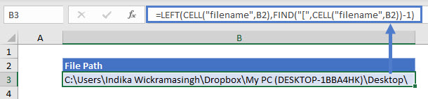
When you are working on an Excel workbook, you may need to refer to the path of this file. In this article, we will show you 3 methods to get the path.
Getting the path of the current workbook seems to be very easy. However, if you close the folder and couldn’t remember the exact location, you will find it hard to get the path especially, especially when there are many files in your computer. You can certainly use the search feature in your computer.
But if there are many files in your computer, you need to spend a lot of time on the search process. On the other hand, if there are many Excel files with the same name in different paths, you will still need to select them one by one. In order to get the path quickly, you can refer to the 3 methods below.
Method 1: Check Workbook Information
This method is very easy. Just click the tab “File” in the ribbon and you can get the information.
Here you will know the complete path of the current workbook. And then you can get access to the path easily.
Method 2: Use Excel Functions
You can only know the exact location of the path of current workbook. If you need to use the path in a worksheet, you can use Excel functions.
- Click the target cell in the worksheet.
- Now input the following formula into this cell”
=CELL(“filename”)
- And then press the button “Enter” on the keyboard.

After that, you will see the path in the cell. Except for the path and the name of the current file, you can also know the active sheet.
On the other hand, when you don’t need the sheet name, you can also change the formula.
= LEFT(CELL(“filename”),FIND(“]”,CELL(“filename”)))
This formula will get the path to the name of the workbook.
In addition, you can also get only the exact path without the name of the workbook. And the formula will be this:
=LEFT(CELL(“filename”),FIND(“[“,CELL(“filename”))-2)
When you press “Enter” on the keyboard, you will see the result immediately.
You can choose one of the formulas according to your actual need. When you need to use the path, you can copy it and paste as values. Therefore, only the path will leave in the target cell.
Method 3: Use VBA Macros
Except for the above two methods, you can also use VBA macros to finish this task.
- Press the shortcut keys “Alt +F11” on the keyboard to open the Visual Basic editor.
- And then click the tab “Insert” in the toolbar.
- After that, choose the option “Module” in the sub menu.

- In this step, inputting the following codes into the new module:
'get only the path
Sub GetPath1()
  Range("B1") = ActiveWorkbook.Path
End Sub

'get the path with the file name
Sub GetPath2()
  Range("B2") = ActiveWorkbook.FullName
End Sub

'get the path with the file name and the sheet name
Sub GetPath3()
  Range("B3") = ActiveWorkbook.FullName & "," & ActiveSheet.Name
End Sub
There are three different macros in the codes. And for different purpose, the codes will be a little different. The first one will only get the path. The second one will get the path with the file name. And the last one will also get the worksheet name. You may also change the target cell in the codes according to your need.
- When you need to get the path, you can run the macro by clicking the button “Run Sub” or press the button “F5” on the keyboard. Thus, the result will appear in the designated cell.
A Comparison between Those Methods
In this table below, we have input the result of the comparison of the three methods.
|
Comparison |
Check Workbook Information | Use Excel Functions |
Use VBA Macros |
|
Advantages |
This method will now change the current workbook. | You can get 3 different types of the path by the different formulas. | With just one click, you can get the result in your worksheet. |
|
Disadvantages |
If you need to use the path in a cell, you need to spending time inputting the path manually. | When you need to use the path itself instead of the result of formulas, you need to paste values only. | If you have no idea about VBA, this method will is not suitable for you. |
Now you must have a comprehensive understanding of the three methods. And the next time, you can choose the most suitable methods according to your need.
Avoid Data Disaster is Next to Impossible
If you need to use Excel to finish your work, you will certainly deal with a lot of data and information. Therefore, you will sometimes meet with data disaster. And it is impossible that anyone can fully avoid the occurrence of data disaster. When Excel corruption happens, the only thing you can do is to repair it immediately. And in order to repair Excel xlsx file, you can use a third-party tool. This tool is capable of repairing most of the problems in Excel. Therefore, even though you cannot avoid data disaster, you will never lose your data.
Author Introduction:
Anna Ma is a data recovery expert in DataNumen, Inc., which is the world leader in data recovery technologies, including repair Word document damage and outlook repair software products. For more information visit www.datanumen.com
Excel for Microsoft 365 Excel 2021 Excel 2019 Excel 2016 Excel 2013 Excel 2010 More…Less
Let’s say you want to add information to a spreadsheet report that confirms the location of a workbook and worksheet so you can quickly track and identify it. There are several ways you can do this task.
Insert the current file name, its full path, and the name of the active worksheet
Type or paste the following formula in the cell in which you want to display the current file name with its full path and the name of the current worksheet:
=CELL(«filename»)
Insert the current file name and the name of the active worksheet
Type or paste the following formula as an array formula to display the current file name and active worksheet name:
=RIGHT(CELL(«filename»),LEN(CELL(«filename»))- MAX(IF(NOT(ISERR(SEARCH(«»,CELL(«filename»), ROW(1:255)))),SEARCH(«»,CELL(«filename»),ROW(1:255)))))
Notes:
-
To enter a formula as an array formula, press CTRL+SHIFT+ENTER.
-
The formula returns the name of the worksheet as long as the worksheet has been saved at least once. If you use this formula on an unsaved worksheet, the formula cell will remain blank until you save the worksheet.
Insert the current file name only
Type or paste the following formula to insert the name of the current file in a cell:
=MID(CELL(«filename»),SEARCH(«[«,CELL(«filename»))+1, SEARCH(«]»,CELL(«filename»))-SEARCH(«[«,CELL(«filename»))-1)
Note: If you use this formula in an unsaved worksheet, you will see the error #VALUE! in the cell. When you save the worksheet, the error is replaced by the file name.
Need more help?
You can always ask an expert in the Excel Tech Community or get support in the Answers community.
Need more help?
Want more options?
Explore subscription benefits, browse training courses, learn how to secure your device, and more.
Communities help you ask and answer questions, give feedback, and hear from experts with rich knowledge.
29 Jun 2014
In several of the template Excel spreadsheets I use in my work there are
references to clients and version numbers that are included. This is for
reference purposes, particularly if the spreadsheet might be printed or
exported as a soft copy (e.g. PDF). Whilst it is possible to maintain
this information manually I decided that this should be something that
could be improved by virtue of the file name containing such information
(as these are the very basis of file management on projects). I’d
referenced the file path and elements of it in the past and I thought
that this would be something that should be relatively straight forward
to achieve; and here’s how I got on ….
The Source
First of all I began by retrieving the file path of the spreadsheet
using the CELL function.
=CELL("filename",A1)
For my rather convoluted example file path (the strange name/path will
be useful later in demonstrating a few things — I’m not suggesting this
would be anything like a real convention!) here’s what it gave.
C:UsersmillasteDesktop[Filename(.xlsx-example) vexed version v1.0.xlsx]Some.Sheet
In my example spreadsheet (available to download below) this is held in
cell B3.
Getting the Folder Path
To get the folder path of the file path, the principle is simply to take
the first character through to (and including) the last back slash. In
order to do this we need to find the character position of the last back
slash so that we can use that with the LEFT function to extract that
number of characters from the full path string.
Unfortunately the FIND function in Excel that is used to locate the
position of a string of text in another string of text has no option to
search a string backwards. Similarly there’s no option to reverse the
character sequence of a string. Whilst this could be achieved with VBA I
prefer to try and accomplish things with standard Excel formulas to
avoid the security implications of relying upon macros. This is a
particularly important consideration when sharing the spreadsheets with
clients.
The workaround is to use the SUBSTITUTE function. SUBSTITUTE allows you
to replace one character string with another character string in the
original string of text. So if we can replace the last back slash with
another character we can then search specifically for that character and
discern the length of the file path. So how does SUBSTITUTE know which
is the last back slash? Well it doesn’t, but you can pass it an optional
parameter to tell it which instance of a character string to replace. So
we simply need to count the number of back slashes and pass that in as a
parameter.
Note a back slash is not a valid file name or Excel worksheet name
character. You may be wondering why I’m not simply searching for the
open square bracket (“[”) instead? Well whilst this isn’t a recommended
file character for use in Excel file names (for what are hopefully
obvious reasons) it is technically possible to include it in the file
name so I went for the back slashes instead.
So how do we count the number of back slashes? Well if we don’t pass the
optional instance parameter to the SUBSTITUTE function it will replace
all instances and our replacement text string could be of zero length
which means if we replace all back slashes with an empty string this
will be the same as deleting them from the string. Comparing the length
of that string (using the LEN function) to the length of the original
string will tell us how many back slashes there are which can then be
passed as an instance to our earlier SUBSTITUTE function.
In cell B6 I output the number of slashes using the following function
combination, the result being 4.
=LEN(B3)-LEN(SUBSTITUTE(B3,"",""))
In cell B7 I output the character position of the last back slash using
the following function combination, the result being 26.
=FIND("*",SUBSTITUTE(B3,"","*",B6),1)
Armed with this position I can then use a simple LEFT function to give
me the folder path (in cell B12).
=LEFT(B3,B7)
The result is C:UsersmillasteDesktop
Getting the File Name
Using a similar principle of locating characters and text replacement we
can also find the file name and extension from the path using the square
brackets as string delimiters. At this point for this example case I’m
assuming that the file name is delimited by the last open square bracket
and the last close square bracket (in case there are any such brackets
in the file path), but I could just as easily have used the length of
the folder path + 1 as the first delimiter.
In the example spreadsheet, cell B8 contains the position of the last
open square bracket; a value of 27.
=FIND("*",SUBSTITUTE(B3,"[","*",LEN(B3)-LEN(SUBSTITUTE(B3,"[",""))),1)
Cell B9 contains the position of the last close square bracket; a value
of 75.
=FIND("*",SUBSTITUTE(B3,"]","*",LEN(B3)-LEN(SUBSTITUTE(B3,"]",""))),1)
Cell B13 then uses the MID function to select the file name based on the
position of the open square bracket and the difference between the
position of the open square bracket and the close square bracket (i.e.
the length of the file name).
=MID(B3,B8+1,B9-B8-1)
The result of this is
Filename(.xlsx-example) vexed version v1.0.xlsx
To remove the file extension we simply use the same sort of combination
of FIND and SUBSTITUTE functions to locate the last period (“.”) in the
file name and take all the text to the left of it. Cell B14 contains the
function to do this.
=LEFT(B13,FIND("*",SUBSTITUTE(B13,".","*",LEN(B13)-LEN(SUBSTITUTE(B13,".",""))),1)-1)
Getting the Worksheet Name
To get the name of the Excel worksheet I simply use the RIGHT formula to
take all of the text in the full file path to the right of the last
close square bracket. The result (Some.Sheet) is shown in cell B15.
=RIGHT(B3,LEN(B3)-B9)
Getting the Version Number
That gives me all of the basic elements from the file path, but I
actually want to extract additional information from the file name. The
example I’m using is a version number. The same principles apply for
working with the text strings, but this time rather than single
character delimiters I’m working with multiple character delimiters.
In the example spreadsheet, the pre-delimiter is “ v” (held in cell B19)
and the post-delimiter is “.xls” (held in cell C19). As long as the
characters appear either side of the desired “attribute” you wish to
extract and are the last instances of
such text in the file name then the combinations I’m sharing here will
work (and are why I’ve chosen such a bizarre file name to illustrate the
example).
The length of the delimiter strings is now important (as they may not
necessarily be a single character — thought they certainly could be) in
carrying out our text string operations.
Cell B20 contains the length of the pre-delimiter (2).
=LEN(B19)
Cell C20 contains the length of the post-delimiter (4).
=LEN(C19)
The next row (21) contains the first set of text substitutions. These
simply replace each of the delimiters with our asterisks.
Cell B21 contains the pre-delimiter substitution
(Filename(.xlsx-example)*exed*ersion*1.0.xlsx).
=SUBSTITUTE(B13,B19,"*")
Cell C21 contains the post-delimiter substitution (Filename(*x-example)
vexed version v1.0*x).
=SUBSTITUTE(B13,C19,"*")
Here’s where the delimiter length comes into play. We need to get the
difference of the lengths between the unsubstituted string and the
substituted string and divide that by the length of the delimiter string
minus one to give us the number of delimiter instances we’re working
with.
Therefore cell B22 contains the number of instances of the pre-delimiter
in the file name (3).
=(LEN(B13)-LEN(SUBSTITUTE(B13,B19,"*")))/(B20-1)
Cell C22 contains the number of instances of the post-delimiter in the
file name (2).
=(LEN(B13)-LEN(SUBSTITUTE(B13,C19,"*")))/(C20-1)
Using this we can then carry out the second set of substitution
operations to replace the last instance of each delimiter.
Cell B23 therefore contains…
=SUBSTITUTE(B13,B19,"*",B22)
Which gives…
Filename(.xlsx-example) vexed version*1.0.xlsx
And cell C23 contains…
=SUBSTITUTE(B13,C19,"*",C22)
Which gives…
Filename(.xlsx-example) vexed version v1.0*x
From this we can now derive the positions of the delimiters using the
FIND function.
Cell B24 contains the position of the last instance of the pre-delimiter
in the file name (38).
=FIND("*",B23)
Cell C24 contains the position of the last instance of the
post-delimiter in the file name (43).
=FIND("*",C23)
Just like getting the file name in the first place, we can then use the
MID function to get the attribute (in this case the version number
remember). The start of the attribute string is the position of the
pre-delimiter plus the length of the pre-delimiter. The length of the
attribute string is the position of the post delimiter minus the sum of
the position of the pre-delimiter and the length of the pre-delimiter.
So cell B26 in the example worksheet contains the version number of 1.0.
=MID(B13,B24+B20,C24-B24-B20)
If you want to get at all of this information you could just create a
worksheet like the Some.Sheet worksheet in the example spreadsheet,
hide it in the workbook and reference the elements as you need them in
other worksheets. If you don’t want to use a hidden worksheet, you could
of course build out the functions rather than build them up over a set
of cells. I’m not advocating this approach as the hidden worksheet is
much easier to maintain and debug, but sometimes it can be handy not to
have hidden worksheets or simply to show off how awesome your Excel
skills are.
The example spreadsheet contains a second worksheet where I’ve done just
that and there are a few examples from that worksheet shown below, but
I’m sure by now you might want a copy of the spreadsheet so here’s the download link.
All In One
Folder Path
=LEFT(CELL("filename",A1),FIND("*",SUBSTITUTE(CELL("filename",A1),"","*",LEN(CELL("filename",A1))-LEN(SUBSTITUTE(CELL("filename",A1),"",""))),1))
File Name (with file extension)
=MID(CELL("filename",A1),FIND("*",SUBSTITUTE(CELL("filename",A1),"[","*",LEN(CELL("filename",A1))-LEN(SUBSTITUTE(CELL("filename",A1),"[",""))),1)+1,FIND("*",SUBSTITUTE(CELL("filename",A1),"]","*",LEN(CELL("filename",A1))-LEN(SUBSTITUTE(CELL("filename",A1),"]",""))),1)-FIND("*",SUBSTITUTE(CELL("filename",A1),"[","*",LEN(CELL("filename",A1))-LEN(SUBSTITUTE(CELL("filename",A1),"[",""))),1)-1)
File Name (without file extension)
=LEFT(MID(CELL("filename",A1),FIND("*",SUBSTITUTE(CELL("filename",A1),"[","*",LEN(CELL("filename",A1))-LEN(SUBSTITUTE(CELL("filename",A1),"[",""))),1)+1,FIND("*",SUBSTITUTE(CELL("filename",A1),"]","*",LEN(CELL("filename",A1))-LEN(SUBSTITUTE(CELL("filename",A1),"]",""))),1)-FIND("*",SUBSTITUTE(CELL("filename",A1),"[","*",LEN(CELL("filename",A1))-LEN(SUBSTITUTE(CELL("filename",A1),"[",""))),1)-1),FIND("*",SUBSTITUTE(MID(CELL("filename",A1),FIND("*",SUBSTITUTE(CELL("filename",A1),"[","*",LEN(CELL("filename",A1))-LEN(SUBSTITUTE(CELL("filename",A1),"[",""))),1)+1,FIND("*",SUBSTITUTE(CELL("filename",A1),"]","*",LEN(CELL("filename",A1))-LEN(SUBSTITUTE(CELL("filename",A1),"]",""))),1)-FIND("*",SUBSTITUTE(CELL("filename",A1),"[","*",LEN(CELL("filename",A1))-LEN(SUBSTITUTE(CELL("filename",A1),"[",""))),1)-1),".","*",LEN(MID(CELL("filename",A1),FIND("*",SUBSTITUTE(CELL("filename",A1),"[","*",LEN(CELL("filename",A1))-LEN(SUBSTITUTE(CELL("filename",A1),"[",""))),1)+1,FIND("*",SUBSTITUTE(CELL("filename",A1),"]","*",LEN(CELL("filename",A1))-LEN(SUBSTITUTE(CELL("filename",A1),"]",""))),1)-FIND("*",SUBSTITUTE(CELL("filename",A1),"[","*",LEN(CELL("filename",A1))-LEN(SUBSTITUTE(CELL("filename",A1),"[",""))),1)-1))-LEN(SUBSTITUTE(MID(CELL("filename",A1),FIND("*",SUBSTITUTE(CELL("filename",A1),"[","*",LEN(CELL("filename",A1))-LEN(SUBSTITUTE(CELL("filename",A1),"[",""))),1)+1,FIND("*",SUBSTITUTE(CELL("filename",A1),"]","*",LEN(CELL("filename",A1))-LEN(SUBSTITUTE(CELL("filename",A1),"]",""))),1)-FIND("*",SUBSTITUTE(CELL("filename",A1),"[","*",LEN(CELL("filename",A1))-LEN(SUBSTITUTE(CELL("filename",A1),"[",""))),1)-1),".",""))),1)-1)
Worksheet Name
=RIGHT(CELL("filename",A1),LEN(CELL("filename",A1))-FIND("*",SUBSTITUTE(CELL("filename",A1),"]","*",LEN(CELL("filename",A1))-LEN(SUBSTITUTE(CELL("filename",A1),"]",""))),1))
Version
=MID(MID(CELL("filename",A1),FIND("*",SUBSTITUTE(CELL("filename",A1),"[","*",LEN(CELL("filename",A1))-LEN(SUBSTITUTE(CELL("filename",A1),"[",""))),1)+1,FIND("*",SUBSTITUTE(CELL("filename",A1),"]","*",LEN(CELL("filename",A1))-LEN(SUBSTITUTE(CELL("filename",A1),"]",""))),1)-FIND("*",SUBSTITUTE(CELL("filename",A1),"[","*",LEN(CELL("filename",A1))-LEN(SUBSTITUTE(CELL("filename",A1),"[",""))),1)-1),FIND("*",SUBSTITUTE(MID(CELL("filename",A1),FIND("*",SUBSTITUTE(CELL("filename",A1),"[","*",LEN(CELL("filename",A1))-LEN(SUBSTITUTE(CELL("filename",A1),"[",""))),1)+1,FIND("*",SUBSTITUTE(CELL("filename",A1),"]","*",LEN(CELL("filename",A1))-LEN(SUBSTITUTE(CELL("filename",A1),"]",""))),1)-FIND("*",SUBSTITUTE(CELL("filename",A1),"[","*",LEN(CELL("filename",A1))-LEN(SUBSTITUTE(CELL("filename",A1),"[",""))),1)-1)," v","*",(LEN(MID(CELL("filename",A1),FIND("*",SUBSTITUTE(CELL("filename",A1),"[","*",LEN(CELL("filename",A1))-LEN(SUBSTITUTE(CELL("filename",A1),"[",""))),1)+1,FIND("*",SUBSTITUTE(CELL("filename",A1),"]","*",LEN(CELL("filename",A1))-LEN(SUBSTITUTE(CELL("filename",A1),"]",""))),1)-FIND("*",SUBSTITUTE(CELL("filename",A1),"[","*",LEN(CELL("filename",A1))-LEN(SUBSTITUTE(CELL("filename",A1),"[",""))),1)-1))-LEN(SUBSTITUTE(MID(CELL("filename",A1),FIND("*",SUBSTITUTE(CELL("filename",A1),"[","*",LEN(CELL("filename",A1))-LEN(SUBSTITUTE(CELL("filename",A1),"[",""))),1)+1,FIND("*",SUBSTITUTE(CELL("filename",A1),"]","*",LEN(CELL("filename",A1))-LEN(SUBSTITUTE(CELL("filename",A1),"]",""))),1)-FIND("*",SUBSTITUTE(CELL("filename",A1),"[","*",LEN(CELL("filename",A1))-LEN(SUBSTITUTE(CELL("filename",A1),"[",""))),1)-1)," v","*")))/(LEN(" v")-1)))+LEN(" v"),FIND("*",SUBSTITUTE(MID(CELL("filename",A1),FIND("*",SUBSTITUTE(CELL("filename",A1),"[","*",LEN(CELL("filename",A1))-LEN(SUBSTITUTE(CELL("filename",A1),"[",""))),1)+1,FIND("*",SUBSTITUTE(CELL("filename",A1),"]","*",LEN(CELL("filename",A1))-LEN(SUBSTITUTE(CELL("filename",A1),"]",""))),1)-FIND("*",SUBSTITUTE(CELL("filename",A1),"[","*",LEN(CELL("filename",A1))-LEN(SUBSTITUTE(CELL("filename",A1),"[",""))),1)-1),".xls","*",(LEN(MID(CELL("filename",A1),FIND("*",SUBSTITUTE(CELL("filename",A1),"[","*",LEN(CELL("filename",A1))-LEN(SUBSTITUTE(CELL("filename",A1),"[",""))),1)+1,FIND("*",SUBSTITUTE(CELL("filename",A1),"]","*",LEN(CELL("filename",A1))-LEN(SUBSTITUTE(CELL("filename",A1),"]",""))),1)-FIND("*",SUBSTITUTE(CELL("filename",A1),"[","*",LEN(CELL("filename",A1))-LEN(SUBSTITUTE(CELL("filename",A1),"[",""))),1)-1))-LEN(SUBSTITUTE(MID(CELL("filename",A1),FIND("*",SUBSTITUTE(CELL("filename",A1),"[","*",LEN(CELL("filename",A1))-LEN(SUBSTITUTE(CELL("filename",A1),"[",""))),1)+1,FIND("*",SUBSTITUTE(CELL("filename",A1),"]","*",LEN(CELL("filename",A1))-LEN(SUBSTITUTE(CELL("filename",A1),"]",""))),1)-FIND("*",SUBSTITUTE(CELL("filename",A1),"[","*",LEN(CELL("filename",A1))-LEN(SUBSTITUTE(CELL("filename",A1),"[",""))),1)-1),".xls","*")))/(LEN(".xls")-1)))-FIND("*",SUBSTITUTE(MID(CELL("filename",A1),FIND("*",SUBSTITUTE(CELL("filename",A1),"[","*",LEN(CELL("filename",A1))-LEN(SUBSTITUTE(CELL("filename",A1),"[",""))),1)+1,FIND("*",SUBSTITUTE(CELL("filename",A1),"]","*",LEN(CELL("filename",A1))-LEN(SUBSTITUTE(CELL("filename",A1),"]",""))),1)-FIND("*",SUBSTITUTE(CELL("filename",A1),"[","*",LEN(CELL("filename",A1))-LEN(SUBSTITUTE(CELL("filename",A1),"[",""))),1)-1)," v","*",(LEN(MID(CELL("filename",A1),FIND("*",SUBSTITUTE(CELL("filename",A1),"[","*",LEN(CELL("filename",A1))-LEN(SUBSTITUTE(CELL("filename",A1),"[",""))),1)+1,FIND("*",SUBSTITUTE(CELL("filename",A1),"]","*",LEN(CELL("filename",A1))-LEN(SUBSTITUTE(CELL("filename",A1),"]",""))),1)-FIND("*",SUBSTITUTE(CELL("filename",A1),"[","*",LEN(CELL("filename",A1))-LEN(SUBSTITUTE(CELL("filename",A1),"[",""))),1)-1))-LEN(SUBSTITUTE(MID(CELL("filename",A1),FIND("*",SUBSTITUTE(CELL("filename",A1),"[","*",LEN(CELL("filename",A1))-LEN(SUBSTITUTE(CELL("filename",A1),"[",""))),1)+1,FIND("*",SUBSTITUTE(CELL("filename",A1),"]","*",LEN(CELL("filename",A1))-LEN(SUBSTITUTE(CELL("filename",A1),"]",""))),1)-FIND("*",SUBSTITUTE(CELL("filename",A1),"[","*",LEN(CELL("filename",A1))-LEN(SUBSTITUTE(CELL("filename",A1),"[",""))),1)-1)," v","*")))/(LEN(" v")-1)))-LEN(" v"))
Summary
The same methods can of course be used to extract other attributes of
the file name or even for example the parent folder (last folder in the
file path) if that were relevant. As long as you can define the
delimiters reliably and they are either the first or the last, you
should be able to get the data you want programmatically.