
Abstract: This is the first tutorial in a series designed to get you acquainted and comfortable using Excel and its built-in data mash-up and analysis features. These tutorials build and refine an Excel workbook from scratch, build a data model, then create amazing interactive reports using Power View. The tutorials are designed to demonstrate Microsoft Business Intelligence features and capabilities in Excel, PivotTables, Power Pivot, and Power View.
Note: This article describes data models in Excel 2013. However, the same data modeling and Power Pivot features introduced in Excel 2013 also apply to Excel 2016.
In these tutorials you learn how to import and explore data in Excel, build and refine a data model using Power Pivot, and create interactive reports with Power View that you can publish, protect, and share.
The tutorials in this series are the following:
-
Import Data into Excel 2013, and Create a Data Model
-
Extend Data Model relationships using Excel, Power Pivot, and DAX
-
Create Map-based Power View Reports
-
Incorporate Internet Data, and Set Power View Report Defaults
-
Power Pivot Help
-
Create Amazing Power View Reports — Part 2
In this tutorial, you start with a blank Excel workbook.
The sections in this tutorial are the following:
-
Import data from a database
-
Import data from a spreadsheet
-
Import data using copy and paste
-
Create a relationship between imported data
-
Checkpoint and Quiz
At the end of this tutorial is a quiz you can take to test your learning.
This tutorial series uses data describing Olympic Medals, hosting countries, and various Olympic sporting events. We suggest you go through each tutorial in order. Also, tutorials use Excel 2013 with Power Pivot enabled. For more information on Excel 2013, click here. For guidance on enabling Power Pivot, click here.
Import data from a database
We start this tutorial with a blank workbook. The goal in this section is to connect to an external data source, and import that data into Excel for further analysis.
Let’s start by downloading some data from the Internet. The data describes Olympic Medals, and is a Microsoft Access database.
-
Click the following links to download files we use during this tutorial series. Download each of the four files to a location that’s easily accessible, such as Downloads or My Documents, or to a new folder you create:
> OlympicMedals.accdb Access database
> OlympicSports.xlsx Excel workbook
> Population.xlsx Excel workbook
> DiscImage_table.xlsx Excel workbook -
In Excel 2013, open a blank workbook.
-
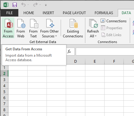
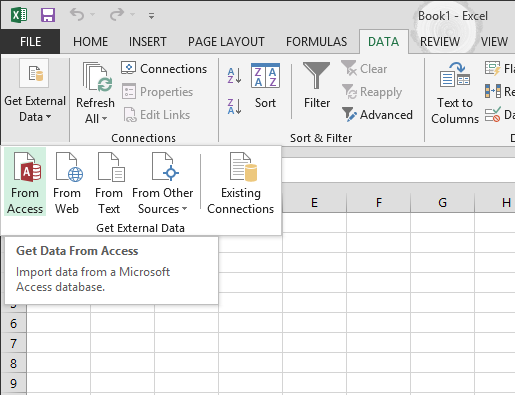
Click DATA > Get External Data > From Access. The ribbon adjusts dynamically based on the width of your workbook, so the commands on your ribbon may look slightly different from the following screens. The first screen shows the ribbon when a workbook is wide, the second image shows a workbook that has been resized to take up only a portion of the screen.

-
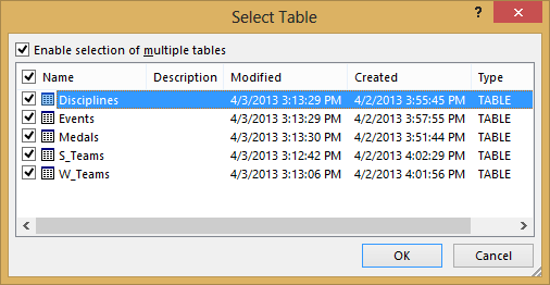
Select the OlympicMedals.accdb file you downloaded and click Open. The following Select Table window appears, displaying the tables found in the database. Tables in a database are similar to worksheets or tables in Excel. Check the Enable selection of multiple tables box, and select all the tables. Then click OK.
-
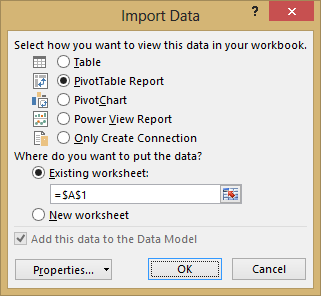
The Import Data window appears.
Note: Notice the checkbox at the bottom of the window that allows you to Add this data to the Data Model, shown in the following screen. A Data Model is created automatically when you import or work with two or more tables simultaneously. A Data Model integrates the tables, enabling extensive analysis using PivotTables, Power Pivot, and Power View. When you import tables from a database, the existing database relationships between those tables is used to create the Data Model in Excel. The Data Model is transparent in Excel, but you can view and modify it directly using the Power Pivot add-in. The Data Model is discussed in more detail later in this tutorial.
Select the PivotTable Report option, which imports the tables into Excel and prepares a PivotTable for analyzing the imported tables, and click OK.
-
Once the data is imported, a PivotTable is created using the imported tables.
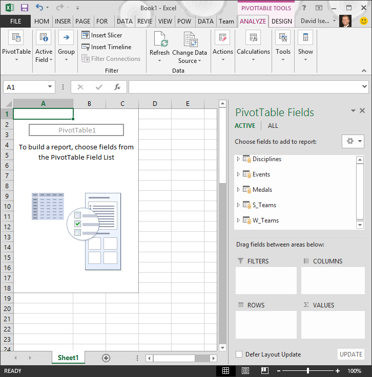
With the data imported into Excel, and the Data Model automatically created, you’re ready to explore the data.
Explore data using a PivotTable
Exploring imported data is easy using a PivotTable. In a PivotTable, you drag fields (similar to columns in Excel) from tables (like the tables you just imported from the Access database) into different areas of the PivotTable to adjust how it presents your data. A PivotTable has four areas: FILTERS, COLUMNS, ROWS, and VALUES.
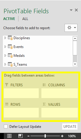
It might take some experimenting to determine which area a field should be dragged to. You can drag as many or few fields from your tables as you like, until the PivotTable presents your data how you want to see it. Feel free to explore by dragging fields into different areas of the PivotTable; the underlying data is not affected when you arrange fields in a PivotTable.
Let’s explore the Olympic Medals data in the PivotTable, starting with Olympic medalists organized by discipline, medal type, and the athlete’s country or region.
-
In PivotTable Fields, expand the Medals table by clicking the arrow beside it. Find the NOC_CountryRegion field in the expanded Medals table, and drag it to the COLUMNS area. NOC stands for National Olympic Committees, which is the organizational unit for a country or region.
-
Next, from the Disciplines table, drag Discipline to the ROWS area.
-
Let’s filter Disciplines to display only five sports: Archery, Diving, Fencing, Figure Skating, and Speed Skating. You can do this from within the PivotTable Fields area, or from the Row Labels filter in the PivotTable itself.
-
Click anywhere in the PivotTable to ensure the Excel PivotTable is selected. In the PivotTable Fields list, where the Disciplines table is expanded, hover over its Discipline field and a dropdown arrow appears to the right of the field. Click the dropdown, click (Select All)to remove all selections, then scroll down and select Archery, Diving, Fencing, Figure Skating, and Speed Skating. Click OK.
-
Or, in the Row Labels section of the PivotTable, click the dropdown next to Row Labels in the PivotTable, click (Select All) to remove all selections, then scroll down and select Archery, Diving, Fencing, Figure Skating, and Speed Skating. Click OK.
-
-
In PivotTable Fields, from the Medals table, drag Medal to the VALUES area. Since Values must be numeric, Excel automatically changes Medal to Count of Medal.
-
From the Medals table, select Medal again and drag it into the FILTERS area.
-
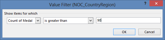
Let’s filter the PivotTable to display only those countries or regions with more than 90 total medals. Here’s how.
-
In the PivotTable, click the dropdown to the right of Column Labels.
-
Select Value Filters and select Greater Than….
-
Type 90 in the last field (on the right). Click OK.
-
Your PivotTable looks like the following screen.
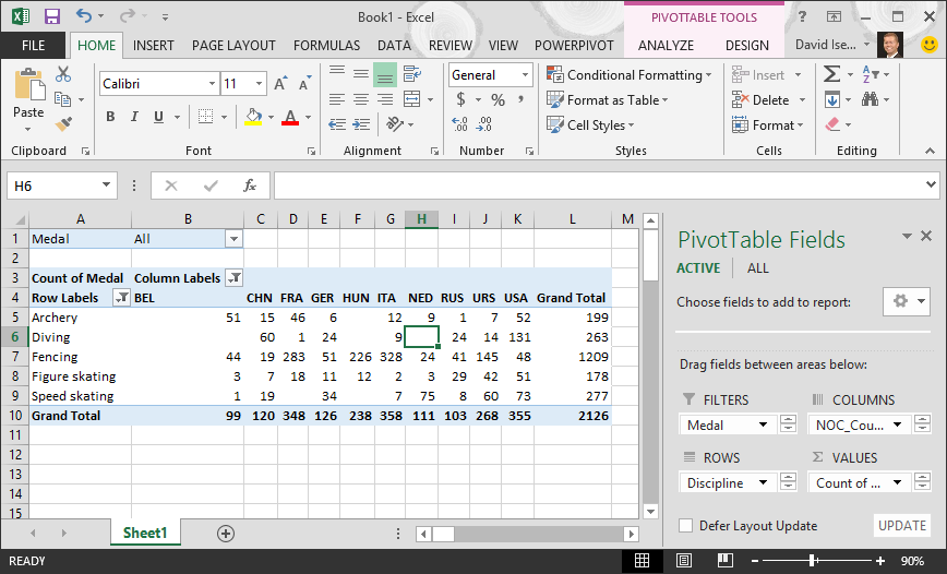
With little effort, you now have a basic PivotTable that includes fields from three different tables. What made this task so simple were the pre-existing relationships among the tables. Because table relationships existed in the source database, and because you imported all the tables in a single operation, Excel could recreate those table relationships in its Data Model.
But what if your data originates from different sources, or is imported at a later time? Typically, you can create relationships with new data based on matching columns. In the next step, you import additional tables, and learn how to create new relationships.
Import data from a spreadsheet
Now let’s import data from another source, this time from an existing workbook, then specify the relationships between our existing data and the new data. Relationships let you analyze collections of data in Excel, and create interesting and immersive visualizations from the data you import.
Let’s start by creating a blank worksheet, then import data from an Excel workbook.
-
Insert a new Excel worksheet, and name it Sports.
-
Browse to the folder that contains the downloaded sample data files, and open OlympicSports.xlsx.
-
Select and copy the data in Sheet1. If you select a cell with data, such as cell A1, you can press Ctrl + A to select all adjacent data. Close the OlympicSports.xlsx workbook.
-
On the Sports worksheet, place your cursor in cell A1 and paste the data.
-
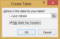
With the data still highlighted, press Ctrl + T to format the data as a table. You can also format the data as a table from the ribbon by selecting HOME > Format as Table. Since the data has headers, select My table has headers in the Create Table window that appears, as shown here.
Formatting the data as a table has many advantages. You can assign a name to a table, which makes it easy to identify. You can also establish relationships between tables, enabling exploration and analysis in PivotTables, Power Pivot, and Power View.
-
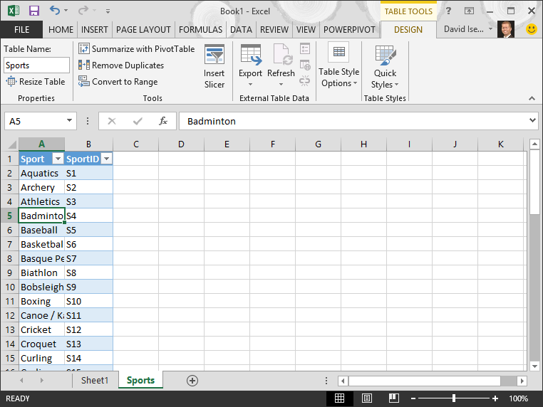
Name the table. In TABLE TOOLS > DESIGN > Properties, locate the Table Name field and type Sports. The workbook looks like the following screen.
-
Save the workbook.
Import data using copy and paste
Now that we’ve imported data from an Excel workbook, let’s import data from a table we find on a web page, or any other source from which we can copy and paste into Excel. In the following steps, you add the Olympic host cities from a table.
-
Insert a new Excel worksheet, and name it Hosts.
-
Select and copy the following table, including the table headers.
|
City |
NOC_CountryRegion |
Alpha-2 Code |
Edition |
Season |
|
Melbourne / Stockholm |
AUS |
AS |
1956 |
Summer |
|
Sydney |
AUS |
AS |
2000 |
Summer |
|
Innsbruck |
AUT |
AT |
1964 |
Winter |
|
Innsbruck |
AUT |
AT |
1976 |
Winter |
|
Antwerp |
BEL |
BE |
1920 |
Summer |
|
Antwerp |
BEL |
BE |
1920 |
Winter |
|
Montreal |
CAN |
CA |
1976 |
Summer |
|
Lake Placid |
CAN |
CA |
1980 |
Winter |
|
Calgary |
CAN |
CA |
1988 |
Winter |
|
St. Moritz |
SUI |
SZ |
1928 |
Winter |
|
St. Moritz |
SUI |
SZ |
1948 |
Winter |
|
Beijing |
CHN |
CH |
2008 |
Summer |
|
Berlin |
GER |
GM |
1936 |
Summer |
|
Garmisch-Partenkirchen |
GER |
GM |
1936 |
Winter |
|
Barcelona |
ESP |
SP |
1992 |
Summer |
|
Helsinki |
FIN |
FI |
1952 |
Summer |
|
Paris |
FRA |
FR |
1900 |
Summer |
|
Paris |
FRA |
FR |
1924 |
Summer |
|
Chamonix |
FRA |
FR |
1924 |
Winter |
|
Grenoble |
FRA |
FR |
1968 |
Winter |
|
Albertville |
FRA |
FR |
1992 |
Winter |
|
London |
GBR |
UK |
1908 |
Summer |
|
London |
GBR |
UK |
1908 |
Winter |
|
London |
GBR |
UK |
1948 |
Summer |
|
Munich |
GER |
DE |
1972 |
Summer |
|
Athens |
GRC |
GR |
2004 |
Summer |
|
Cortina d’Ampezzo |
ITA |
IT |
1956 |
Winter |
|
Rome |
ITA |
IT |
1960 |
Summer |
|
Turin |
ITA |
IT |
2006 |
Winter |
|
Tokyo |
JPN |
JA |
1964 |
Summer |
|
Sapporo |
JPN |
JA |
1972 |
Winter |
|
Nagano |
JPN |
JA |
1998 |
Winter |
|
Seoul |
KOR |
KS |
1988 |
Summer |
|
Mexico |
MEX |
MX |
1968 |
Summer |
|
Amsterdam |
NED |
NL |
1928 |
Summer |
|
Oslo |
NOR |
NO |
1952 |
Winter |
|
Lillehammer |
NOR |
NO |
1994 |
Winter |
|
Stockholm |
SWE |
SW |
1912 |
Summer |
|
St Louis |
USA |
US |
1904 |
Summer |
|
Los Angeles |
USA |
US |
1932 |
Summer |
|
Lake Placid |
USA |
US |
1932 |
Winter |
|
Squaw Valley |
USA |
US |
1960 |
Winter |
|
Moscow |
URS |
RU |
1980 |
Summer |
|
Los Angeles |
USA |
US |
1984 |
Summer |
|
Atlanta |
USA |
US |
1996 |
Summer |
|
Salt Lake City |
USA |
US |
2002 |
Winter |
|
Sarajevo |
YUG |
YU |
1984 |
Winter |
-
In Excel, place your cursor in cell A1 of the Hosts worksheet and paste the data.
-
Format the data as a table. As described earlier in this tutorial, you press Ctrl + T to format the data as a table, or from HOME > Format as Table. Since the data has headers, select My table has headers in the Create Table window that appears.
-
Name the table. In TABLE TOOLS > DESIGN > Properties locate the Table Name field, and type Hosts.
-
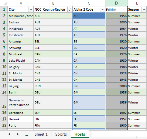
Select the Edition column, and from the HOME tab, format it as Number with 0 decimal places.
-
Save the workbook. Your workbook looks like the following screen.
Now that you have an Excel workbook with tables, you can create relationships between them. Creating relationships between tables lets you mash up the data from the two tables.
Create a relationship between imported data
You can immediately begin using fields in your PivotTable from the imported tables. If Excel can’t determine how to incorporate a field into the PivotTable, a relationship must be established with the existing Data Model. In the following steps, you learn how to create a relationship between data you imported from different sources.
-
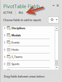
On Sheet1, at the top ofPivotTable Fields, clickAll to view the complete list of available tables, as shown in the following screen.
-
Scroll through the list to see the new tables you just added.
-
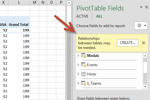
Expand Sports and select Sport to add it to the PivotTable. Notice that Excel prompts you to create a relationship, as seen in the following screen.
This notification occurs because you used fields from a table that’s not part of the underlying Data Model. One way to add a table to the Data Model is to create a relationship to a table that’s already in the Data Model. To create the relationship, one of the tables must have a column of unique, non-repeated, values. In the sample data, the Disciplines table imported from the database contains a field with sports codes, called SportID. Those same sports codes are present as a field in the Excel data we imported. Let’s create the relationship.
-
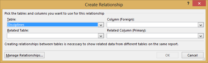
Click CREATE… in the highlighted PivotTable Fields area to open the Create Relationship dialog, as shown in the following screen.
-
In Table, choose Disciplines from the drop down list.
-
In Column (Foreign), choose SportID.
-
In Related Table, choose Sports.
-
In Related Column (Primary), choose SportID.
-
Click OK.
The PivotTable changes to reflect the new relationship. But the PivotTable doesn’t look right quite yet, because of the ordering of fields in the ROWS area. Discipline is a subcategory of a given sport, but since we arranged Discipline above Sport in the ROWS area, it’s not organized properly. The following screen shows this unwanted ordering.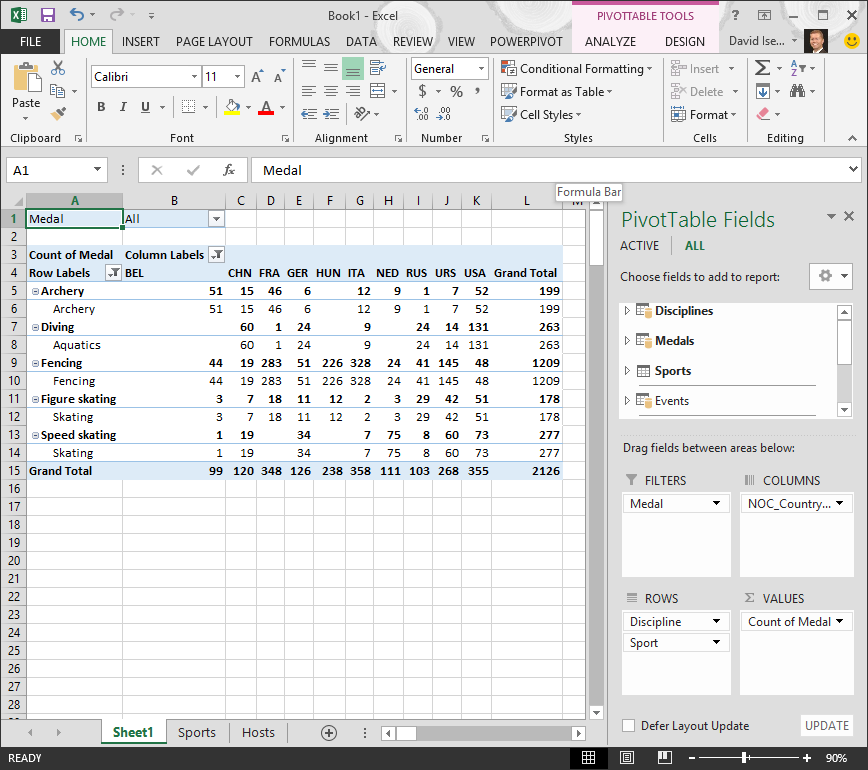
-
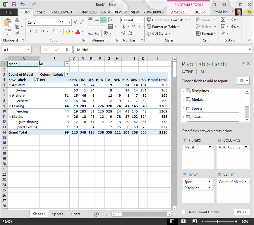
In the ROWS area, move Sport above Discipline. That’s much better, and the PivotTable displays the data how you want to see it, as shown in the following screen.
Behind the scenes, Excel is building a Data Model that can be used throughout the workbook, in any PivotTable, PivotChart, in Power Pivot, or any Power View report. Table relationships are the basis of a Data Model, and what determine navigation and calculation paths.
In the next tutorial, Extend Data Model relationships using Excel 2013, Power Pivot, and DAX, you build on what you learned here, and step through extending the Data Model using a powerful and visual Excel add-in called Power Pivot. You also learn how to calculate columns in a table, and use that calculated column so that an otherwise unrelated table can be added to your Data Model.
Checkpoint and Quiz
Review What You’ve Learned
You now have an Excel workbook that includes a PivotTable accessing data in multiple tables, several of which you imported separately. You learned to import from a database, from another Excel workbook, and from copying data and pasting it into Excel.
To make the data work together, you had to create a table relationship that Excel used to correlate the rows. You also learned that having columns in one table that correlate to data in another table is essential for creating relationships, and for looking up related rows.
You’re ready for the next tutorial in this series. Here’s a link:
Extend Data Model relationships using Excel 2013, Power Pivot, and DAX
QUIZ
Want to see how well you remember what you learned? Here’s your chance. The following quiz highlights features, capabilities, or requirements you learned about in this tutorial. At the bottom of the page, you’ll find the answers. Good luck!
Question 1: Why is it important to convert imported data into tables?
A: You don’t have to convert them into tables, because all imported data is automatically turned into tables.
B: If you convert imported data into tables, they will be excluded from the Data Model. Only when they’re excluded from the Data Model are they available in PivotTables, Power Pivot, and Power View.
C: If you convert imported data into tables, they can be included in the Data Model, and be made available to PivotTables, Power Pivot, and Power View.
D: You cannot convert imported data into tables.
Question 2: Which of the following data sources can you import into Excel, and include in the Data Model?
A: Access Databases, and many other databases as well.
B: Existing Excel files.
C: Anything you can copy and paste into Excel and format as a table, including data tables in websites, documents, or anything else that can be pasted into Excel.
D: All of the above
Question 3: In a PivotTable, what happens when you reorder fields in the four PivotTable Fields areas?
A: Nothing – you cannot reorder fields once you place them in the PivotTable Fields areas.
B: The PivotTable format is changed to reflect the layout, but underlying data is unaffected.
C: The PivotTable format is changed to reflect the layout, and all underlying data is permanently changed.
D: The underlying data is changed, resulting in new data sets.
Question 4: When creating a relationship between tables, what is required?
A: Neither table can have any column that contains unique, non-repeated values.
B: One table must not be part of the Excel workbook.
C: The columns must not be converted to tables.
D: None of the above is correct.
Quiz Answers
-
Correct answer: C
-
Correct answer: D
-
Correct answer: B
-
Correct answer: D
Notes: Data and images in this tutorial series are based on the following:
-
Olympics Dataset from Guardian News & Media Ltd.
-
Flag images from CIA Factbook (cia.gov)
-
Population data from The World Bank (worldbank.org)
-
Olympic Sport Pictograms by Thadius856 and Parutakupiu
Excel is a preferred option for many people when it comes to processing data. Any calculations can be done with the help of Excel formulas, while Excel macros leave much space for all kinds of automatization.
But not all the data is stored in the form of spreadsheets. There are plenty of systems and tools for data collection and management. Thankfully, Excel is extremely flexible in terms of data importing. This article will explain how you can export data from the most popular sources to Excel.
Importing web data to Excel
Who needs to import data from the web to Excel
It’s not a secret that the internet is made of data. Thanks to the development of broadband networks and wireless technologies, all that data is available at your fingertips at any moment.
But sometimes, you may need to go beyond just reading the information. For example, when you are working on research and want to analyze large amounts of data. In this case, it would be helpful to import web data into specialized software, such as Excel.
How to import data from HTML to Excel
Of course, the simplest way to import data from a website to Excel is to copy-paste it from an HTML page by using a web browser. Sometimes that works pretty well; the simpler, the better. But what if the required data is on hundreds of pages? Or maybe, you don’t need all the information, but only specific fields. In such cases, the simple method will consume an unreasonable amount of time.
Excel has a built-in feature for scraping tables from web pages. To import data from a web source:
- On the Data tab, select New Query > From Other Sources > From Web:
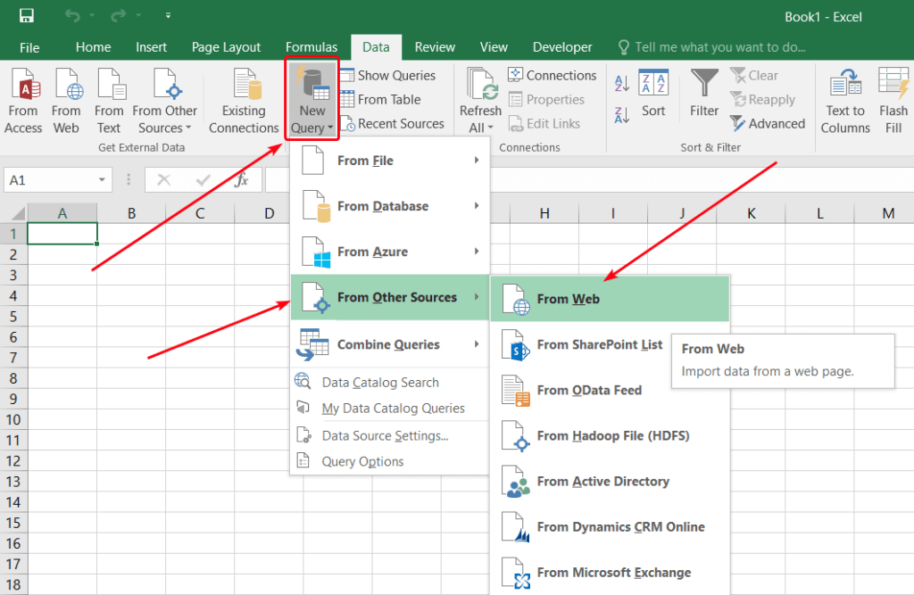
- Enter the web page URL and click OK:

Excel will look for tables on the page.
- In the Navigator window that opens, select the table that you want to import:

Use the Select multiple items checkbox if you want to import several tables. Click Load when you are ready to start the import.
- Excel will insert the imported table into the current worksheet. You can refresh data by clicking the refresh button in the Workbook Queries task pane:

How to automatically import live data into Excel
Data is relevant as long as it’s fresh. If you need to update the information frequently to keep it up-to-date, manual data import will bring nothing but pain.
Thankfully, many websites provide REST API for accessing their data. Sometimes you have to pay for API access, sometimes it’s free. You need to make a request to get the data. The details on making requests can be found in the API reference of the data provider. API responses usually contain data in JSON format. There are free services that allow you to import JSON data to Excel. The best ones will even make API requests for you. Let’s see how you can use Coupler.io for such tasks.
Coupler.io is a data integration solution for importing data into Excel from different apps. You can load records from Shopify, HubSpot, Pipedrive, and many other sources. In addition to Excel, you can use Google Sheets or BigQuery as a destination for your data.
- Sign in to Coupler.io with your Microsoft account.
- Go to Importers and click Add new importer.
- Select JSON as Source, and provide the request URL with your API key (if required):

Refer to the data provider documentation for details on available requests and how you can obtain an API key.
- Specify API call parameters, as described in the API documentation. The only required parameter is HTTP method, which will be ‘GET’ in most cases.
- In Destination, select Microsoft Excel:

- Connect to your Microsoft Office account, and then select an existing workbook for import. You can specify an existing sheet or create a new one by typing its name:

- Toggle the Automatic data refresh switch to set up the schedule for automatic data updates. When you are done with settings, click Save and Run:

Synchronizing the spreadsheets
How to sync data between Excel files
If you want to transfer data from one Excel workbook to another, copy-pasting is a good option. But that will not work if you want to keep the data up-to-date with the other file. There are several ways to sync data between Excel files.
You can use formulas for that. To fill a cell with data from another Excel workbook:
- Make sure that the other workbook is open.
- Select the cell to sync, then click the Formula Bar and type
=.

- Switch to the other workbook, click the cell that you want to import data from, and press Enter.
Excel will switch you back to the first workbook and fill the cell with the synced data. If the content of the cell in the other workbook changes, the synced cell will be updated.
If you see #REF! in the synced cell, it means that the other workbook is not open. Open it to enable data synchronization. Try another method if you are not comfortable with the formula bar.
- In the source file, i.e. the workbook that you want to import data from, select the cell, and then click Copy or press
Ctrl-C:

- Switch to the target workbook, select the cell, and then select Paste > Other Paste Options > Paste Link.
The formula for that cell will be filled with the link to the source cell in the other workbook.
There are many other options for syncing Excel data that you can learn in our guide on linking Excel files.
Besides the standard Excel features, there are online tools that allow you to import data from Excel to Excel, and let you synchronize your data in a more flexible way.
How to import data from Google Sheets to Excel
Google Sheets is almost as powerful as Excel in terms of data processing. But certain very important features are still available only in Excel. If you need these functions, you can transfer your data in several ways.
Import data from Google Sheets to Excel automatically
First of all, try using Coupler.io. It is an online tool that can import data from Google Sheets to Excel.
- Sign in to your Coupler.io account and click Add New in the Importers section.
- Select Google Sheets as Source, click Connect, and sign in to your Google account:
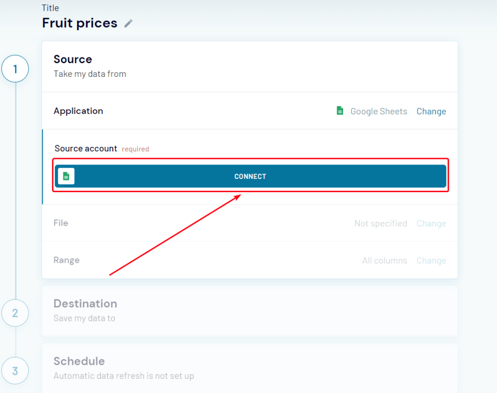
- Select the workbook and the sheet that you would like to export data from:

- Select the range of cells, or skip this step to export all the data.
- In Destination, select Microsoft Excel, click Continue, and then sign in to your Microsoft account.
- Select an existing workbook and the worksheet. If you want to create a new worksheet, just type its name:
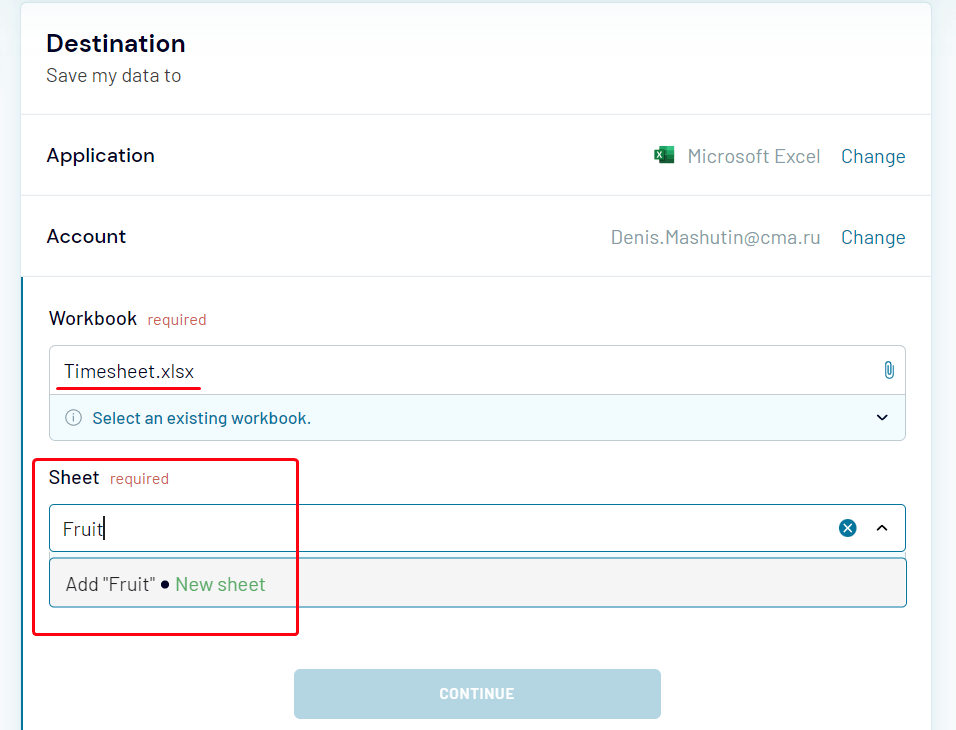
- Specify the cell address or keep the default ‘A1’ value.
- Specify the import mode. The default option is ‘Replace’.
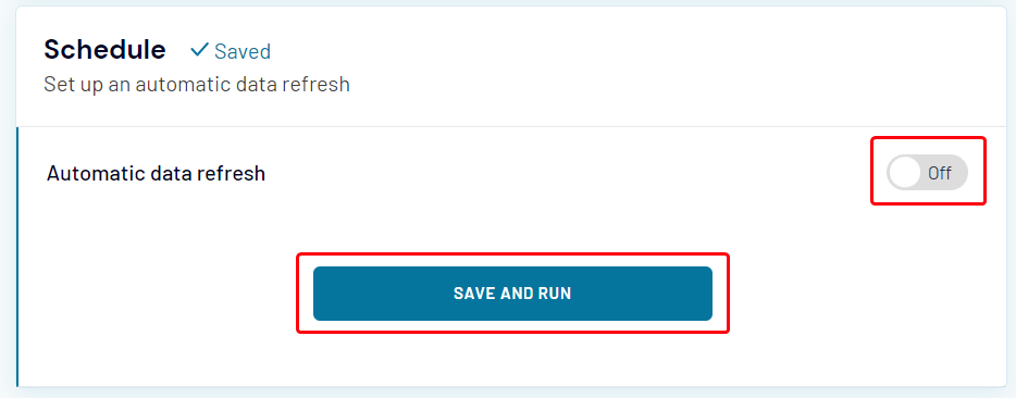
- Now you can click Save and Run to start the import immediately.
Or you can toggle Automatic data refresh to configure automatic data updates:
Import data from Google Sheets to Excel as HTML
The second option is to use the built-in data import feature of Excel:
- In your Google spreadsheet, go to File > Share > Publish to web:
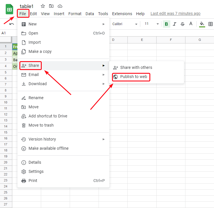
- Select the sheet that contains the table, and specify Comma-separated values (.csv).
If you want the data in Excel to be updated when the Google sheet is changed, select the Automatically republish when changes are made checkbox:

- Press
Ctrl-Cto copy the link. - Go to your Excel workbook and perform the steps described in the section about importing data from HTML above.
If you choose the second option, keep in mind that your data will become accessible by others. If the information is confidential or sensitive, using Coupler.io is preferred.
Importing data from other sources
How to import data from SQL server to Excel
If your data is stored in databases at an SQL server, the simplest way to make it accessible to a wide spectrum of users is to export it to Excel. You can use the native Excel query function.
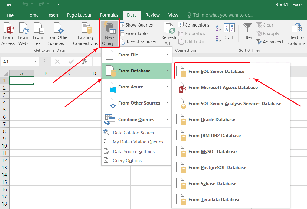
- In the Data tab, select New Query > From Database > From SQL Server Database:
- Specify the name of the server and the database (or you will be able to specify it later):

You can also provide an SQL statement to narrow the range of exported data.
- Choose to use your current window credentials to access the database, or provide the username and the password. Click Connect.
- In the next window, select the database and tables that you want to export.
- Select the name for the new data connection file, and then click Finish.
- In the next window, you can select where to insert the imported data. Select Existing worksheet and provide the cell address, if needed.
The data will be imported and pasted into the worksheet.
If you use SQL Server Management Studio (SSMS), there is a feature for exporting data to various destinations, including Excel spreadsheets.
- In Object Explorer, right-click the database with the source data, and then select Tasks > Export Data.
- In the SQL Server Import and Export Wizard window that opens, click Next.
- Select SQL Server Native Client 11.0 in the Data source drop-down box.
- Select Use Windows Authentication in the Authentication area, and then click Next.
- In the Choose a destination window, specify Microsoft Excel as the destination, browse to the target file in the Excel file path, and select the output file format.
- In the next window, you can choose to write a query for data export. If you want to copy the tables without changes, just click Next.
- The list of tables available for export will be displayed. Select the tables that you want to export. In the Destination column, you can specify the name of the worksheet for each table.
- In the Save and Run Package window, select Run immediately and click Next.
- Make sure that all parameters are correct, and then click Finish.
The selected data will be exported to the Excel workbook. When the wizard finishes all the tasks, click Close.
How to import data from a text file to Excel
The tables can also be stored in plain text. Such files are similar to regular text files with the only exception that commas have a special function there — they separate cells from each other. The format is called CSV — comma-separated values.
Excel can open .csv files directly. The content of such a file will be rendered as a table. If you edit a CSV file in Excel and then try to save it, you will see the following warning:

Click Yes if you want to continue using this file as CSV in the future. If you click No, the Save as dialogue will be opened, where you will be able to select the format and the destination for the file.
There are other delimiters that can be used to store tables in text format: tabs, pipes (‘|’), spaces, semicolons, etc. To open such files with Excel, instead of trying to open them directly, use the Power Query function.
- Go to Data > New Query > From File > From Text.
- Select the text file and click Import.
- The Query Editor window will open. Make sure that the table looks good and click Close & Load:

The imported table will be inserted into your current worksheet.
How to import data to Excel from PDF
If your tables are in PDF, but you want them in Excel, you can try to import them.
- Go to the Data tab, and then select New Query > From File > From PDF.
- Select the tables that you want to import in the Navigator window, and then click Load.
The tables will be extracted from PDF and pasted into your Excel workbook. If you don’t have the From PDF option on the menu, you can use the following workaround to import data from PDF into Excel:
- Copy the table text in the PDF file by selecting it and pressing
Ctrl-C. - Open Microsoft Word and press
Ctrl-V. - Check if Word managed to render the text data correctly:
- Press
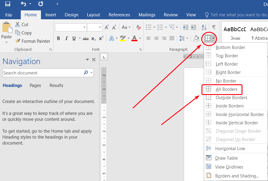
Ctrl-Ato select everything. - On the Home tab, click the table menu, and then select All borders:
- Press
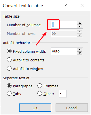
- If the table looks good, proceed to the final step. Otherwise, go to the Insert tab, and then select Table > Convert Text to Table:

- Specify the number of columns in the original table, and then click OK:
- Copy the entire table, go to Excel, and press
Ctrl-V.
The table will be inserted into the current worksheet. If you opt for this workaround, no automatic data synchronization will be available.
Discover many other sources for importing data to Excel
Excel provides you with many powerful features for data processing. You can bring virtually any data to Excel by importing it from various sources. If you didn’t find a good solution in this article, discover other Microsoft Excel integrations to pick what fits your needs best.
-

Lead Analytics Engineer at Railsware and Coupler.io. I make data accessible and useful for everyone in a team. During the last 7 years, I built dashboards, analyzed user journeys, and even caught criminals 🕵🏿♀️ Besides data, I also like doing yoga, cooking, and hiking 🤗

Back to Blog
Focus on your business
goals while we take care of your data!
Try Coupler.io
Importing live data into a Google Sheet or Excel spreadsheet might seem like a daunting task, but it’s easier than you think…
If you’re reading this you probably know spreadsheets are a useful way to aggregate, tidy and analyse data. But what you probably don’t know is that with some simple techniques and plugins, any humble spreadsheet can be transformed into an incredibly powerful, automated, data-gathering machine that can save you or your team hours of manual input.
In this post we look at four different ways to get almost any data into a spreadsheet.
How to get data into a spreadsheet
1. Manual input
Wait, aren’t we supposed to be looking at ways to import live data into a spreadsheet automatically?
Well, yes, but adding data into a spreadsheet by hand shouldn’t be dismissed entirely. Although it might seem inefficient, there are scenarios where this is the best or only option for getting data into a spreadsheet:
- If you’re working with small set of data on a one-off basis
- If your data doesn’t update frequently
- If the data sources you’re working with don’t allow data to be exported
- As a quick proof of concept that could be automated later
In addition, manually adding data to a spreadsheet can be made more efficient through outsourcing to a virtual assistant. Sites like Upwork, Freelancer.com and Fiverr make it quick and easy to find talented individuals who can help with large or repetitive data entry tasks. But we’ll save that for another post.
2. Use a third-party data import tool
A number of services, add-ons and tools specialize in getting data from a variety of sources into Google Sheets and Excel spreadsheets.
One of our favourites is Supermetrics — a flexible add-on for Google Sheets and Excel that lets you easily pull in data from many different tools, with a particular focus on marketing data.
For each data source you connect to Supermetrics, you can access a comprehensive range of metrics, data and information to bring in to your spreadsheet, and it’s even possible to schedule automatic importing of new data so your spreadsheet always contains up-to-date data.
Data sources that Supermetrics supports include: Adobe Analytics, AdRoll, Google BigQuery, Google Search Console, Moz, Optimizely, Pinterest, SEMrush, and more.
Here’s a quick overview of how to import data into Google Sheets using Supermetrics:
- Install the Supermetrics add-on in the G Suite Marketplace
- In a Google Sheet, select Add-ons from the main menu, then Supermetrics > Launch
- Select a data source from the list of available sources and authorize it to share data with Supermetrics
- Build a query using the options available and then click Get Data to Table
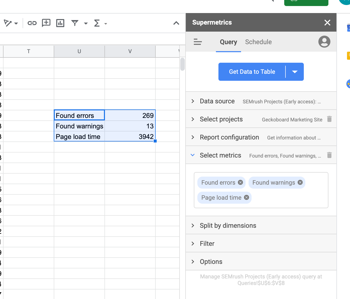
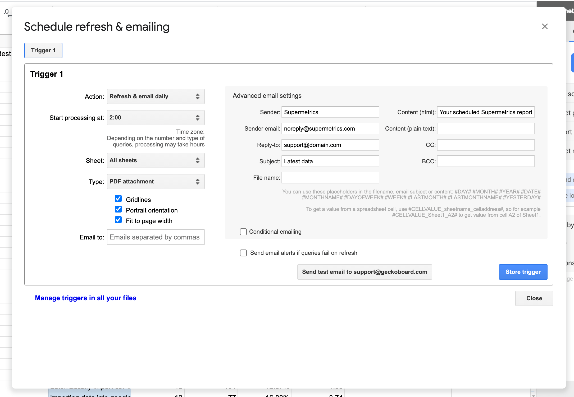
Once you’re happy with the query you’ve built, you can then schedule it to re-run weekly, daily or even hourly which will fetch new data and add it to your spreadsheet. You can also have Supermetrics send a snapshot of your updated spreadsheet to an email address.
There are a range of similar plugins and add-ons that have their own strengths. Some of the ones we like include:
- Make (formerly Integromat): allows for complex workflows, filtering and blending of data before data is sent to a Google Sheet or Excel spreadsheet. Data sources supported include JSON, CSV files, RSS and XML feeds, and hundreds of third party APIs.
- Zapier: A huge range of data sources (5000+) that can manipulate or add data to a spreadsheet automatically
- Google Analytics’ Google Sheets add-on: Import detailed information from Google Analytics into a Google Sheet
- Adobe’s Report Builder (Excel): If you use Adobe Analytics, Report Builder is a plugin that enables you to extract your Analytics data from Adobe into Excel.

3. Import Functions (Google Sheets)
An entire library of functions in Google Sheets allows you to achieve powerful results using simple formulae.
Google Sheets offers five different import functions (listed below) that allow it to pull data into your spreadsheet from a variety of sources including XML, HTML, RSS and CSV — perfect for importing lists of blog posts, tweaks, product inventories or data from another service.
Here are the specific functions along with the type of data they collect:
IMPORTDATA(url)
Imports data at a given url in .csv (comma-separated value) or .tsv (tab-separated value) format.
See more detail about using Google Sheets’ IMPORTDATA function to display CSV data here: Using Google Sheets’ ImportData function
IMPORTHTML(url, query, index)
Imports data from a table or list within an HTML webpage.
See more detail about using Google Sheets’ IMPORTHTML function here: Using Google Sheets’ ImportHTML function
IMPORTXML(url, xpath_query)
Imports data from any of various structured data types including XML, HTML, CSV, TSV, and RSS and ATOM XML feeds.
See more detail about using Google Sheets’ IMPORTXML function here: Using Google Sheets’ ImportXML function
IMPORTFEED(url, query, headers, num_items)
Imports a RSS or ATOM feed.
IMPORTRANGE(spreadsheet_key, range_string)
Imports a range of cells from a specified spreadsheet.
Using these functions, you can easily scrape data from web pages, feeds and files. Also, a built-in finance function enables you to pull back market data.
Other useful Google Sheets functions
- Creating a Countdown Timer using Google Sheets
- GOOGLEFINANCE function to display market data
4. Scripting (Google Sheets)
Scripting (or in non-technical terms — writing a short bit of custom code) can be a powerful way to get data into Google Sheets. It’s basically an easier way to write large spreadsheet formulas and functions.
Google Apps Script is a cloud-based scripting language that provides easy ways to automate tasks across Google products and other services.
Google Apps scripts are extremely flexible, and can be automated using a variety of triggers, and although they need more technical knowledge to write and set up, an active community is on hand to offer guidance and help.
At Geckoboard, we use Discourse to power our Community we use Google Apps Scripts to fetch data from Discourse and add it to a spreadsheet, which we then visualize on a live dashboard to see how key metrics are performing.
Here are the steps we took to pull data from our Community to Google Sheets, to a dashboard:
- Created a new Google Sheets Spreadsheet
- Created a new script for our Spreadsheet (Tools > Script editor) and copy and pasted chrislkeller’s ImportJSON functions (to be able to import the output of Discourse’s API which is JSON).
- Looked in Discourse’s API documentation for a call that returned the latest topics created in the Community
- Added a new function in our script to call the endpoint identified on step 3 and update cell A1 with the response
- Finally, added a trigger to run the function myFunction every hour.
- Used Google Sheets standard functions to identify the rows containing topics created Today and count them.
- Used Geckoboard’s spreadsheets integration to get the data onto a dashboard (more about this in the section below).
Google offers a variety of resources to help you make the most of Google Sheets using Google Apps Scripts. You might find some of their examples useful to get your data into Google Sheets.
Beyond spreadsheets: visualizing and sharing your data
Want to take your spreadsheet game even further? Now that you’ve imported data from various sources into your Google Sheets and Excel spreadsheets, you can easily visualize and share this information using a dashboard.

Learn more about this Excel dashboard example here.
The example above contains a variety of visualizations, which can be powered either by Google Sheets or an Excel spreadsheet, which updates automatically to show up-to-the-minute data.
Here’s how it works
- Create your spreadsheet in Google Sheets or Excel (importing data from via the steps mentioned earlier in this post)
- Sign up for a free Geckoboard account
- Select ‘Add dashboard’, then ‘Add widget’
- Pick the ‘Spreadsheet’ integration from the list of data sources.
- Select your data and choose a visualization
- Build out your dashboard by adding more visualizations
Watch this in action in the video below!
Let us know on Twitter if you’ve found any other useful or interesting ways to get data into a spreadsheet.
Originally published on 23rd February 2016, updated on 6th October 2022
Share your goals, metrics, and data on a live dashboard
Geckoboard is the easiest way to make key information visible for your team.
Learn how
Содержание
- Как это работает
- Подключаем внешние данные из интернет
- Импорт внешних данных Excel 2010
- Отличите нового и старого мастера импорта
- Пример работы функции БИЗВЛЕЧЬ при выборке данных из таблицы Excel
- Примеры использования функции БИЗВЛЕЧЬ в Excel
- Тип данных: Числовые значения MS Excel
- Классификация типов данных
- Текстовые значения
- Дата и время
- Логические данные
- Разновидности типов данных
- Число
- Текст
- Ошибки
- Подключение к внешним данным
- Подключение к базе данных
- Импорт данных из базы данных Microsoft Access
- Импорт данных с веб-страницы
- Копировать-вставить данные из Интернета
- Импорт данных из текстового файла
- Импорт данных из другой книги
- Импорт данных из других источников
- Задача для получения данных в Excel
Как это работает
Инструменты для импорта расположены во вкладке меню «Данные». 
Если подключение отключено, перейдите: 
Далее: 
На вкладке «Центр управления» перейдите: 
Подключаем внешние данные из интернет
В Excel 2013 и более поздних версиях, по умолчанию для импорта информации из внешних источников используется надстройка Power Query. Как это работает? Перейдите: 
Пропишите адрес сайта, с которого импортируются данные: 
Выберите что отобразится, нажмите кнопку «Загрузить». 
Информация подгрузится в лист Excel. Работайте с ними как с простым документом: используйте формулы графики, сводные таблицы. 
Для обновления нажмите ПКМ по таблице: 
Или: 
Импорт внешних данных Excel 2010
Перейдите: 
В новом окне пропишите адрес сайта. Получите информацию из областей страницы, где проставлены желтые ярлыки. Отметьте их мышкой, нажмите «Импорт». 
Отметьте пункт «Обновление». Тогда внешняя информация обновится автоматически. 
Отличите нового и старого мастера импорта
Преимущества Power Query:
- Поддерживается работа с большим числом страниц;
- Промежуточная обработка информации перед загрузкой на лист;
- Информация импортируется быстрее.
Как создать базу данных в Excel? Базой данных в программе Excel считается таблица, которая была создана с учетом определенных требований:
- Заголовки таблицы должны находиться в первой строке.
- Любая последующая строка должна содержать хотя бы одну непустую ячейку.
- Объединения ячеек в любых строках запрещены.
- Для каждой ячейки каждого столбца должен быть определен единый тип хранящихся данных.
- Диапазон базы данных должен быть отформатирован в качестве списка и иметь свое имя.
Таким образом, практически любая таблица в Excel может быть преобразована в базу данных. Ее строки являются записями, а столбцы – полями данных.
Функция БИЗВЛЕЧЬ хорошо работает с корректно отформатированными таблицами.
Примеры использования функции БИЗВЛЕЧЬ в Excel
Пример 1. В таблице, которую можно рассматривать как БД, содержатся данные о различных моделях смартфонов. Найти название бренда смартфона, который содержит процессор с минимальным числом ядер.
Вид таблиц данных и критериев:

В ячейке B2 запишем условие отбора данных следующим способом:
=МИН(СТОЛБЕЦ(B1))
Данный вариант записи позволяет унифицировать критерий для поиска данных в изменяющейся таблице (если число записей будет увеличиваться или уменьшаться со временем).
В результате получим следующее:

В ячейке A4 запишем следующую формулу:
Описание аргументов:
- A8:F15 – диапазон ячеек, в которых хранится БД;
- 1 – числовое указание номера поля (столбца), из которого будет выводиться значение (необходимо вывести Бренд);
- A2:F3 – диапазон ячеек, в которых хранится таблица критериев.
Результат вычислений:

При изменении значений в таблице параметров условий мы будем автоматически получать выборку соответственных им результатов.
Тип данных: Числовые значения MS Excel
Числовые значения, в отличие от текстовых, можно и складывать и умножать и вообще, применять к ним весь богатый арсенал экселевских средств по обработке данных. После ввода в пустую ячейку MS Excel, числовые значения выравнивается по правой границе ячейки.
Фактически, к числовым типам данных относятся:
- сами числа (и целые и дробные и отрицательные и даже записанные в виде процентов)
- дата и время
Несколько особенностей числовых типов данных
Если введенное число не помещается в ячейку, то оно будет представлено в экспоненциальной форму представления, здорово пугающей неподготовленных пользователей. Например, гигантское число 4353453453453450 х 54545 в ячейку будет записано в виде 2,37459Е+20. Но, как правило в «жизни» появление «странных чисел» в ячейках excel свидетельствует о простой ошибке.

Если число или дата не помещается в ячейку целиком, вместо цифр в ней появляются символы ###. В этом случае «лечение» ещё более простое — нужно просто увеличить ширину столбца таблицы.
Иногда есть необходимостью записать число как текст, например в случае записи всевозможных артикулов товаров и т.п. дело в том, что если вы запишите 000335 в ячейку, Excel посчитав это значение числом, сразу же удалит нули, превратив артикул в 335. Чтобы этого не произошло, просто поместите число в кавычки — это будет сигналом для Excel, что содержимое ячейки надо воспринимать как текст, то есть выводить также, как его ввел пользователь. Естественно, производить с таким числом математических операций нельзя.
Что представляет собой дата в MS Excel?
Если с числами все более-менее понятно, то даты имеют несколько особенностей, о которых стоит упомянуть. Для начала, что такое «дата» с точки зрения MS Excel? На самом деле все не так уж и просто.
Дата в Excel — это число дней, отсчитанных до сегодняшнего дня, от некой начальной даты. По умолчанию этой начальной датой считается 1 января 1900 года.
А что же текущее время? Ещё интереснее — за точку отсчета каждых суток берется 00:00:00, которое представляется как 1. А дальше, эта единичка уменьшается, по мере того как уменьшается оставшееся в сутках время. Например 12.00 дня это с точки зрения MS Excel 0,5 (прошла половина суток), а 18.00 — 0,25 (прошли 3 четверти суток).
В итоге, дата 17 июня 2019 года, 12:30, «языком экселя» выглядит как 43633 (17.06.19) + 0,52 (12:30), то есть число 43633,52.

Как превратить число в текст? Поместите его в кавычки!
Классификация типов данных
Тип данных — это характеристика информации, хранимой на листе. На основе этой характеристики программа определяет, каким образом обрабатывать то или иное значение.
Типы данных делятся на две большие группы: константы и формулы. Отличие между ними состоит в том, что формулы выводят значение в ячейку, которое может изменяться в зависимости от того, как будут изменяться аргументы в других ячейках. Константы – это постоянные значения, которые не меняются.
В свою очередь константы делятся на пять групп:
- Текст;
- Числовые данные;
- Дата и время;
- Логические данные;
- Ошибочные значения.
Текстовые значения
Текстовый тип содержит символьные данные и не рассматривается Excel, как объект математических вычислений. Это информация в первую очередь для пользователя, а не для программы. Текстом могут являться любые символы, включая цифры, если они соответствующим образом отформатированы. В языке DAX этот вид данных относится к строчным значениям. Максимальная длина текста составляет 268435456 символов в одной ячейке.
Для ввода символьного выражения нужно выделить ячейку текстового или общего формата, в которой оно будет храниться, и набрать текст с клавиатуры. Если длина текстового выражения выходит за визуальные границы ячейки, то оно накладывается поверх соседних, хотя физически продолжает храниться в исходной ячейке.

Дата и время
Ещё одним типом данных является формат времени и даты. Это как раз тот случай, когда типы данных и форматы совпадают. Он характеризуется тем, что с его помощью можно указывать на листе и проводить расчеты с датами и временем. Примечательно, что при вычислениях этот тип данных принимает сутки за единицу. Причем это касается не только дат, но и времени. Например, 12:30 рассматривается программой, как 0,52083 суток, а уже потом выводится в ячейку в привычном для пользователя виде.
Существует несколько видов форматирования для времени:
- ч:мм:сс;
- ч:мм;
- ч:мм:сс AM/PM;
- ч:мм AM/PM и др.

Аналогичная ситуация обстоит и с датами:
- ДД.ММ.ГГГГ;
- ДД.МММ
- МММ.ГГ и др.

Есть и комбинированные форматы даты и времени, например ДД:ММ:ГГГГ ч:мм.

Также нужно учесть, что программа отображает как даты только значения, начиная с 01.01.1900.
Логические данные
Довольно интересным является тип логических данных. Он оперирует всего двумя значениями: «ИСТИНА» и «ЛОЖЬ». Если утрировать, то это означает «событие настало» и «событие не настало». Функции, обрабатывая содержимое ячеек, которые содержат логические данные, производят те или иные вычисления.

Разновидности типов данных
Выделяются две большие группы типов данных:
- константы – неизменные значения;
- формулы – значения, которые меняются в зависимости от изменения других.
В группу “константы” входят следующие типы данных:
- числа;
- текст;
- дата и время;
- логические данные;
- ошибки.
Число
Этот тип данных применяется в различных расчетах. Как следует из названия, здесь предполагается работа с числами, и для которых может быть задан один из следующих форматов ячеек:
- числовой;
- денежный;
- финансовый;
- процентный;
- дробный;
- экспоненциальный.
Формат ячейки можно задать двумя способами:
- Во вкладке “Главная” в группе инструментов “Число” нажимаем по стрелке рядом с текущим значением и в раскрывшемся списке выбираем нужный вариант.

- В окне форматирования (вкладка “Число”), в которое можно попасть через контекстное меню ячейки.


Для каждого из форматов, перечисленных выше (за исключением дробного), можно задать количество знаков после запятой, а для числового – к тому же, включить разделитель групп разрядов.

Чтобы ввести значение в ячейку, достаточно просто выделить ее (с нужным форматом) и набрать с помощью клавиш на клавиатуре нужные символы (либо вставить ранее скопированные данные из буфера обмена). Или можно выделить ячейку, после чего ввести нужные символы в строке формул.
Также можно поступить наоборот – сначала ввести значение в нужной ячейке, а формат поменять после.
Текст
Данный тип данных не предназначен для выполнения расчетов и носит исключительно информационный характер. В качестве текстового значения могут использоваться любые знаки, цифры и т.д.
Ввод текстовой информации происходит таким же образом, как и числовой. Если текст не помещается в рамках выбранной ячейки, он будет перекрывать соседние (если они пустые).

Ошибки
В некоторых случаях пользователь может видеть в Excel ошибки, которые бывают следующих видов:

- #ДЕЛ/О! – результат деления на число 0
- #Н/Д – введены недопустимые данные;
- #ЗНАЧ! – использование неправильного вида аргумента в функции;
- #ЧИСЛО! – неверное числовое значение;
- #ССЫЛКА! – удалена ячейка, на которую ссылалась формула;
- #ИМЯ? – неправильное имя в формуле;
- #ПУСТО! – неправильно указан адрес дапазона.
Подключение к внешним данным
Вы можете получить доступ к внешним источникам через вкладку Данные, группу Получить и преобразовать данные. Подключения к данным хранятся вместе с книгой, и вы можете просмотреть их, выбрав пункт Данные –> Запросы и подключения.
Подключение к данным может быть отключено на вашем компьютере. Для подключения данных пройдите по меню Файл –> Параметры –> Центр управления безопасностью –> Параметры центра управления безопасностью –> Внешнее содержимое. Установите переключатель на одну из опций: включить все подключения к данным (не рекомендуется) или запрос на подключение к данным.

Настройка доступа к внешним данным; чтобы увеличить изображение кликните на нем правой кнопкой мыши и выберите Открыть картинку в новой вкладке
Подробнее о подключении к внешним источникам данных см. Кен Пульс и Мигель Эскобар. Язык М для Power Query. При использовании таблиц, подключенных к данным можно переставлять и удалять столбцы, не изменяя запрос. Excel продолжает сопоставлять запрошенные данные с правильными столбцами. Однако ширина столбцов обычно автоматически устанавливается при обновлении. Чтобы запретить Excel автоматически устанавливать ширину столбцов Таблицы при обновлении, щелкните правой кнопкой мыши в любом месте Таблицы и пройдите по меню Конструктор –> Данные из внешней таблицы –> Свойства, а затем снимите флажок Задать ширину столбца.

Свойства Таблицы, подключенной к внешним данным
Подключение к базе данных
Для подключения к базе данных SQL Server выберите Данные –> Получить данные –> Из базы данных –> Из базы данных SQL Server. Появится мастер подключения к данным, предлагающий элементы управления для указания имени сервера и типа входа, который будет использоваться для открытия соединения. Обратитесь к своему администратору SQL Server или ИТ-администратору, чтобы узнать, как ввести учетные данные для входа.

Подключение к базе данных SQL Server
При импорте данных в книгу Excel их можно загрузить в модель данных, предоставив доступ к ним другим инструментам анализа, таким как Power Pivot.
Существует много различных типов доступных источников данных, и иногда шаблоны соединений по умолчанию, представленные Excel, не работают.
Импорт данных из базы данных Microsoft Access
Мы научимся импортировать данные из базы данных MS Access. Следуйте инструкциям ниже
Шаг 1 – Откройте новую пустую книгу в Excel.
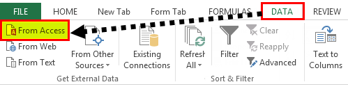
Шаг 2 – Перейдите на вкладку ДАННЫЕ на ленте.
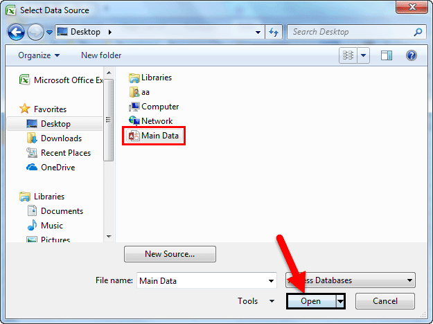
Шаг 3 – Нажмите « Доступ» в группе «Получить внешние данные». Откроется диалоговое окно « Выбор источника данных ».

Шаг 4 – Выберите файл базы данных Access, который вы хотите импортировать. Файлы базы данных Access будут иметь расширение .accdb.

Откроется диалоговое окно «Выбор таблицы», в котором отображаются таблицы, найденные в базе данных Access. Вы можете импортировать все таблицы в базе данных одновременно или импортировать только выбранные таблицы на основе ваших потребностей анализа данных.

Шаг 5 – Установите флажок Включить выбор нескольких таблиц и выберите все таблицы.

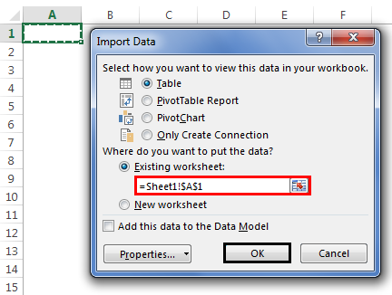
Шаг 6 – Нажмите ОК. Откроется диалоговое окно « Импорт данных ».

Как вы заметили, у вас есть следующие опции для просмотра данных, которые вы импортируете в свою рабочую книгу:
- Таблица
- Отчет сводной таблицы
- PivotChart
- Power View Report
У вас также есть возможность – только создать соединение . Далее отчет по сводной таблице выбран по умолчанию.
Excel также дает вам возможность поместить данные в вашу книгу –
- Существующий лист
- Новый лист
Вы найдете еще один флажок, который установлен и отключен. Добавьте эти данные в модель данных . Каждый раз, когда вы импортируете таблицы данных в свою книгу, они автоматически добавляются в модель данных в вашей книге. Вы узнаете больше о модели данных в следующих главах.
Вы можете попробовать каждый из вариантов, чтобы просмотреть импортируемые данные и проверить, как эти данные отображаются в вашей рабочей книге.
-
Если вы выберете « Таблица» , опция «Существующая рабочая таблица» будет отключена, будет выбрана опция « Новая рабочая таблица», и Excel создаст столько таблиц, сколько будет импортировано таблиц из базы данных. Таблицы Excel отображаются в этих таблицах.
-
Если вы выберете Отчет сводной таблицы , Excel импортирует таблицы в рабочую книгу и создаст пустую сводную таблицу для анализа данных в импортированных таблицах. У вас есть возможность создать сводную таблицу на существующем листе или новом листе.
Таблицы Excel для импортированных таблиц данных не будут отображаться в книге. Однако вы найдете все таблицы данных в списке полей сводной таблицы вместе с полями в каждой таблице.
-
Если вы выберете PivotChart , Excel импортирует таблицы в рабочую книгу и создаст пустую PivotChart для отображения данных в импортированных таблицах. У вас есть возможность создать сводную диаграмму на существующем или новом листе.
Таблицы Excel для импортированных таблиц данных не будут отображаться в книге. Однако вы найдете все таблицы данных в списке полей PivotChart вместе с полями в каждой таблице.
-
Если вы выберите Power View Report , Excel импортирует таблицы в рабочую книгу и создаст Power View Report в новой рабочей таблице. В последующих главах вы узнаете, как использовать отчеты Power View для анализа данных.
Таблицы Excel для импортированных таблиц данных не будут отображаться в книге. Однако вы найдете все таблицы данных в списке полей Power View Report вместе с полями в каждой таблице.
-
Если вы выберете опцию – Только создать соединение , между базой данных и вашей книгой будет установлено соединение для передачи данных. Таблицы или отчеты не отображаются в книге. Однако импортированные таблицы по умолчанию добавляются в модель данных в вашей книге.
Вам необходимо выбрать любой из этих параметров в зависимости от вашего намерения импортировать данные для анализа данных. Как вы заметили выше, независимо от выбранной вами опции, данные импортируются и добавляются в модель данных в вашей рабочей книге.
Если вы выберете « Таблица» , опция «Существующая рабочая таблица» будет отключена, будет выбрана опция « Новая рабочая таблица», и Excel создаст столько таблиц, сколько будет импортировано таблиц из базы данных. Таблицы Excel отображаются в этих таблицах.
Если вы выберете Отчет сводной таблицы , Excel импортирует таблицы в рабочую книгу и создаст пустую сводную таблицу для анализа данных в импортированных таблицах. У вас есть возможность создать сводную таблицу на существующем листе или новом листе.
Таблицы Excel для импортированных таблиц данных не будут отображаться в книге. Однако вы найдете все таблицы данных в списке полей сводной таблицы вместе с полями в каждой таблице.
Если вы выберете PivotChart , Excel импортирует таблицы в рабочую книгу и создаст пустую PivotChart для отображения данных в импортированных таблицах. У вас есть возможность создать сводную диаграмму на существующем или новом листе.
Таблицы Excel для импортированных таблиц данных не будут отображаться в книге. Однако вы найдете все таблицы данных в списке полей PivotChart вместе с полями в каждой таблице.
Если вы выберите Power View Report , Excel импортирует таблицы в рабочую книгу и создаст Power View Report в новой рабочей таблице. В последующих главах вы узнаете, как использовать отчеты Power View для анализа данных.
Таблицы Excel для импортированных таблиц данных не будут отображаться в книге. Однако вы найдете все таблицы данных в списке полей Power View Report вместе с полями в каждой таблице.
Если вы выберете опцию – Только создать соединение , между базой данных и вашей книгой будет установлено соединение для передачи данных. Таблицы или отчеты не отображаются в книге. Однако импортированные таблицы по умолчанию добавляются в модель данных в вашей книге.
Вам необходимо выбрать любой из этих параметров в зависимости от вашего намерения импортировать данные для анализа данных. Как вы заметили выше, независимо от выбранной вами опции, данные импортируются и добавляются в модель данных в вашей рабочей книге.
Импорт данных с веб-страницы
Иногда вам может понадобиться использовать данные, которые обновляются на веб-сайте. Вы можете импортировать данные из таблицы на веб-сайте в Excel.
Шаг 1 – Откройте новую пустую книгу в Excel.
Шаг 2 – Перейдите на вкладку ДАННЫЕ на ленте.
Шаг 3 – Нажмите « Из Интернета» в группе « Получить внешние данные ». Откроется диалоговое окно « Новый веб-запрос ».

Шаг 4 – Введите URL-адрес веб-сайта, с которого вы хотите импортировать данные, в поле рядом с адресом и нажмите «Перейти».

Шаг 5 – Данные на сайте появляются. Рядом с данными таблицы будут отображаться желтые значки со стрелками, которые можно импортировать.

Шаг 6 – Нажмите желтые значки, чтобы выбрать данные, которые вы хотите импортировать. Это превращает желтые значки в зеленые поля с галочкой, как показано на следующем снимке экрана.

Шаг 7 – Нажмите кнопку «Импорт» после того, как вы выбрали то, что вы хотите.

Откроется диалоговое окно « Импорт данных ».

Шаг 8 – Укажите, куда вы хотите поместить данные и нажмите Ok.
Шаг 9 – Организовать данные для дальнейшего анализа и / или представления.

Копировать-вставить данные из Интернета
Другой способ получения данных с веб-страницы – копирование и вставка необходимых данных.
Шаг 1 – Вставьте новый лист.
Шаг 2 – Скопируйте данные с веб-страницы и вставьте их на лист.
Шаг 3 – Создайте таблицу с вставленными данными.

Импорт данных из текстового файла
Если у вас есть данные в файлах .txt или .csv или .prn , вы можете импортировать данные из этих файлов, рассматривая их как текстовые файлы. Следуйте инструкциям ниже
Шаг 1 – Откройте новый лист в Excel.
Шаг 2 – Перейдите на вкладку ДАННЫЕ на ленте.
Шаг 3 – Нажмите « Из текста» в группе «Получить внешние данные». Откроется диалоговое окно « Импорт текстового файла ».

Вы можете видеть, что текстовые файлы с расширениями .prn, .txt и .csv принимаются.
Шаг 4 – Выберите файл. Имя выбранного файла появится в поле Имя файла. Кнопка «Открыть» изменится на кнопку «Импорт».

Шаг 5 – Нажмите кнопку «Импорт». Мастер импорта текста – появляется диалоговое окно « Шаг 1 из 3 ».
Шаг 6 – Выберите опцию «С разделителями», чтобы выбрать тип файла, и нажмите «Далее».

Откроется мастер импорта текста – шаг 2 из 3 .
Шаг 7 – В разделе «Разделители» выберите « Другое» .
Шаг 8 – В поле рядом с Другой введите | (Это разделитель в текстовом файле, который вы импортируете).
Шаг 9 – Нажмите Далее.

Откроется мастер импорта текста – шаг 3 из 3 .
Шаг 10 – В этом диалоговом окне вы можете установить формат данных столбца для каждого из столбцов.

Шаг 11. После завершения форматирования данных столбцов нажмите кнопку «Готово». Откроется диалоговое окно « Импорт данных ».

Вы увидите следующее –
-
Таблица выбрана для просмотра и отображается серым цветом. Таблица – единственный вариант просмотра, который у вас есть в этом случае.
-
Вы можете поместить данные либо в существующий рабочий лист, либо в новый рабочий лист.
-
Вы можете установить или не устанавливать флажок Добавить эти данные в модель данных.
-
Нажмите OK после того, как вы сделали выбор.
Таблица выбрана для просмотра и отображается серым цветом. Таблица – единственный вариант просмотра, который у вас есть в этом случае.
Вы можете поместить данные либо в существующий рабочий лист, либо в новый рабочий лист.
Вы можете установить или не устанавливать флажок Добавить эти данные в модель данных.
Нажмите OK после того, как вы сделали выбор.
Данные появятся на указанном вами листе. Вы импортировали данные из текстового файла в книгу Excel.
Импорт данных из другой книги
Возможно, вам придется использовать данные из другой книги Excel для анализа данных, но кто-то другой может поддерживать другую книгу.
Чтобы получать последние данные из другой книги, установите соединение данных с этой книгой.
Шаг 1 – Нажмите DATA> Соединения в группе Соединения на ленте.
Откроется диалоговое окно « Подключения к книге».

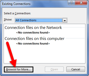
Шаг 2. Нажмите кнопку «Добавить» в диалоговом окне «Подключения к книге». Откроется диалоговое окно « Существующие подключения ».

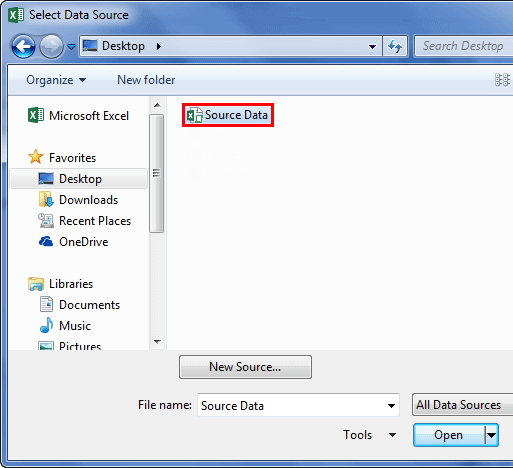
Шаг 3 – Нажмите кнопку Обзор для более … Откроется диалоговое окно « Выбор источника данных ».

Шаг 4 – Нажмите кнопку « Новый источник» . Откроется диалоговое окно мастера подключения к данным .

Шаг 5 – Выберите Other / Advanced в списке источников данных и нажмите Next. Откроется диалоговое окно «Свойства ссылки на данные».

Шаг 6 – Установите свойства канала передачи данных следующим образом –
-
Перейдите на вкладку « Соединение ».
-
Нажмите Использовать имя источника данных.
-
Нажмите стрелку вниз и выберите « Файлы Excel» в раскрывающемся списке.
-
Нажмите ОК.
Перейдите на вкладку « Соединение ».
Нажмите Использовать имя источника данных.
Нажмите стрелку вниз и выберите « Файлы Excel» в раскрывающемся списке.
Нажмите ОК.
Откроется диалоговое окно « Выбрать рабочую книгу ».

Шаг 7 – Найдите место, где у вас есть рабочая книга для импорта. Нажмите ОК.
Откроется диалоговое окно « Мастер подключения к данным » с выбором базы данных и таблицы.
Примечание. В этом случае Excel обрабатывает каждый рабочий лист, который импортируется, как таблицу. Имя таблицы будет именем рабочего листа. Таким образом, чтобы иметь значимые имена таблиц, назовите / переименуйте рабочие листы в зависимости от ситуации.

Шаг 8 – Нажмите Далее. Откроется диалоговое окно мастера подключения к данным с сохранением файла подключения к данным и завершением.

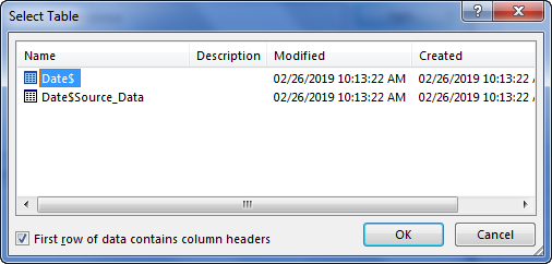
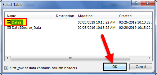
Шаг 9 – Нажмите кнопку Готово. Откроется диалоговое окно « Выбор таблицы ».

Как вы заметили, Name – это имя листа, которое импортируется как тип TABLE. Нажмите ОК.
Соединение данных с выбранной вами рабочей книгой будет установлено.
Импорт данных из других источников
Excel предоставляет вам возможность выбора различных других источников данных. Вы можете импортировать данные из них в несколько шагов.
Шаг 1 – Откройте новую пустую книгу в Excel.
Шаг 2 – Перейдите на вкладку ДАННЫЕ на ленте.
Шаг 3 – Нажмите Из других источников в группе Получить внешние данные.

Появляется выпадающий список с различными источниками данных.

Вы можете импортировать данные из любого из этих источников данных в Excel.
Задача для получения данных в Excel
И для того чтобы более понятно рассмотреть данную возможность, мы это будем делать как обычно на примере. Другими словами допустим, что нам надо выгрузить данные, одной таблицы, из базы SQL сервера, средствами Excel, т.е. без помощи вспомогательных инструментов, таких как Management Studio SQL сервера.
Примечание! Все действия мы будем делать, используя Excel 2010. SQL сервер у нас будет MS Sql 2008.
И для начала разберем исходные данные, допустим, есть база test, а в ней таблица test_table, данные которой нам нужно получить, для примера будут следующими:

Эти данные располагаются в таблице test_table базы test, их я получил с помощью простого SQL запроса select, который я выполнил в окне запросов Management Studio. И если Вы программист SQL сервера, то Вы можете выгрузить эти данные в Excel путем простого копирования (данные не большие), или используя средство импорта и экспорта MS Sql 2008.
Источники
- https://public-pc.com/podklyuchenie-vneshnih-dannyh-v-excel/
- https://exceltable.com/funkcii-excel/vyborka-iz-bazy-dannyh-bizvlech
- http://bussoft.ru/tablichnyiy-redaktor-excel/tipy-dannyh-v-redaktore-elektronnyh-tablicz-ms-excel.html
- https://lumpics.ru/data-types-in-excel/
- https://MicroExcel.ru/tipy-dannyh/
- https://baguzin.ru/wp/glava-8-rabota-s-vneshnimi-dannymi-v-tablitsah-excel/
- https://coderlessons.com/tutorials/bolshie-dannye-i-analitika/izuchite-analiz-dannykh-excel/import-dannykh-v-excel
- https://info-comp.ru/obucheniest/375-excel-get-data-from-sql-server.html
How to Import Data in Excel?
Importing the data from another file or another source file is often required in Excel. For example, sometimes people need data directly from very complicated servers, and sometimes we may need to import data from a text file or even from an Excel workbook.
If you are new to Excel data importing, then in this article, we will take a tour of importing data from text files, different Excel workbooks, and MS Access. Follow this article to learn the process involved in importing the data.
Table of contents
- How to Import Data in Excel?
- #1 – Import Data from Another Excel Workbook
- #2 – Import Data from MS Access to Excel
- #3 – Import Data from Text File to Excel
- Things to Remember
- Recommended Articles
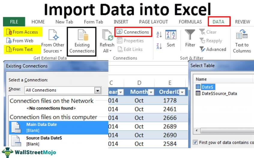
#1 – Import Data from Another Excel Workbook
You can download this Import Data Excel Template here – Import Data Excel Template
Let us start.
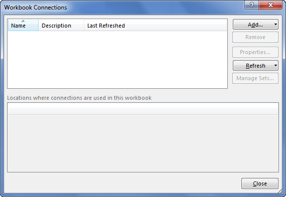
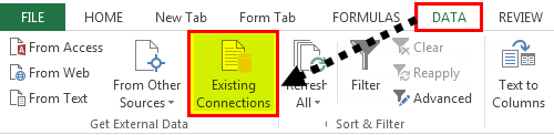
- First, we must go to the DATA tab. Then, under the DATA tab, click on Connections.

- As soon as we click on Connections, we may see the below window separately.

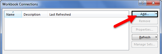
- Now, click on Add.

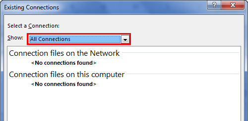
- It will open up a new window. In the below window, select All Connections.

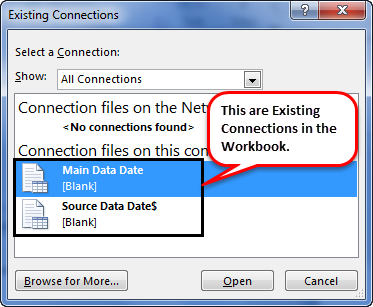
- If there are any connections in this workbook, it will show what those connections are here.

- Since we are connecting to a new workbook, click on Browse for more.

- In the below window, browse the file location. Then, click on Open.

- After clicking on Open, it shows the below window.

- Here, we need to select the required table to be imported to this workbook. Select the table and click on OK.
After clicking on OK, close the Workbook Connection window.
- Then, go to Existing Connections under the DATA tab.

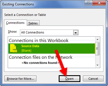
- Here, we will see all the existing connections. Select the connection we have just made and click on Open.

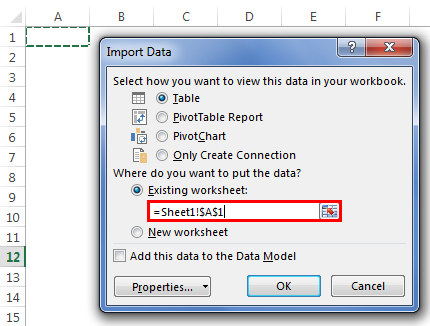
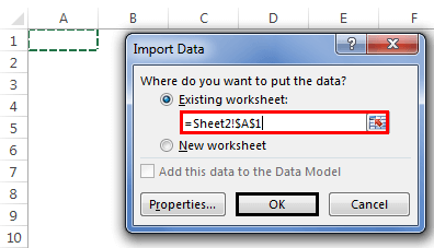
- Once we click on Open, it will ask us where to import the data. First, we need to select the cell reference here. Then, click on the OK button.

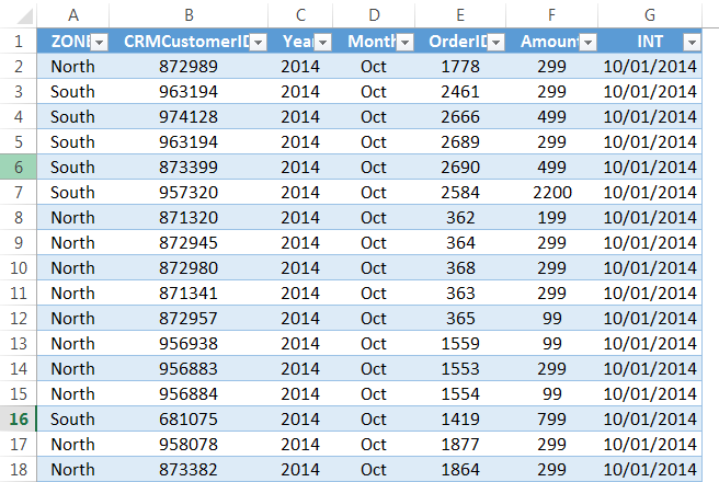
- It will import the data from the selected or connected workbook.

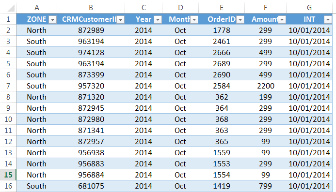
Like this, we can connect to the other workbook and import the data.
#2 – Import Data from MS Access to Excel
MS Access is the main platform to store the data safely. We can import the data directly from the MS Access File itself whenever the data is required.
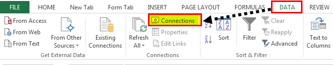
Step 1: Go to the “DATA” ribbon in excelThe ribbon is an element of the UI (User Interface) which is seen as a strip that consists of buttons or tabs; it is available at the top of the excel sheet. This option was first introduced in the Microsoft Excel 2007.read more and select “From Access.“
Step 2: Now, it will ask us to locate the desired file. Select the desired file path. Then, click on “Open.”
Step 3: Now, it will ask us to select the desired destination cell where we want to import the data. Then, click on “OK.”
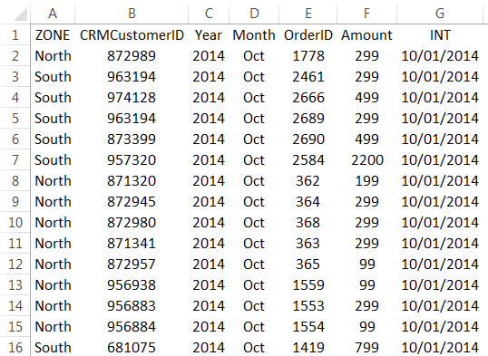
Step 4: It will import the data from access to the A1 cell in Excel.
#3 – Import Data from Text File to Excel
In almost all the corporations, whenever we ask for the data from the IT team, they will write a query and get the file in TEXT format. But unfortunately, TEXT file data is not the ready format to use in Excel; we need to make some modifications to work on it.
Step 1: Go to the “DATA” tab and click on “From Text.”

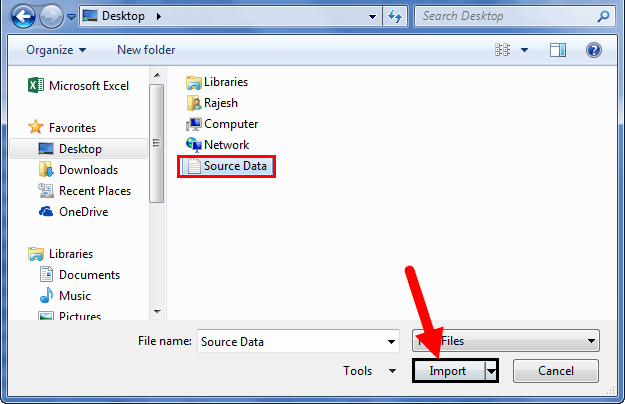
Step 2: Now, it will ask us to choose the file location on the computer or laptop. Select the targeted file, then click on “Import.”
Step 3: It will open up a “Text Import Wizard.”
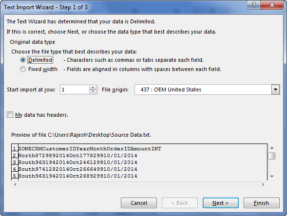
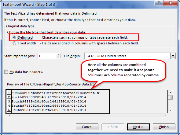
Step 4: By selecting the “Delimited,” click on “Next.”
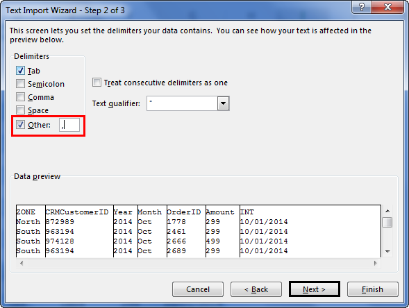
Step 5: In the next window, select the other and mention comma (,) because, in the text file, each column is separated by a comma (,). Then click on “Next.”
Step 6: In the next window, click on “Finish.”
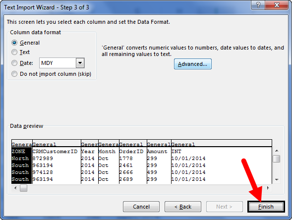
Step 7: Now, it will ask us to select the desired destination cell where we want to import the data. Select the cell and click on “OK.”
Step 8: It will import the data from the text file to the A1 cell in Excel.
Things to Remember
- If there are many tables, we must specify which table data we need to import.
- If we want the data in the current worksheet, we need to select the desired cell. Else, if we need data in a new worksheet, we must choose the new worksheet as the option.
- We need to separate the column in the TEXT file by identifying the common column separators.
Recommended Articles
This article is a guide to Import Data in Excel. Here, we discuss how to import data from 1) Excel Workbook, 2) MS Access, 3) Text File, practical examples, and a downloadable Excel template. You may learn more about Excel from the following articles: –
- KPI Dashboard in Excel
- Insert Image in Excel Cell
- How to Insert New Worksheet In Excel?
- Create a Dashboard in Excel
- Page Numbers in Excel