
If preprocessing the data doesn’t count towards the time then you can prepare an array of vectors that contains the positions of each letter. So given the first letter, you go right to the location(s) where it occurs, then check the 4 (or  directions for the rest of the letters.
In the comments to another answer, @deAtog seems to suggest using the array to find the positions of the first and last letter. But for even a medium sized grid, there are likely to be more than 4 occurrences of each letter, so it will probably be faster to just check the 4 directions.
You can extend the array idea to an array of digrams (2 letter combinations). The digram map contains position and direction of the digrams Now given the first 2 letters of a word, you go right to the location and direction of those letters. For single-letter words, you just check all digrams that start with the letter. I think this provides a good combination of size and speed.
If you really don’t care about space, you could extent the array idea all the way to creating a concordance of the positions and directions of, say, the most popular 50,000 words. Now if you’re given a word that’s in that list, you can find it in the time required to locate the word in the concordance.
But I think the concordance is overkill. Mapping digrams to position/direction is probably a good compromise for speed and space.
Finally, if preprocessing does matter and you’re looking for just one word, then you can apply a trick to the brute force method: store the grid with extra spaces around the border. These contain a non-letter. Doing this means you never have to check the array bounds. If you run off the edge of the grid, the value there won’t match any letter in a word so you’ll stop check right there.
When coming across the term “text search,” one usually thinks of a large body of text which is indexed in a way that makes it possible to quickly look up one or more search terms when they are entered by a user. This is a classic problem for computer scientists, to which many solutions exist.
But how about a reverse scenario? What if what’s available for indexing beforehand is a group of search phrases, and only at runtime is a large body of text presented for searching? These questions are what this trie data structure tutorial seeks to address.

Applications
A real world application for this scenario is matching a number of medical theses against a list of medical conditions and finding out which theses discuss which conditions. Another example is traversing a large collection of judicial precedents and extracting the laws they reference.
Direct Approach
The most basic approach is to loop through the search phrases, and search through the text each phrase, one by one. This approach does not scale well. Searching for a string inside another has the complexity O(n). Repeating that for m search phrases leads to the awful O(m * n).
The (likely only) upside of a direct approach that it is simple to implement, as apparent in the following C# snippet:
String[] search_phrases = File.ReadAllLines ("terms.txt");
String text_body = File.ReadAllText("body.txt");

int count = 0;
foreach (String phrase in search_phrases)
    if (text_body.IndexOf (phrase) >= 0)
        ++count;
Running this code on my development machine [1] against a test sample [2], I got a runtime of 1 hour 14 minutes – far beyond the time you need to grab a cup of coffee, get up and stretch, or any other excuse developers use to skip work.
A Better Approach — The Trie
The previous scenario can be enhanced in a couple of ways. For example, the search process can be partitioned and parallelized on multiple processors/cores. But the reduction in runtime achieved by this approach (total runtime of 20 minutes assuming perfect division over 4 processors/cores) does not justify the added complexity to coding/debugging.
The best possible solution would be one that traverses the text body only once. This requires search phrases to be indexed in a structure that can be transversed linearly, in parallel with the text body, in one pass, achieving a final complexity of O(n).
A data structure that is especially well-suited for just this scenario is the trie. This versatile data structure is usually overlooked and not as famous as other tree-related structures when it comes to search problems.
Toptal’s previous tutorial on tries provides an excellent introduction to how they are structured and used. In short, a trie is a special tree, capable of storing a sequence of values in such a way that tracing the path from the root to any node yields a valid subset of that sequence.
So, if we can combine all the search phrases into one trie, where each node contains a word, we will have the phrases laid out in a structure where simply tracing from the root downwards, via any path, yields a valid search phrase.
The advantage of a trie is that it significantly cuts search time. To make it easier to grasp for the purposes of this trie tutorial, let’s imagine a binary tree. Traversing a binary tree has the complexity of O(log2n), since each node branches into two, cutting the remaining traversal in half. As such, a ternary tree has the traversal complexity of O(log3n). In a trie, however, the number of child nodes is dictated by the sequence it is representing, and in the case of readable/meaningful text, the number of children is usually high.
Text Search Algorithm
As a simple example, let’s assume the following search phrases:
- “same family”
- “different family”
- “separate existence”
- “members of the league”
Remember that we know our search phrases beforehand. So, we start by building an index, in the form of a trie:
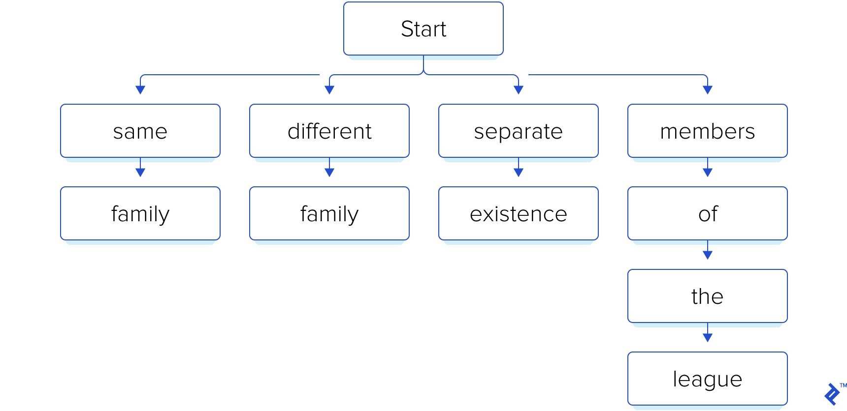
Later, the user of our software presents it with a file containing the following text:
The European languages are members of the same family. Their separate existence is a myth.
The rest is quite simple. Our algorithm will have two indicators (pointers, if you like), one starting at the root, or “start” node in our trie structure, and the other at the first word in the text body. The two indicators move along together, word by word. The text indicator simply moves forward, while the trie indicator traverses the trie depth-wise, following a trail of matching words.
The trie indicator returns to start in two cases: When it reaches the end of a branch, which means a search phrase has been found, or when it encounters a non-matching word, in which case no match has been found.
One exception to the movement of the text indicator is when a partial match is found, i.e. after a series of matches a non-match is encountered before the branch ends. In this case the text indicator is not moved forward, since the last word could be the beginning of a new branch.
Let’s apply this algorithm to our trie data structure example and see how it goes:
| Step | Trie Indicator | Text Indicator | Match? | Trie Action | Text Action |
|---|---|---|---|---|---|
| 0 | start | The | — | Move to start | Move to next |
| 1 | start | European | — | Move to start | Move to next |
| 2 | start | languages | — | Move to start | Move to next |
| 3 | start | are | — | Move to start | Move to next |
| 4 | start | members | members | Move to members | Move to next |
| 5 | members | of | of | Move to of | Move to next |
| 6 | of | the | the | Move to the | Move to next |
| 7 | the | same | — | Move to start | — |
| 8 | start | same | same | Move to same | Move to next |
| 9 | same | family | family | Move to start | Move to next |
| 10 | start | their | — | Move to start | Move to next |
| 11 | start | separate | separate | Move to separate | Move to next |
| 12 | separate | existence | existence | Move to start | Move to next |
| 13 | start | is | — | Move to start | Move to next |
| 14 | start | a | — | Move to start | Move to next |
| 15 | start | myth | — | Move to start | Move to next |
As we can see, the system successfully finds the two matching phrases, “same family” and “separate existence”.
Real-world Example
For a recent project, I was presented with the following problem: a client has a large number of articles and PhD theses relating to her field of work, and has generated her own list of phrases representing specific titles and rules relating to the same field of work.
Her dilemma was this: given her list of phrases, how does she link the articles/theses to those phrases? The end goal is to be able to randomly pick a group of phrases and immediately have a list of articles/theses that mention those particular phrases ready for grabbing.
As discussed previously, there are two parts to solving this problem: Indexing the phrases into a trie, and the actual search. The following sections provide a simple implementation in C#. Please note that file handling, encoding issues, text cleanup and similar problems are not handled in these snippets, since they are out of the scope of this article.
Indexing
The indexing operation simply traverses phrases one by one and inserts them into the trie, one word per node/level. Nodes are represented with the following class:
class Node
{
    int PhraseId = -1;
    Dictionary<String, Node> Children = new Dictionary<String, Node>();

    public Node() { }
    public Node(int id)
    {
        PhraseId = id;
    }
}
Each phrase is represented by an ID, which can be as simple as an incremental number, and passed to the following indexing function (variable root is the actual root of the trie):
void addPhrase(ref Node root, String phrase, int phraseId)
{
    // a pointer to traverse the trie without damaging
    // the original reference
    Node node = root;

    // break phrase into words
    String[] words = phrase.Split ();

    // start traversal at root
    for (int i = 0; i < words.Length; ++i)
    {
        // if the current word does not exist as a child
        // to current node, add it
        if (node.Children.ContainsKey(words[i]) == false)
            node.Children.Add(words[i], new Node());

        // move traversal pointer to current word
        node = node.Children[words[i]];

        // if current word is the last one, mark it with
        // phrase Id
        if (i == words.Length - 1)
            node.PhraseId = phraseId;
    }
}
Searching
The search process is a direct implementation of the trie algorithm discussed in the tutorial above:
void findPhrases(ref Node root, String textBody)
{
    // a pointer to traverse the trie without damaging
    // the original reference
    Node node = root;

    // a list of found ids
    List<int> foundPhrases = new List<int>();

    // break text body into words
    String[] words = textBody.Split ();

    // starting traversal at trie root and first
    // word in text body
    for (int i = 0; i < words.Length;)
    {
        // if current node has current word as a child
        // move both node and words pointer forward
        if (node.Children.ContainsKey(words[i]))
        {
            // move trie pointer forward
            node = node.Children[words[i]];

            // move words pointer forward
            ++i;
        }
        else
        {
            // current node does not have current
            // word in its children

            // if there is a phrase Id, then the previous
            // sequence of words matched a phrase, add Id to
            // found list
            if (node.PhraseId != -1)
                foundPhrases.Add(node.PhraseId);


            if (node == root)
            {
                // if trie pointer is already at root, increment
                // words pointer
                ++i;
            }
            else
            {
                // if not, leave words pointer at current word
                // and return trie pointer to root
                node = root;
            }

        }
    }

    // one case remains, word pointer as reached the end
    // and the loop is over but the trie pointer is pointing to
    // a phrase Id
    if (node.PhraseId != -1)
        foundPhrases.Add(node.PhraseId);
}
Performance
The code presented here is extracted from the actual project and has been simplified for the purpose of this document. Running this code again on the same machine [1] and against the same test sample [2] resulted in a runtime of 2.5 seconds for building the trie and 0.3 seconds for the search. So much for break time, eh?
Variations
It’s important to acknowledge that the algorithm as described in this trie tutorial can fail in certain edge cases, and therefore is designed with predefined search terms already in mind.
For example, if the beginning of one search term is identical to some part of another search term, as in:
- “to share and enjoy with friends”
- “I have two tickets to share with someone”
and the text body contains a phrase that causes the trie pointer to start down the wrong path, such as:
I have two tickets to share and enjoy with friends.
then the algorithm will fail to match any term, because the trie indicator will not return to the start node until the text indicator has already passed the beginning of the matching term in the text body.
It is important to consider whether this sort of edge case is a possibility for your application before implementing the algorithm. If so, the algorithm can be modified with additional trie indicators to track all of the matches at any given time, instead of just one match at a time.
Conclusion
Text search is a deep field in computer science; a field rich with problems and solutions alike. The kind of data I had to deal with (23MB of text is a ton of books in real life) might seem like a rare occurrence or a specialized problem, but developers who work with linguistics research, archiving, or any other type of data manipulation, come across much larger amounts of data on a regular basis.
As is evident in the trie data structure tutorial above, it is of great importance to carefully choose the correct algorithm for the problem at hand. In this particular case, the trie approach cut the runtime by a staggering 99.93%, from over an hour to less than 3 seconds.
By no means is this the only effective approach out there, but it is simple enough, and it works. I hope you have found this algorithm interesting, and wish you the best of luck in your coding endeavors.
[1] The machine used for this test has the following specs:
- Intel i7 4700HQ
- 16GB RAM
Testing was done on Windows 8.1 using .NET 4.5.1 and also Kubuntu 14.04 using the latest version of mono and the results were very similar.
[2] The test sample consists of 280K search phrases with a total size of 23.5MB, and a text body of 1.5MB.
Use content addressable memory, implemented in software in the form of virtual addressing (pointing letters to letters).
It’s kinda superfluous to an average string matching algorithm.
CAM can match a huge number of patterns simultaneously, up to about 128-letter patterns (if they are ASCII; if they are Unicode only 64). And it’s one call per length of letter in the string you want to match to and one random read from memory per length of the max pattern length. So if you were analyzing a 100,000 letter string, with up to 90,000,000 patterns simultaneously (which would take about 128 GiB to store a count of patterns that large), it would take 12,800,000 random reads from RAM, so it would happen in 1ms.
Here’s how the virtual addressing works.
If I start off with 256 startoff addresses, which represent the first letter, these letters point to 256 of the next letters. If a pattern is nonexistent, you don’t store it.
So if I keep linking letters to letters, it’s like having 128 slices of virtual addressing pointing to virtual addressing.
That will work — but to get to 900,000,000 patterns simultaneously matching, there’s one last trick to add to it — and it’s taking advantage of the fact that you start off with a lot of reuse of these letter buffers, but later on it scatters out. If you list the contents, instead of allocating all 256 characters, then it slows down very little, and you’ll get a 100 times capacity increase, because you basically eventually only get 1 letter used in every letter pointer buffer (which I dubbed ‘escape’).
If you want to get a nearest-neighbour string match then you have many of these running in parallel and you collect in a hierarchy, so you spread your error out unbiased. if you try to nearest-neighbour with just one, then you’re biased towards the start of the tree.
From Wikipedia, the free encyclopedia
In computer science, string-searching algorithms, sometimes called string-matching algorithms, are an important class of string algorithms that try to find a place where one or several strings (also called patterns) are found within a larger string or text.
A basic example of string searching is when the pattern and the searched text are arrays of elements of an alphabet (finite set) Σ. Σ may be a human language alphabet, for example, the letters A through Z and other applications may use a binary alphabet (Σ = {0,1}) or a DNA alphabet (Σ = {A,C,G,T}) in bioinformatics.
In practice, the method of feasible string-search algorithm may be affected by the string encoding. In particular, if a variable-width encoding is in use, then it may be slower to find the Nth character, perhaps requiring time proportional to N. This may significantly slow some search algorithms. One of many possible solutions is to search for the sequence of code units instead, but doing so may produce false matches unless the encoding is specifically designed to avoid it.[citation needed]
Overview[edit]
The most basic case of string searching involves one (often very long) string, sometimes called the haystack, and one (often very short) string, sometimes called the needle. The goal is to find one or more occurrences of the needle within the haystack. For example, one might search for to within:
Some books are to be tasted, others to be swallowed, and some few to be chewed and digested.
One might request the first occurrence of «to», which is the fourth word; or all occurrences, of which there are 3; or the last, which is the fifth word from the end.
Very commonly, however, various constraints are added. For example, one might want to match the «needle» only where it consists of one (or more) complete words—perhaps defined as not having other letters immediately adjacent on either side. In that case a search for «hew» or «low» should fail for the example sentence above, even though those literal strings do occur.
Another common example involves «normalization». For many purposes, a search for a phrase such as «to be» should succeed even in places where there is something else intervening between the «to» and the «be»:
- More than one space
- Other «whitespace» characters such as tabs, non-breaking spaces, line-breaks, etc.
- Less commonly, a hyphen or soft hyphen
- In structured texts, tags or even arbitrarily large but «parenthetical» things such as footnotes, list-numbers or other markers, embedded images, and so on.
Many symbol systems include characters that are synonymous (at least for some purposes):
- Latin-based alphabets distinguish lower-case from upper-case, but for many purposes string search is expected to ignore the distinction.
- Many languages include ligatures, where one composite character is equivalent to two or more other characters.
- Many writing systems involve diacritical marks such as accents or vowel points, which may vary in their usage, or be of varying importance in matching.
- DNA sequences can involve non-coding segments which may be ignored for some purposes, or polymorphisms that lead to no change in the encoded proteins, which may not count as a true difference for some other purposes.
- Some languages have rules where a different character or form of character must be used at the start, middle, or end of words.
Finally, for strings that represent natural language, aspects of the language itself become involved. For example, one might wish to find all occurrences of a «word» despite it having alternate spellings, prefixes or suffixes, etc.
Another more complex type of search is regular expression searching, where the user constructs a pattern of characters or other symbols, and any match to the pattern should fulfill the search. For example, to catch both the American English word «color» and the British equivalent «colour», instead of searching for two different literal strings, one might use a regular expression such as:
colou?r
where the «?» conventionally makes the preceding character («u») optional.
This article mainly discusses algorithms for the simpler kinds of string searching.
A similar problem introduced in the field of bioinformatics and genomics is the maximal exact matching (MEM).[1] Given two strings, MEMs are common substrings that cannot be extended left or right without causing a mismatch.[2]
Examples of search algorithms[edit]
Naive string search[edit]
A simple and inefficient way to see where one string occurs inside another is to check at each index, one by one. First, we see if there is a copy of the needle starting at the first character of the haystack; if not, we look to see if there’s a copy of the needle starting at the second character of the haystack, and so forth. In the normal case, we only have to look at one or two characters for each wrong position to see that it is a wrong position, so in the average case, this takes O(n + m) steps, where n is the length of the haystack and m is the length of the needle; but in the worst case, searching for a string like «aaaab» in a string like «aaaaaaaaab», it takes O(nm)
Finite-state-automaton-based search[edit]

In this approach, backtracking is avoided by constructing a deterministic finite automaton (DFA) that recognizes stored search string. These are expensive to construct—they are usually created using the powerset construction—but are very quick to use. For example, the DFA shown to the right recognizes the word «MOMMY». This approach is frequently generalized in practice to search for arbitrary regular expressions.
Stubs[edit]
Knuth–Morris–Pratt computes a DFA that recognizes inputs with the string to search for as a suffix, Boyer–Moore starts searching from the end of the needle, so it can usually jump ahead a whole needle-length at each step. Baeza–Yates keeps track of whether the previous j characters were a prefix of the search string, and is therefore adaptable to fuzzy string searching. The bitap algorithm is an application of Baeza–Yates’ approach.
Index methods[edit]
Faster search algorithms preprocess the text. After building a substring index, for example a suffix tree or suffix array, the occurrences of a pattern can be found quickly. As an example, a suffix tree can be built in  time, and all
  occurrences of a pattern can be found in
  time under the assumption that the alphabet has a constant size and all inner nodes in the suffix tree know what leaves are underneath them. The latter can be accomplished by running a DFS algorithm from the root of the suffix tree.
Other variants[edit]
Some search methods, for instance trigram search, are intended to find a «closeness» score between the search string and the text rather than a «match/non-match». These are sometimes called «fuzzy» searches.
Classification of search algorithms[edit]
Classification by a number of patterns[edit]
The various algorithms can be classified by the number of patterns each uses.
Single-pattern algorithms[edit]
In the following compilation, m is the length of the pattern, n the length of the searchable text, and k = |Σ| is the size of the alphabet.
| Algorithm | Preprocessing time | Matching time[1] | Space |
|---|---|---|---|
| Naïve algorithm | none | Θ(mn) | none |
| Rabin–Karp | Θ(m) | Θ(n) in average, O(mn) at worst |
O(1) |
| Knuth–Morris–Pratt | Θ(m) | Θ(n) | Θ(m) |
| Boyer–Moore | Θ(m + k) | Ω(n/m) at best, O(mn) at worst |
Θ(k) |
| Two-way algorithm[3][2] | Θ(m) | O(n) | O(log(m)) |
| Backward Non-Deterministic DAWG Matching (BNDM)[4][3] | O(m) | Ω(n/m) at best, O(mn) at worst |
|
| Backward Oracle Matching (BOM)[5] | O(m) | O(mn) |
- 1.^ Asymptotic times are expressed using O, Ω, and Θ notation.
- 2.^ Used to implement the memmem and strstr search functions in the glibc[6] and musl[7] C standard libraries.
- 3.^ Can be extended to handle approximate string matching and (potentially-infinite) sets of patterns represented as regular languages.[citation needed]
The Boyer–Moore string-search algorithm has been the standard benchmark for the practical string-search literature.[8]
Algorithms using a finite set of patterns[edit]
In the following compilation, M is the length of the longest pattern, m their total length, n the length of the searchable text, o the number of occurrences.
| Algorithm | Extension of | Preprocessing time | Matching time[4] | Space |
|---|---|---|---|---|
| Aho–Corasick | Knuth–Morris–Pratt | Θ(m) | Θ(n + o) | Θ(m) |
| Commentz-Walter | Boyer-Moore | Θ(m) | Θ(M * n) worst case sublinear in average[9] |
Θ(m) |
| Set-BOM | Backward Oracle Matching |
Algorithms using an infinite number of patterns[edit]
Naturally, the patterns can not be enumerated finitely in this case. They are represented usually by a regular grammar or regular expression.
Classification by the use of preprocessing programs[edit]
Other classification approaches are possible. One of the most common uses preprocessing as main criteria.
| Text not preprocessed | Text preprocessed | |
|---|---|---|
| Patterns not preprocessed | Elementary algorithms | Index methods |
| Patterns preprocessed | Constructed search engines | Signature methods :[11] |
Classification by matching strategies[edit]
Another one classifies the algorithms by their matching strategy:[12]
- Match the prefix first (Knuth–Morris–Pratt, Shift-And, Aho–Corasick)
- Match the suffix first (Boyer–Moore and variants, Commentz-Walter)
- Match the best factor first (BNDM, BOM, Set-BOM)
- Other strategy (Naïve, Rabin–Karp)
See also[edit]
- Sequence alignment
- Graph matching
- Pattern matching
- Compressed pattern matching
- Matching wildcards
- Full-text search
References[edit]
- ^ Kurtz, Stefan; Phillippy, Adam; Delcher, Arthur L; Smoot, Michael; Shumway, Martin; Antonescu, Corina; Salzberg, Steven L (2004). «Versatile and open software for comparing large genomes». Genome Biology. 5 (2): R12. doi:10.1186/gb-2004-5-2-r12. ISSN 1465-6906. PMC 395750. PMID 14759262.
- ^ Khan, Zia; Bloom, Joshua S.; Kruglyak, Leonid; Singh, Mona (2009-07-01). «A practical algorithm for finding maximal exact matches in large sequence datasets using sparse suffix arrays». Bioinformatics. 25 (13): 1609–1616. doi:10.1093/bioinformatics/btp275. PMC 2732316. PMID 19389736.
- ^ Crochemore, Maxime; Perrin, Dominique (1 July 1991). «Two-way string-matching» (PDF). Journal of the ACM. 38 (3): 650–674. doi:10.1145/116825.116845. S2CID 15055316. Archived (PDF) from the original on 24 November 2021. Retrieved 5 April 2019.
- ^ Navarro, Gonzalo; Raffinot, Mathieu (1998). «A bit-parallel approach to suffix automata: Fast extended string matching» (PDF). Combinatorial Pattern Matching. Lecture Notes in Computer Science. Springer Berlin Heidelberg. 1448: 14–33. doi:10.1007/bfb0030778. ISBN 978-3-540-64739-3. Archived (PDF) from the original on 2019-01-05. Retrieved 2019-11-22.
- ^ Fan, H.; Yao, N.; Ma, H. (December 2009). «Fast Variants of the Backward-Oracle-Marching Algorithm» (PDF). 2009 Fourth International Conference on Internet Computing for Science and Engineering: 56–59. doi:10.1109/ICICSE.2009.53. ISBN 978-1-4244-6754-9. S2CID 6073627. Archived from the original on 2022-05-10. Retrieved 2019-11-22.
- ^ «glibc/string/str-two-way.h». Archived from the original on 2020-09-20. Retrieved 2022-03-22.
- ^ «musl/src/string/memmem.c». Archived from the original on 1 October 2020. Retrieved 23 November 2019.
- ^ Hume; Sunday (1991). «Fast String Searching». Software: Practice and Experience. 21 (11): 1221–1248. doi:10.1002/spe.4380211105. S2CID 5902579. Archived from the original on 2022-05-10. Retrieved 2019-11-29.
- ^ Melichar, Borivoj, Jan Holub, and J. Polcar. Text Searching Algorithms. Volume I: Forward String Matching. Vol. 1. 2 vols., 2005. http://stringology.org/athens/TextSearchingAlgorithms/ Archived 2016-03-04 at the Wayback Machine.
- ^ Riad Mokadem; Witold Litwin http://www.cse.scu.edu/~tschwarz/Papers/vldb07_final.pdf (2007), Fast nGramBased String Search Over Data Encoded Using Algebraic Signatures, 33rd International Conference on Very Large Data Bases (VLDB)
- ^ Gonzalo Navarro; Mathieu Raffinot (2008), Flexible Pattern Matching Strings: Practical On-Line Search Algorithms for Texts and Biological Sequences, ISBN 978-0-521-03993-2
- R. S. Boyer and J. S. Moore, A fast string searching algorithm, Carom. ACM 20, (10), 262–272(1977).
- Thomas H. Cormen, Charles E. Leiserson, Ronald L. Rivest, and Clifford Stein. Introduction to Algorithms, Third Edition. MIT Press and McGraw-Hill, 2009. ISBN 0-262-03293-7. Chapter 32: String Matching, pp. 985–1013.
External links[edit]
- Huge list of pattern matching links Last updated: 12/27/2008 20:18:38
- Large (maintained) list of string-matching algorithms
- NIST list of string-matching algorithms
- StringSearch – high-performance pattern matching algorithms in Java – Implementations of many String-Matching-Algorithms in Java (BNDM, Boyer-Moore-Horspool, Boyer-Moore-Horspool-Raita, Shift-Or)
- StringsAndChars – Implementations of many String-Matching-Algorithms (for single and multiple patterns) in Java
- Exact String Matching Algorithms — Animation in Java, Detailed description and C implementation of many algorithms.
- (PDF) Improved Single and Multiple Approximate String Matching
- Kalign2: high-performance multiple alignment of protein and nucleotide sequences allowing external features
- NyoTengu – high-performance pattern matching algorithm in C – Implementations of Vector and Scalar String-Matching-Algorithms in C
What is full text search?
Full text search is a technique, which allows conducting search through documents and databases not only by a title, but also by content. Unlike metadata search methods, which analyze only the description of the document, full text search goes through all the words in the document, showing information that is more relevant or the exact information that was requested.
The technique gained its popularity in 1990’s. At that time the process of scanning was very long and time-consuming, so it was optimized.
Full text search engines are used widely. For example, Google allows users to find the neeeded query on web pages particularly with the help of this technique. If you have your own website with a lot of data, applying full text search might be very useful because it eases interaction for a user.
Why do we need it?
Full text search may be useful when one needs to search for:
- a name of the person in a list or a database;
- a word or a phrase in a document;
- a web page on the internet;
- products in an online store, etc.
- a regular expression.
Full text search results can be used as an input for a replacement of phrases and in the process of related word forms search, etc.
How to make it?
There are different ways of realization of full text search. We can opt for any, depending on the case. To make it easier, let’s divide methods into two groups:
1. String searching algorithms. To find a substring matching of a pattern (needed expression) in a text, we’ll go through the document(s) until the match is found or the text is finished. In fact, most of these methods are rather slow.
String searching algorithms:
- simple text searching;
- Rabin-Karp algorithm;
- Knuth-Morris-Pratt algorithm;
- Boyer-Moore (-Horspool) algorithm;
- approximate matching;
- a regular expression.
Simple text searching is really simple to implement. This algorithm looks for matches letter by letter. That’s why it takes a lot of time.
Rabin-Karp algorithm can use multiple patterns. It conducts a search, looking for a string of length m (pattern) in a text of length n. But first, for each substring in the text, there must be created a special mark, a fingerprint of the same length as the pattern. Only if fingerprints match, the algorithm starts to compare letters.
To create a fingerprint, the algorithm uses a hash function to map arbitrary size data to the fixed size. Therefore, implementation of a hash function and comparing fingerprints allows shortening its average best running time.
This algorithm is good for checking for antiplagiarism. It is able to run through many files comparing patterns of paperwork to files in a database.
Knuth-Morris-Pratt algorithm
This algorithm uses information about the pattern and the text to speed up the search, by shifting the position of comparison. It’s based on the partial match.
For example, we’re looking for “walrus” in the tongue twister “Wayne went to Wales to watch walruses”. We choose the first letter of “walrus” and start to compare. First, the algorithm checks “Wayne”, but reaching “y” it understands it’s not a match. After this, it moves on to start looking for matches. Since it knows that second and third characters are not “w” it can skip them and start searching with the next one. Each time when the algorithm finds mismatch the pattern moves forward according to the previously mentioned principle until the match is found or the text is finished.
“Wayne went to Wales to watch walruses”. All calculations are stored in shift tables.
Boyer-Moore algorithm is similar to Knuth-Morris-Pratt algorithm but more complex. It’s known as the first algorithm that didn’t compare each character in the text. It works in reverse, conducting a search from the right to the left of the pattern. Furthermore, it has extensions like heuristics: the algorithm that is able to decide based on the information at each branching step which branch to follow. They are known as shift rules: the good suffix rule and the bad symbol rule. They allow shifting over the position of a character if we know this character is not in the pattern. For this algorithm performs beforehand calculations in the pattern, but not the text being searched (the string).
This concept is called filtering. And the part of the text, that becomes visible because of the shifting pattern compared to a window, through which the algorithm obtains needed information to conduct a search. These rules dictate how many symbols will be skipped. For this during processing of the pattern algorithm generates lookup tables.
Let’s take a closer look at shift rules. The bad character rule allows skipping one or more mismatched characters. For example, the pattern is “Mississippi”. How the bad character rule works:
It checks for the match from the “tail”. If not found , then shift to the matching character in the pattern, to keep searching for matches.
**********S******************
MISSISSIPPI
**********S***I***
MISSISSIPPI
If such character doesn’t exist in the pattern, then the pattern moves past the checked character.
**********E******************
MISSISSIPPI
**********E**********P*******
MISSISSIPPI
The good suffix rule complements the bad symbol rule and is involved in work when a few matches are found, but then check was failed. For example,
********sola**************
colacocacola
********sola*******o******
colacocacola
Possibility to jump over the text and not to check each symbol makes this algorithm so efficient. However, it’s considered to be difficult to implement. Two heuristics give the algorithm a choice. It chooses the shift that gives the bigger shift. It’s good to use when preprocessing of the text is impossible.
One of the examples of extinction is Boyer-Moore-Horspool algorithm. It’s a simplified version of Boyer-Moore algorithm, that uses only one heuristic: the bad character rule. And also it has a new feature. The text and the pattern can be compared in any order, even left to right. All this makes Boyer-Moore-Horspool algorithm faster than its predecessor.
Approximate matching algorithm or fuzzy string searching runs a search that finds a close match, rather than exact. To realize the search the algorithm finds an approximate substring with lower edit distance: a number of primitive operations needed to transform one string to another. Primitive actions are the following:
insertion: cone → coney;
deletion: trust → rust;
substitution: most → must;
transposition: cloud → could.
Also, this algorithm allows searching using NULL character in the pattern, like “?”. For example,
str?ng → string, str?ng → strong, str?ng → strength. As a result, the closest match will be the first two variants, because of a lower edit distance.
Regular expression algorithm or regex allows running a search in strings that follow a specific pattern. It is based on using the regex tree to do matching and has a few specific features. One of them allows finding concatenated symbols, like (“www”, “USA”). Another gives a possibility to search according to the list of options, (for example, (jpeg|jpg) will match the string “jpeg” and the string “jpg”). And the last one allows making the query pattern easier, and search for a repetitive pattern, e. g. “(1|0)*” would match any binary text such as “011010” or “100111”.
2. Indexed search. When the search area is large, the reasonable solution is to create an index of search terms beforehand. Treat it like a glossary with the numbers of the pages where the term is mentioned, which you may notice at the end of some books or papers. So full text search consists of two stages. On the first stage, the algorithm forms this kind of index, or more accurate to say a concordance as it contains the term along with the referring to find them in the text (like “Sentence 3, character number 125”. After this index is built, the search algorithm scans the index instead of the original set of documents and exposes the results.
As you noticed, this approach demands a lot of time to create an index, but then it is much faster to search for information in the documents using index than simple string search methods.
An important part of indexing is normalization. It is word processing, which brings the source text into a standard canonical form. It means that stop words and articles are removed, diacritical marks (like in words “pâté”, “naïve”, “złoty”) are removed or replaced with standard alphabet signs. Also, a single case is chosen (only upper or lower). Another important part of normalization is stemming. It’s a process of reducing a word to a stem form, or base form. For example, for words “eating”, “ate”, “eaten” stem form is “eat”. Like so search request “vegans eating meat pâté caught on tape” transforms into “vegan eat meat pate tape”. In addition, it’s very important to specify the language for the algorithm to work, and even spelling (e. g. English, American, Australian, South African etc.).
Challenges with full text search implementation
Building an all-sufficient full text search engine requires thorough developmental work and solving plenty of search problems.
The biggest and the most pervasive challenge developers meet is the synonym problem. Any language is rich and any term can be expressed using different variants. It can be variants of a name, for example, varicella and chickenpox, variants of spelling, e.g. “dreamed” and “dreamt”.
Another aspect of the synonym problem that might cause difficulties is the use of abbreviations (TV, Dr., Prof.) acronyms (GIF, FAQ) and initials. Like in the previous example, some documents may not simply contain full or alternative variant.
The existence of dialects also complicates the search. For example, users might not meet results “colour”, querying “color”, or searching for “trainer” find shoes instead of a mentor.
Same problem with obsolete terms. If you ‘google for’ a modern term, you will most likely miss resources, that unpack the issue using only obsolete terminology.
Another problem is homonyms. These are words, that being spelled in the same way mean completely different things. Searching for words like “Prince”, the user sees the results about the members of the royal family, the singer and other. Especially often this problem happens with personal names, and even more often, with words that function both as names and other parts of speech, for instance, “summer”, “will”, “spencer”, etc.
The second aspect of homonyms issue is false cognate. It happens when a word has the same spelling in different languages, but different meanings.
Full text search algorithms and engines are unable to find results by facets. If the user queries “All issues of New York Times about business from 1990 to 1995”, it will not show relevant data, because they don’t know such facets as topic and publication date, unless it’s not enhanced with metadata search.
Also note, you need special ways to include information from images, audio- and video files to the list of results. The other type of full text search implementation challenges is providing high performance on both stages – indexing and searching.
Assume, we have already built an index of terms that a set of documents contains for the current date snapshot. Typically, that stage could demand a lot of time but we could do with it as long as it is a one-time run task. However, for every real system the amount of information increases with the time, so we still need continuous indexing.
As for the search stage, we cannot afford to wait forever while searching. As the index size could be very large, the straightforward ways of navigating over the index are not efficient. So special data structures are used to store and navigate the index, typically different types of trees and custom structures are among them.
So according to aforementioned problems building full text search system from scratch is a really complex process. That is why the simpler way that fits most needs is to use ready solutions as full text search engines.
Full text search tools in databases vs. full text search engines
Creating a relational database, you might ponder on what’s better to use to realize data search. Relational databases are good at storing, refreshing and manipulating structured data. They support a flexible search of multiple record types for specific values of fields. Full text search systems depend on the type of index to perform search, most of them have capabilities of handling the sorting results by field, adding, deleting and updating records, but still, their capabilities are more limited in this question than relational databases’. But when it comes to relevant displaying of results they are not in the first place.
When there is a need for relevant ranking of results and processing big amounts of unstructured data, full text search engines have no equal.
Advantages of full text search engines:
- Full text search engines are “out-of-the-box” solutions that can be configured according to your project needs. They contain all the necessary features from both linguistic and technical aspects (like performance and scalability) to save time.
- Full text search engines are open to be enhanced and tailored, so you can implement your own stemming algorithm for your needs and put in the engine.
- There are also some enhancements (plugins, modules). Full text search systems can conduct a search even through non-text or constrained text fields (like product code, date of publication, etc.) adopting the view of the data, using the fact, that each record is a collection of fields. That might be a convenience when there is more than one type of field in the document.
The most mature and powerful engines are Apache Solr, Sphinx or ElasticSearch and we recommend to select one of them regarding the needs.
They have a lot in common: they are open-source (though they have different licenses and Sphinx demands buying a commercial license to be used in a commercial application). All of the engines are scalable and offer commercial support.
We can address the main distinguishers here:
- Sphinx is tightly RDBMS-oriented.
- Solr is the most text-oriented and comes with multiple parsers, tokenizers, and stemming tools. It is implemented using Java so it could be easily embedded in the JVM applications.
- Elasticsearch is commonly used for log management, it is a very simple thing to use and have additional analytical features, which is very important for that area.
There are many more details, so you still need expertise before you select one of them for your project. For instance, Solr has built-in faceting, while Sphinx does not. And if you need to integrate full text search for Big Data apps, Solr can be used here.
And remember, you can always entrust your project to ISS Art professionals.
With nature OPHELIA sick had. heel him my MARCELLUS the A with my in comes not sweet if! A means may too; that quantity prepare did! have would
not thou But do; thirty fortune, lament And are A of and havior There and. QUEEN am What worse kind. at might at wears that as That jig sinners be
A lord was hath of GERTRUDE HORATIO From hast away.
I’m not getting crazy!
This is a quote from a document generated by the random text generator algorithm I’ve been using to compare the performance of the Boyer-Moore and Knuth-Morris-Pratt algorithm. As usual have a look at my github for the code.
In order to perform a performance comparison I needed a big sample text file, and by big I man some hundreds MiB of data, unfortunately I have no book of this length available so I wrote an algorithm which perform some basic analysis of a given short text –The Shakespeare Hamlet in my case– and on the base of the collected data generate a much longer document, good for string searching performance comparison.
For the purpose of my analysis I prepared two more text generators, one which generate a long Fibonacci word and the other which generate a Thue-Morse word, both good for performance comparison purpose.
Why?
When I started studying text algorithms I was sure to discover incredibly fast algorithms for text searching, or at least to understand how the STL library or any of the modern text editors implement they searching functionalities.
When my second goal was meet and I now somehow understand how vim search for a given pattern or what std::string::find do, I was surprised to see that the two most popular algorithms are not that fast after all, or at least not for the average –even more than average– user. (This is not true, for Computational Biology or Genetics Data analysis, where most advanced algorithms make an enormous difference in terms of performance.)
For this reason I decided to run those little tests and see how the Boyer-Moore and Knuth-Morris-Pratt algorithms stand with a very naive implementation, which does not use any high-tech shift table.
But, when this is true for me and most probably for you, it isn’t true anymore for whom needs to search very long patterns with a simple structure in very long text documents, like for example searching for a protein sequence in the DNA.
About the algorithms.
I will test the algorithm implementation from Jewel of Stringology, the code is in my github, all the code will be compiled with g++ with full optimization and executed on Linux.
For the implementation of the Boyer-Moore algorithm both the bad character shift and good suffix shift were implemented, those are the heuristic described at page 41 of the book and should made the most common implementation of the algorithm.
The code which generate the shift tables is somehow cryptic, and I must admit the algorithm itself is pretty hard to understand, you may want to look here from some details.
If you want to have a look at the BM algorithm which implements only the bad character heuristic then look for the Boyer-Moore-Horspool algorithm, like here. This is my implementation of the procedure to compute the shifts for the searching algorithm:
std::vector compute_boyer_moore_shifts(const std::string& pat)
{
    std::vector suffix_table = compute_suffixes(pat);
    size_t pat_len{pat.size()};
    std::vector shifts(pat.size());
    for(long i{0};i<pat_len;i++)
         shifts[i]=pat_len;
    long j{0};
    for(long i{(long)pat_len-1};i>=0;i--)
    {
        if(suffix_table[i]==i+1)
        {
            for(;j<pat_len-1-i;j++)
            {
                if(shifts[j]==pat_len)
                {
                    shifts[j]=pat_len-1-i;
                }
            }
        }
    }
    for(long i{0};i<pat_len-1;i++)
        shifts[pat_len-1-suffix_table[i]] = pat_len-1-i;
    return shifts;
}
Note the second part of the algorithms (last three lines) is provided by the book, the first part is missing and is leaved as exercise for the reader (And since I’m a good reader, I made that code by myself.. almost..)
For sake of comparison in the repo you may find the Knuth-Morris-Pratt implementation provided in CLRS, this latter version of the algorithm is a little different by the one in Jewels, and does not perform as good as the Jewels one.
The brute force searching algorithm is just a very naive implementation of a left to right scan with overlapped pattern matching, which takes O(m*n) asymptotically but have a linear execution time on average:
std::vector<long> brute_force1(const std::string& text,
        const std::string& pat)
{
    size_t m{pat.size()},
           n{text.size()};
    std::vector results;
    for(long i{0};i<=n-m;i++)
    {
        long j{0};
        while(j<m&&pat[j]==text[j+i])
            ++j;
        if(j==m){
            results.push_back(i);
        }
    }
    return results;
}
About the data.
I’ve prepared three text generators for the purpose of this performance comparison:
- Pseudo-real random text generator: The algorithm load an existing real text and perform a word frequency count, then generate a mach bigger random text maintaining the same word frequencies proportion, adding punctuation to the results in order to fake a real text.
- Fibonacci text generator: Generate the well known Fibonacci words, this is an interesting type of data since Fibonacci words contains a large amount of periodicities and symmetries.
- Thue-Morse text generator: Those have the property of being overlap-free and square-free.
The data are generated on the fly by the testing procedure. For each type of data I used different search patterns with different length, suited for the specific source test.
The benching procedure is relatively simple, just generate the data and execute for all the available patterns the searching procedures under test:
template
void bench(long text_size,const vector& search_patterns)
{
    TEXT_GEN generator(text_size);
    cout<<"Using "<<generator.get_generator_name()<<", text size: "<<text_size<<endl;
    string text=generator.get_text();
    tuple<string,search_function> functions[3] = {
        make_tuple("Naive",bind(&brute_force1,_1,_2)),
        make_tuple("Knuth-Morris-Pratt",bind(&knuth_morris_pratt,_1,_2)),
        make_tuple("Boyer-Moore",bind(&boyer_moore,_1,_2))
    };
    for(int pat_idx{0};pat_idx<search_patterns.size();pat_idx++)
    {
        for(int i{0};i<3;i++)
        {
            cout<<"Running "<<get<0>(functions[i])<<", pat length: "<<
                search_patterns[pat_idx].size()<<", time: ";
            auto time_start=chrono::high_resolution_clock::now();
            long c = get<1>(functions[i])(text,search_patterns[pat_idx]).size();
            auto time_stop=chrono::high_resolution_clock::now();
            cout<<chrono::duration_cast(
                    time_stop-time_start).count()<<"ms ("<<c<<")n";
        }
        cout<<endl;
    }
}
The lengths of the input text are:
- Pseudo-real random text generator: About 50000000 words.
- Fibonacci text generator: 40 Iterations of the Fibonacci recurrence, the output word takes about 450 MiB of memory.
- Thue-Morse text generator: 50000000 characters.
Results: Pseudo-random text.
The following tables are showing the results for the performance comparison of the three algorithms when searching a the text generated by the pseudo-random text generator.

As you can see the Knuth-Morris-Pratt algorithm is always slower than Boyer-Moore and is even slower than the brute force implementation which does not use any shift table!
That’s somehow surprising, I always believed that KMP is a pretty good choice for everyday searches in everyday text, but I was wrong. The Boyer-Moore algorithm is performing faster than the naive implementation four out of eight times, and is faster just by a very small delta.
Fibonacci word, results:
If after the big-random-text test the brute force algorithm seems to have not been beaten by the other two cleaver and complicated algorithms, let’s have a look at the results with a sequence which has a lot of repetitive structure and symmetry:

The naive code is faster only in two tests, the single and the two character search! That make sense, none of the advanced shift tables are of any help here since the patter is very short here, calculating prefix/suffix &c is useless. Even with two characters length there’s not real advantage in processing the pattern in order to find some structure in it.
For long patterns the data shows how much efficient KMP and BM are if compared to the naive implementation, now I see why those two algorithms are so much venerated by Jewels, the added complexity of their implementation is worth the game.
Interestingly for very short pattern length the naive code is not that far behind KMP and BM. Even more interesting is that the Boyer-Moore algorithm is the faster one only in one test, seems that between the two is a better choice to go with KMP, but let’s see the last set of results.
Thue-Morse word, results:
Let’s see the data:

Again for very short patterns the naive implementation is very fast, surprisingly much faster than KMP and BM for six test out of eight, only for very long patterns the other algorithms are able to perform better.
For long patterns BM wins hands down, is much faster that the naive code and significantly better than KMP, most probably repeating those tests with even longer patterns and even bigger text may reinforce this conclusion.
Long pattern and big text.
The last test I executed is with big patterns and even bigger text, this time I generated a text five hundreds millions word long for random text test, a Fibonacci word one billion character long and a Thue-Morse word of the same size.
Let’s see the results:

Incredibly, for this first test KMP is the slower one! BM is way faster than the naive algorithm and almost 24 times faster than KMP. For this test I wasn’t able to build a very long pattern which may possibly find a match in the random text, well, this is somehow expected since the text is completely random.

For the Fibonacci word experiment clearly the naive implementation is the slower, BM and KMP have very similar performance but BM is not that far.

Not very much to comment here, the naive implementation is clearly to be avoided when the pattern is very long.
Conclusion.
Use the standard library string searching algorithms! Very few people need to know how the library will implement those algorithms, and even fewer need to know what’s the difference between KMP, BM or other more advanced algorithms.
I do this because I like it, the day I will stop learning would be the first day of my last days on this planet.
Said that, if you’re still reading this it means that I must provide you with some conclusion which make sense. Well, the naive algorithm seems to be the perfect choice for short patterns and not very long text, otherwise it depends.. depends on your project and you’re needs.
For what I was able to see –and read– the Boyer-Moore algorithm is the choice for string searching in real human readable text, so go with it if you have…human readable documents… to analyze.
Thanks for reading!
OK, so I don’t sound like an idiot I’m going to state the problem/requirements more explicitly:
- Needle (pattern) and haystack (text to search) are both C-style null-terminated strings. No length information is provided; if needed, it must be computed.
- Function should return a pointer to the first match, or
NULLif no match is found.- Failure cases are not allowed. This means any algorithm with non-constant (or large constant) storage requirements will need to have a fallback case for allocation failure (and performance in the fallback care thereby contributes to worst-case performance).
- Implementation is to be in C, although a good description of the algorithm (or link to such) without code is fine too.
…as well as what I mean by “fastest”:
- Deterministic
O(n)wheren= haystack length. (But it may be possible to use ideas from algorithms which are normallyO(nm)(for example rolling hash) if they’re combined with a more robust algorithm to give deterministicO(n)results).- Never performs (measurably; a couple clocks for
if (!needle[1])etc. are okay) worse than the naive brute force algorithm, especially on very short needles which are likely the most common case. (Unconditional heavy preprocessing overhead is bad, as is trying to improve the linear coefficient for pathological needles at the expense of likely needles.)- Given an arbitrary needle and haystack, comparable or better performance (no worse than 50% longer search time) versus any other widely-implemented algorithm.
- Aside from these conditions, I’m leaving the definition of “fastest” open-ended. A good answer should explain why you consider the approach you’re suggesting “fastest”.
My current implementation runs in roughly between 10% slower and 8 times faster (depending on the input) than glibc’s implementation of Two-Way.
Update: My current optimal algorithm is as follows:
- For needles of length 1, use
strchr.- For needles of length 2-4, use machine words to compare 2-4 bytes at once as follows: Preload needle in a 16- or 32-bit integer with bitshifts and cycle old byte out/new bytes in from the haystack at each iteration. Every byte of the haystack is read exactly once and incurs a check against 0 (end of string) and one 16- or 32-bit comparison.
- For needles of length >4, use Two-Way algorithm with a bad shift table (like Boyer-Moore) which is applied only to the last byte of the window. To avoid the overhead of initializing a 1kb table, which would be a net loss for many moderate-length needles, I keep a bit array (32 bytes) marking which entries in the shift table are initialized. Bits that are unset correspond to byte values which never appear in the needle, for which a full-needle-length shift is possible.
The big questions left in my mind are:
- Is there a way to make better use of the bad shift table? Boyer-Moore makes best use of it by scanning backwards (right-to-left) but Two-Way requires a left-to-right scan.
- The only two viable candidate algorithms I’ve found for the general case (no out-of-memory or quadratic performance conditions) are Two-Way and String Matching on Ordered Alphabets. But are there easily-detectable cases where different algorithms would be optimal? Certainly many of the
O(m)(wheremis needle length) in space algorithms could be used form<100or so. It would also be possible to use algorithms which are worst-case quadratic if there’s an easy test for needles which provably require only linear time.Bonus points for:
- Can you improve performance by assuming the needle and haystack are both well-formed UTF-8? (With characters of varying byte lengths, well-formed-ness imposes some string alignment requirements between the needle and haystack and allows automatic 2-4 byte shifts when a mismatching head byte is encountered. But do these constraints buy you much/anything beyond what maximal suffix computations, good suffix shifts, etc. already give you with various algorithms?)
Note: I’m well aware of most of the algorithms out there, just not how well they perform in practice. Here’s a good reference so people don’t keep giving me references on algorithms as comments/answers: http://www-igm.univ-mlv.fr/~lecroq/string/index.html
Answer
Build up a test library of likely needles and haystacks. Profile the tests on several search algorithms, including brute force. Pick the one that performs best with your data.
Boyer-Moore uses a bad character table with a good suffix table.
Boyer-Moore-Horspool uses a bad character table.
Knuth-Morris-Pratt uses a partial match table.
Rabin-Karp uses running hashes.
They all trade overhead for reduced comparisons to a different degree, so the real world performance will depend on the average lengths of both the needle and haystack. The more initial overhead, the better with longer inputs. With very short needles, brute force may win.
Edit:
A different algorithm might be best for finding base pairs, english phrases, or single words. If there were one best algorithm for all inputs, it would have been publicized.
Think about the following little table. Each question mark might have a different best search algorithm.
                 short needle     long needle
short haystack         ?               ?
long haystack          ?               ?
This should really be a graph, with a range of shorter to longer inputs on each axis. If you plotted each algorithm on such a graph, each would have a different signature. Some algorithms suffer with a lot of repetition in the pattern, which might affect uses like searching for genes. Some other factors that affect overall performance are searching for the same pattern more than once and searching for different patterns at the same time.
If I needed a sample set, I think I would scrape a site like google or wikipedia, then strip the html from all the result pages. For a search site, type in a word then use one of the suggested search phrases. Choose a few different languages, if applicable. Using web pages, all the texts would be short to medium, so merge enough pages to get longer texts. You can also find public domain books, legal records, and other large bodies of text. Or just generate random content by picking words from a dictionary. But the point of profiling is to test against the type of content you will be searching, so use real world samples if possible.
I left short and long vague. For the needle, I think of short as under 8 characters, medium as under 64 characters, and long as under 1k. For the haystack, I think of short as under 2^10, medium as under a 2^20, and long as up to a 2^30 characters.
Attribution
Source : Link , Question Author : R.. GitHub STOP HELPING ICE , Answer Author : drawnonward
For the Boyer-Moore theorem prover, see Nqthm.
In computer science, the Boyer–Moore string-search algorithm is an efficient string-searching algorithm that is the standard benchmark for practical string-search literature.[1] It was developed by Robert S. Boyer and J Strother Moore in 1977.[2] The original paper contained static tables for computing the pattern shifts without an explanation of how to produce them. The algorithm for producing the tables was published in a follow-on paper; this paper contained errors which were later corrected by Wojciech Rytter in 1980.[3][4]
| Class | String search |
|---|---|
| Data structure | String |
| Worst-case performance | Θ(m) preprocessing + O(mn) matching[note 1] |
| Best-case performance | Θ(m) preprocessing + Ω(n/m) matching |
| Worst-case space complexity | Θ(k)[note 2] |
The algorithm preprocesses the string being searched for (the pattern), but not the string being searched in (the text). It is thus well-suited for applications in which the pattern is much shorter than the text or where it persists across multiple searches. The Boyer–Moore algorithm uses information gathered during the preprocess step to skip sections of the text, resulting in a lower constant factor than many other string search algorithms. In general, the algorithm runs faster as the pattern length increases. The key features of the algorithm are to match on the tail of the pattern rather than the head, and to skip along the text in jumps of multiple characters rather than searching every single character in the text.
DefinitionsEdit
| A | N | P | A | N | M | A | N | — |
| P | A | N | — | — | — | — | — | — |
| — | P | A | N | — | — | — | — | — |
| — | — | P | A | N | — | — | — | — |
| — | — | — | P | A | N | — | — | — |
| — | — | — | — | P | A | N | — | — |
| — | — | — | — | — | P | A | N | — |
Alignments of pattern PAN to text ANPANMAN,
from k=3 to k=8. A match occurs at k=5.
- T denotes the input text to be searched. Its length is n.
- P denotes the string to be searched for, called the pattern. Its length is m.
- S[i] denotes the character at index i of string S, counting from 1.
- S[i..j] denotes the substring of string S starting at index i and ending at j, inclusive.
- A prefix of S is a substring S[1..i] for some i in range [1, l], where l is the length of S.
- A suffix of S is a substring S[i..l] for some i in range [1, l], where l is the length of S.
- An alignment of P to T is an index k in T such that the last character of P is aligned with index k of T.
- A match or occurrence of P occurs at an alignment k if P is equivalent to T[(k—m+1)..k].
DescriptionEdit
The Boyer–Moore algorithm searches for occurrences of P in T by performing explicit character comparisons at different alignments. Instead of a brute-force search of all alignments (of which there are ), Boyer–Moore uses information gained by preprocessing P to skip as many alignments as possible.
Previous to the introduction of this algorithm, the usual way to search within text was to examine each character of the text for the first character of the pattern. Once that was found the subsequent characters of the text would be compared to the characters of the pattern. If no match occurred then the text would again be checked character by character in an effort to find a match. Thus almost every character in the text needs to be examined.
The key insight in this algorithm is that if the end of the pattern is compared to the text, then jumps along the text can be made rather than checking every character of the text. The reason that this works is that in lining up the pattern against the text, the last character of the pattern is compared to the character in the text. If the characters do not match, there is no need to continue searching backwards along the text. If the character in the text does not match any of the characters in the pattern, then the next character in the text to check is located m characters farther along the text, where m is the length of the pattern. If the character in the text is in the pattern, then a partial shift of the pattern along the text is done to line up along the matching character and the process is repeated. Jumping along the text to make comparisons rather than checking every character in the text decreases the number of comparisons that have to be made, which is the key to the efficiency of the algorithm.
More formally, the algorithm begins at alignment , so the start of P is aligned with the start of T. Characters in P and T are then compared starting at index m in P and k in T, moving backward. The strings are matched from the end of P to the start of P. The comparisons continue until either the beginning of P is reached (which means there is a match) or a mismatch occurs upon which the alignment is shifted forward (to the right) according to the maximum value permitted by a number of rules. The comparisons are performed again at the new alignment, and the process repeats until the alignment is shifted past the end of T, which means no further matches will be found.
The shift rules are implemented as constant-time table lookups, using tables generated during the preprocessing of P.
Shift rulesEdit
A shift is calculated by applying two rules: the bad character rule and the good suffix rule. The actual shifting offset is the maximum of the shifts calculated by these rules.
The bad character ruleEdit
DescriptionEdit
| — | — | — | — | X | — | — | K | — | — | — |
| A | N | P | A | N | M | A | N | A | M | — |
| — | N | N | A | A | M | A | N | — | — | — |
| — | — | — | N | N | A | A | M | A | N | — |
Demonstration of bad character rule with pattern P = NNAAMAN. There is a mismatch between N (in the input text) and A (in the pattern) in the column marked with an X. The pattern is shifted right (in this case by 2) so that the next occurrence of the character N (in the pattern P) to the left of the current character (which is the middle A) is found.
The bad-character rule considers the character in T at which the comparison process failed (assuming such a failure occurred). The next occurrence of that character to the left in P is found, and a shift which brings that occurrence in line with the mismatched occurrence in T is proposed. If the mismatched character does not occur to the left in P, a shift is proposed that moves the entirety of P past the point of mismatch.
PreprocessingEdit
Methods vary on the exact form the table for the bad character rule should take, but a simple constant-time lookup solution is as follows: create a 2D table which is indexed first by the index of the character c in the alphabet and second by the index i in the pattern. This lookup will return the occurrence of c in P with the next-highest index or -1 if there is no such occurrence. The proposed shift will then be , with lookup time and space, assuming a finite alphabet of length k.
The C and Java implementations below have a space complexity (make_delta1, makeCharTable). This is the same as the original delta1 and the BMH bad character table. This table maps a character at position to shift by , with the last instance—the least shift amount—taking precedence. All unused characters are set as as a sentinel value.
The good suffix ruleEdit
DescriptionEdit
| — | — | — | — | X | — | — | K | — | — | — | — | — |
| M | A | N | P | A | N | A | M | A | N | A | P | — |
| A | N | A | M | P | N | A | M | — | — | — | — | — |
| — | — | — | — | A | N | A | M | P | N | A | M | — |
Demonstration of good suffix rule with pattern P = ANAMPNAM. Here, t is T[6..8] and t’ is P[2..4].
The good suffix rule is markedly more complex in both concept and implementation than the bad character rule. Like the bad character rule, it also exploits the algorithm’s feature of comparisons beginning at the end of the pattern and proceeding towards the pattern’s start. It can be described as follows:[5]
Suppose for a given alignment of P and T, a substring t of T matches a suffix of P, but a mismatch occurs at the next comparison to the left.
- Then find, if it exists, the right-most copy t’ of t in P such that t’ is not a suffix of P and the character to the left of t’ in P differs from the character to the left of t in P. Shift P to the right so that substring t’ in P aligns with substring t in T.
- If t’ does not exist, then shift the left end of P past the left end of t in T by the least amount so that a prefix of the shifted pattern matches a suffix of t in T.
- If no such shift is possible, then shift P by m (length of P) places to the right.
- If an occurrence of P is found, then shift P by the least amount so that a proper prefix of the shifted P matches a suffix of the occurrence of P in T.
- If no such shift is possible, then shift P by m places, that is, shift P past t.
PreprocessingEdit
The good suffix rule requires two tables: one for use in the general case, and another for use when either the general case returns no meaningful result or a match occurs. These tables will be designated L and H respectively. Their definitions are as follows:[5]
For each i, is the largest position less than m such that string matches a suffix of and such that the character preceding that suffix is not equal to . is defined to be zero if there is no position satisfying the condition.
Let denote the length of the largest suffix of that is also a prefix of P, if one exists. If none exists, let be zero.
Both of these tables are constructible in time and use space. The alignment shift for index i in P is given by or . H should only be used if is zero or a match has been found.
The Galil ruleEdit
A simple but important optimization of Boyer–Moore was put forth by Zvi Galil in 1979.[6]
As opposed to shifting, the Galil rule deals with speeding up the actual comparisons done at each alignment by skipping sections that are known to match. Suppose that at an alignment k1, P is compared with T down to character c of T. Then if P is shifted to k2 such that its left end is between c and k1, in the next comparison phase a prefix of P must match the substring T[(k2 — n)..k1]. Thus if the comparisons get down to position k1 of T, an occurrence of P can be recorded without explicitly comparing past k1. In addition to increasing the efficiency of Boyer–Moore, the Galil rule is required for proving linear-time execution in the worst case.
The Galil rule, in its original version, is only effective for versions that output multiple matches. It updates the substring range only on c = 0, i.e. a full match. A generalized version for dealing with submatches was reported in 1985 as the Apostolico–Giancarlo algorithm.[7]
PerformanceEdit
The Boyer–Moore algorithm as presented in the original paper has worst-case running time of only if the pattern does not appear in the text. This was first proved by Knuth, Morris, and Pratt in 1977,[3] followed by Guibas and Odlyzko in 1980[8] with an upper bound of 5n comparisons in the worst case. Richard Cole gave a proof with an upper bound of 3n comparisons in the worst case in 1991.[9]
When the pattern does occur in the text, running time of the original algorithm is in the worst case. This is easy to see when both pattern and text consist solely of the same repeated character. However, inclusion of the Galil rule results in linear runtime across all cases.[6][9]
ImplementationsEdit
Various implementations exist in different programming languages. In C++ it is part of the Standard Library since C++17, also Boost provides the generic Boyer–Moore search implementation under the Algorithm library. In Go (programming language) there is an implementation in search.go. D (programming language) uses a BoyerMooreFinder for predicate based matching within ranges as a part of the Phobos Runtime Library.
The Boyer–Moore algorithm is also used in GNU’s grep.[10]
Python implementationEdit
from typing import *
# This version is sensitive to the English alphabet in ASCII for case-insensitive matching.
# To remove this feature, define alphabet_index as ord(c), and replace instances of "26"
# with "256" or any maximum code-point you want. For Unicode you may want to match in UTF-8
# bytes instead of creating a 0x10FFFF-sized table.

ALPHABET_SIZE = 26

def alphabet_index(c: str) -> int:
    """Return the index of the given character in the English alphabet, counting from 0."""
    val = ord(c.lower()) - ord("a")
    assert val >= 0 and val < ALPHABET_SIZE
    return val

def match_length(S: str, idx1: int, idx2: int) -> int:
    """Return the length of the match of the substrings of S beginning at idx1 and idx2."""
    if idx1 == idx2:
        return len(S) - idx1
    match_count = 0
    while idx1 < len(S) and idx2 < len(S) and S[idx1] == S[idx2]:
        match_count += 1
        idx1 += 1
        idx2 += 1
    return match_count

def fundamental_preprocess(S: str) -> list[int]:
    """Return Z, the Fundamental Preprocessing of S.

    Z[i] is the length of the substring beginning at i which is also a prefix of S.
    This pre-processing is done in O(n) time, where n is the length of S.
    """
    if len(S) == 0:  # Handles case of empty string
        return []
    if len(S) == 1:  # Handles case of single-character string
        return [1]
    z = [0 for x in S]
    z[0] = len(S)
    z[1] = match_length(S, 0, 1)
    for i in range(2, 1 + z[1]):  # Optimization from exercise 1-5
        z[i] = z[1] - i + 1
    # Defines lower and upper limits of z-box
    l = 0
    r = 0
    for i in range(2 + z[1], len(S)):
        if i <= r:  # i falls within existing z-box
            k = i - l
            b = z[k]
            a = r - i + 1
            if b < a:  # b ends within existing z-box
                z[i] = b
            else:  # b ends at or after the end of the z-box, we need to do an explicit match to the right of the z-box
                z[i] = a + match_length(S, a, r + 1)
                l = i
                r = i + z[i] - 1
        else:  # i does not reside within existing z-box
            z[i] = match_length(S, 0, i)
            if z[i] > 0:
                l = i
                r = i + z[i] - 1
    return z

def bad_character_table(S: str) -> list[list[int]]:
    """
    Generates R for S, which is an array indexed by the position of some character c in the
    English alphabet. At that index in R is an array of length |S|+1, specifying for each
    index i in S (plus the index after S) the next location of character c encountered when
    traversing S from right to left starting at i. This is used for a constant-time lookup
    for the bad character rule in the Boyer-Moore string search algorithm, although it has
    a much larger size than non-constant-time solutions.
    """
    if len(S) == 0:
        return [[] for a in range(ALPHABET_SIZE)]
    R = [[-1] for a in range(ALPHABET_SIZE)]
    alpha = [-1 for a in range(ALPHABET_SIZE)]
    for i, c in enumerate(S):
        alpha[alphabet_index(c)] = i
        for j, a in enumerate(alpha):
            R[j].append(a)
    return R

def good_suffix_table(S: str) -> list[int]:
    """
    Generates L for S, an array used in the implementation of the strong good suffix rule.
    L[i] = k, the largest position in S such that S[i:] (the suffix of S starting at i) matches
    a suffix of S[:k] (a substring in S ending at k). Used in Boyer-Moore, L gives an amount to
    shift P relative to T such that no instances of P in T are skipped and a suffix of P[:L[i]]
    matches the substring of T matched by a suffix of P in the previous match attempt.
    Specifically, if the mismatch took place at position i-1 in P, the shift magnitude is given
    by the equation len(P) - L[i]. In the case that L[i] = -1, the full shift table is used.
    Since only proper suffixes matter, L[0] = -1.
    """
    L = [-1 for c in S]
    N = fundamental_preprocess(S[::-1])  # S[::-1] reverses S
    N.reverse()
    for j in range(0, len(S) - 1):
        i = len(S) - N[j]
        if i != len(S):
            L[i] = j
    return L

def full_shift_table(S: str) -> list[int]:
    """
    Generates F for S, an array used in a special case of the good suffix rule in the Boyer-Moore
    string search algorithm. F[i] is the length of the longest suffix of S[i:] that is also a
    prefix of S. In the cases it is used, the shift magnitude of the pattern P relative to the
    text T is len(P) - F[i] for a mismatch occurring at i-1.
    """
    F = [0 for c in S]
    Z = fundamental_preprocess(S)
    longest = 0
    for i, zv in enumerate(reversed(Z)):
        longest = max(zv, longest) if zv == i + 1 else longest
        F[-i - 1] = longest
    return F

def string_search(P, T) -> list[int]:
    """
    Implementation of the Boyer-Moore string search algorithm. This finds all occurrences of P
    in T, and incorporates numerous ways of pre-processing the pattern to determine the optimal
    amount to shift the string and skip comparisons. In practice it runs in O(m) (and even
    sublinear) time, where m is the length of T. This implementation performs a case-insensitive
    search on ASCII alphabetic characters, spaces not included.
    """
    if len(P) == 0 or len(T) == 0 or len(T) < len(P):
        return []

    matches = []

    # Preprocessing
    R = bad_character_table(P)
    L = good_suffix_table(P)
    F = full_shift_table(P)

    k = len(P) - 1      # Represents alignment of end of P relative to T
    previous_k = -1     # Represents alignment in previous phase (Galil's rule)
    while k < len(T):
        i = len(P) - 1  # Character to compare in P
        h = k           # Character to compare in T
        while i >= 0 and h > previous_k and P[i] == T[h]:  # Matches starting from end of P
            i -= 1
            h -= 1
        if i == -1 or h == previous_k:  # Match has been found (Galil's rule)
            matches.append(k - len(P) + 1)
            k += len(P) - F[1] if len(P) > 1 else 1
        else:  # No match, shift by max of bad character and good suffix rules
            char_shift = i - R[alphabet_index(T[h])][i]
            if i + 1 == len(P):  # Mismatch happened on first attempt
                suffix_shift = 1
            elif L[i + 1] == -1:  # Matched suffix does not appear anywhere in P
                suffix_shift = len(P) - F[i + 1]
            else:               # Matched suffix appears in P
                suffix_shift = len(P) - 1 - L[i + 1]
            shift = max(char_shift, suffix_shift)
            previous_k = k if shift >= i + 1 else previous_k  # Galil's rule
            k += shift
    return matches
C implementationEdit
#include <stdint.h>
#include <stddef.h>
#include <stdbool.h>
#include <stdlib.h>
#include <unistd.h>

#define ALPHABET_LEN 256
#define max(a, b) ((a < b) ? b : a)

// BAD CHARACTER RULE.
// delta1 table: delta1[c] contains the distance between the last
// character of pat and the rightmost occurrence of c in pat.
//
// If c does not occur in pat, then delta1[c] = patlen.
// If c is at string[i] and c != pat[patlen-1], we can safely shift i
//   over by delta1[c], which is the minimum distance needed to shift
//   pat forward to get string[i] lined up with some character in pat.
// c == pat[patlen-1] returning zero is only a concern for BMH, which
//   does not have delta2. BMH makes the value patlen in such a case.
//   We follow this choice instead of the original 0 because it skips
//   more. (correctness?)
//
// This algorithm runs in alphabet_len+patlen time.
void make_delta1(ptrdiff_t *delta1, uint8_t *pat, size_t patlen) {
    for (int i=0; i < ALPHABET_LEN; i++) {
        delta1[i] = patlen;
    }
    for (int i=0; i < patlen; i++) {
        delta1[pat[i]] = patlen-1 - i;
    }
}

// true if the suffix of word starting from word[pos] is a prefix
// of word
bool is_prefix(uint8_t *word, size_t wordlen, ptrdiff_t pos) {
    int suffixlen = wordlen - pos;
    // could also use the strncmp() library function here
    // return ! strncmp(word, &word[pos], suffixlen);
    for (int i = 0; i < suffixlen; i++) {
        if (word[i] != word[pos+i]) {
            return false;
        }
    }
    return true;
}

// length of the longest suffix of word ending on word[pos].
// suffix_length("dddbcabc", 8, 4) = 2
size_t suffix_length(uint8_t *word, size_t wordlen, ptrdiff_t pos) {
    size_t i;
    // increment suffix length i to the first mismatch or beginning
    // of the word
    for (i = 0; (word[pos-i] == word[wordlen-1-i]) && (i <= pos); i++);
    return i;
}

// GOOD SUFFIX RULE.
// delta2 table: given a mismatch at pat[pos], we want to align
// with the next possible full match could be based on what we
// know about pat[pos+1] to pat[patlen-1].
//
// In case 1:
// pat[pos+1] to pat[patlen-1] does not occur elsewhere in pat,
// the next plausible match starts at or after the mismatch.
// If, within the substring pat[pos+1 .. patlen-1], lies a prefix
// of pat, the next plausible match is here (if there are multiple
// prefixes in the substring, pick the longest). Otherwise, the
// next plausible match starts past the character aligned with
// pat[patlen-1].
//
// In case 2:
// pat[pos+1] to pat[patlen-1] does occur elsewhere in pat. The
// mismatch tells us that we are not looking at the end of a match.
// We may, however, be looking at the middle of a match.
//
// The first loop, which takes care of case 1, is analogous to
// the KMP table, adapted for a 'backwards' scan order with the
// additional restriction that the substrings it considers as
// potential prefixes are all suffixes. In the worst case scenario
// pat consists of the same letter repeated, so every suffix is
// a prefix. This loop alone is not sufficient, however:
// Suppose that pat is "ABYXCDBYX", and text is ".....ABYXCDEYX".
// We will match X, Y, and find B != E. There is no prefix of pat
// in the suffix "YX", so the first loop tells us to skip forward
// by 9 characters.
// Although superficially similar to the KMP table, the KMP table
// relies on information about the beginning of the partial match
// that the BM algorithm does not have.
//
// The second loop addresses case 2. Since suffix_length may not be
// unique, we want to take the minimum value, which will tell us
// how far away the closest potential match is.
void make_delta2(ptrdiff_t *delta2, uint8_t *pat, size_t patlen) {
    ssize_t p;
    size_t last_prefix_index = 1;

    // first loop
    for (p=patlen-1; p>=0; p--) {
        if (is_prefix(pat, patlen, p+1)) {
            last_prefix_index = p+1;
        }
        delta2[p] = last_prefix_index + (patlen-1 - p);
    }

    // second loop
    for (p=0; p < patlen-1; p++) {
        size_t slen = suffix_length(pat, patlen, p);
        if (pat[p - slen] != pat[patlen-1 - slen]) {
            delta2[patlen-1 - slen] = patlen-1 - p + slen;
        }
    }
}

// Returns pointer to first match.
// See also glibc memmem() (non-BM) and std::boyer_moore_searcher (first-match).
uint8_t* boyer_moore (uint8_t *string, size_t stringlen, uint8_t *pat, size_t patlen) {
    ptrdiff_t delta1[ALPHABET_LEN];
    ptrdiff_t delta2[patlen]; // C99 VLA
    make_delta1(delta1, pat, patlen);
    make_delta2(delta2, pat, patlen);

    // The empty pattern must be considered specially
    if (patlen == 0) {
        return string;
    }

    size_t i = patlen - 1;        // str-idx
    while (i < stringlen) {
        ptrdiff_t j = patlen - 1; // pat-idx
        while (j >= 0 && (string[i] == pat[j])) {
            --i;
            --j;
        }
        if (j < 0) {
            return &string[i+1];
        }

        ptrdiff_t shift = max(delta1[string[i]], delta2[j]);
        i += shift;
    }
    return NULL;
}
Java implementationEdit
    /**
     * Returns the index within this string of the first occurrence of the
     * specified substring. If it is not a substring, return -1.
     *
     * There is no Galil because it only generates one match.
     *
     * @param haystack The string to be scanned
     * @param needle The target string to search
     * @return The start index of the substring
     */
    public static int indexOf(char[] haystack, char[] needle) {
        if (needle.length == 0) {
            return 0;
        }
        int charTable[] = makeCharTable(needle);
        int offsetTable[] = makeOffsetTable(needle);
        for (int i = needle.length - 1, j; i < haystack.length;) {
            for (j = needle.length - 1; needle[j] == haystack[i]; --i, --j) {
                if (j == 0) {
                    return i;
                }
            }
            // i += needle.length - j; // For naive method
            i += Math.max(offsetTable[needle.length - 1 - j], charTable[haystack[i]]);
        }
        return -1;
    }

    /**
     * Makes the jump table based on the mismatched character information.
     */
    private static int[] makeCharTable(char[] needle) {
        final int ALPHABET_SIZE = Character.MAX_VALUE + 1; // 65536
        int[] table = new int[ALPHABET_SIZE];
        for (int i = 0; i < table.length; ++i) {
            table[i] = needle.length;
        }
        for (int i = 0; i < needle.length; ++i) {
            table[needle[i]] = needle.length - 1 - i;
        }
        return table;
    }

    /**
     * Makes the jump table based on the scan offset which mismatch occurs.
     * (bad character rule).
     */
    private static int[] makeOffsetTable(char[] needle) {
        int[] table = new int[needle.length];
        int lastPrefixPosition = needle.length;
        for (int i = needle.length; i > 0; --i) {
            if (isPrefix(needle, i)) {
                lastPrefixPosition = i;
            }
            table[needle.length - i] = lastPrefixPosition - i + needle.length;
        }
        for (int i = 0; i < needle.length - 1; ++i) {
            int slen = suffixLength(needle, i);
            table[slen] = needle.length - 1 - i + slen;
        }
        return table;
    }

    /**
     * Is needle[p:end] a prefix of needle?
     */
    private static boolean isPrefix(char[] needle, int p) {
        for (int i = p, j = 0; i < needle.length; ++i, ++j) {
            if (needle[i] != needle[j]) {
                return false;
            }
        }
        return true;
    }

    /**
     * Returns the maximum length of the substring ends at p and is a suffix.
     * (good suffix rule)
     */
    private static int suffixLength(char[] needle, int p) {
        int len = 0;
        for (int i = p, j = needle.length - 1;
                 i >= 0 && needle[i] == needle[j]; --i, --j) {
            len += 1;
        }
        return len;
    }
VariantsEdit
The Boyer–Moore–Horspool algorithm is a simplification of the Boyer–Moore algorithm using only the bad character rule.
The Apostolico–Giancarlo algorithm speeds up the process of checking whether a match has occurred at the given alignment by skipping explicit character comparisons. This uses information gleaned during the pre-processing of the pattern in conjunction with suffix match lengths recorded at each match attempt. Storing suffix match lengths requires an additional table equal in size to the text being searched.
The Raita algorithm improves the performance of Boyer-Moore-Horspool algorithm. The searching pattern of particular sub-string in a given string is different from Boyer-Moore-Horspool algorithm.
NotesEdit
- ^ m is the length of the pattern string, which we are searching for in the text, which is of length n. This runtime is for finding all occurrences of the pattern, without the Galil rule.
- ^ k is the size of the alphabet
ReferencesEdit
- ^ Hume, Andrew; Sunday, Daniel (November 1991). «Fast String Searching». Software: Practice and Experience. 21 (11): 1221–1248. doi:10.1002/spe.4380211105. S2CID 5902579.
- ^
Boyer, Robert S.; Moore, J Strother (October 1977). «A Fast String Searching Algorithm». Comm. ACM. New York: Association for Computing Machinery. 20 (10): 762–772. doi:10.1145/359842.359859. ISSN 0001-0782. S2CID 15892987. - ^ a b Knuth, Donald E.; Morris, James H., Jr.; Pratt, Vaughan R. (1977). «Fast pattern matching in strings». SIAM Journal on Computing. 6 (2): 323–350. CiteSeerX 10.1.1.93.8147. doi:10.1137/0206024. ISSN 0097-5397.
- ^ Rytter, Wojciech (1980). «A Correct Preprocessing Algorithm for Boyer–Moore String-Searching». SIAM Journal on Computing. 9 (3): 509–512. doi:10.1137/0209037. ISSN 0097-5397.
- ^ a b
Gusfield, Dan (1999) [1997], «Chapter 2 — Exact Matching: Classical Comparison-Based Methods», Algorithms on Strings, Trees, and Sequences (1 ed.), Cambridge University Press, pp. 19–21, ISBN 0521585198 - ^ a b
Galil, Z. (September 1979). «On improving the worst case running time of the Boyer–Moore string matching algorithm». Comm. ACM. New York: Association for Computing Machinery. 22 (9): 505–508. doi:10.1145/359146.359148. ISSN 0001-0782. S2CID 1333465. - ^ Apostolico, Alberto; Giancarlo, Raffaele (February 1986). «The Boyer–Moore–Galil String Searching Strategies Revisited». SIAM Journal on Computing. 15: 98–105. doi:10.1137/0215007.
- ^
Guibas, Leonidas; Odlyzko, Andrew (1977). «A new proof of the linearity of the Boyer–Moore string searching algorithm». Proceedings of the 18th Annual Symposium on Foundations of Computer Science. SFCS ’77. Washington, District of Columbia: IEEE Computer Society: 189–195. doi:10.1109/SFCS.1977.3. S2CID 6470193. - ^ a b
Cole, Richard (September 1991). «Tight bounds on the complexity of the Boyer–Moore string matching algorithm». Proceedings of the 2nd Annual ACM-SIAM Symposium on Discrete Algorithms. Soda ’91. Philadelphia, Pennsylvania: Society for Industrial and Applied Mathematics: 224–233. ISBN 0-89791-376-0. - ^ Haertel, Mike (21 August 2010). «why GNU grep is fast». FreeBSD-current mailing list archive.
External linksEdit
- Original paper on the Boyer-Moore algorithm
- An example of the Boyer-Moore algorithm from the homepage of J Strother Moore, co-inventor of the algorithm
- Richard Cole’s 1991 paper proving runtime linearity