
Author: Oscar Cronquist Article last updated on March 06, 2023
I will in this article demonstrate several techniques that extract or filter records based on two conditions applied to a single column in your dataset. For example, if you use the array formula then the result will refresh instantly when you enter new start and end values.
The remaining built-in techniques need a little more manual work in order to apply new conditions, however, they are fast. The downside with the array formula is that it may become slow if you are working with huge amounts of data.
I have also written an article in case you need to find records that match one condition in one column and another condition in another column. The following article shows you how to build a formula that uses an arbitrary number of conditions: Extract records where all criteria match if not empty
This article Extract records between two dates is very similar to the current one you are reading right now, Excel dates are actually numbers formatted as dates in Excel. If you want to search for a text string within a given date range then read this article: Filter records based on a date range and a text string
I must recommend this article if you want to do a wildcard search across all columns in a data set, it also returns all matching records. If you want to extract records based on criteria and not a numerical range then read this part of this article.
What is on this page?
- Extract all rows from a range based on range criteria (Array formula)
- Video
- How to enter an array formula
- Explaining array formula
- Extract all rows from a range based on range criteria — Excel 365
- Explaining formula
- Extract all rows from a range based on multiple conditions (Array formula)
- Explaining array formula
- Extract all rows from a range based on multiple conditions — Excel 365
- Explaining formula
- Extract all rows from a range based on range critera
[Excel defined Table] - Extract all rows from a range based on range critera
[AutoFilter] - Extract all rows from a range based on range criteria
[Advanced Filter] - Get Excel file
1. Extract all rows from a range based on range criteria
[Array formula]
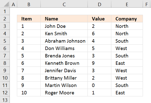
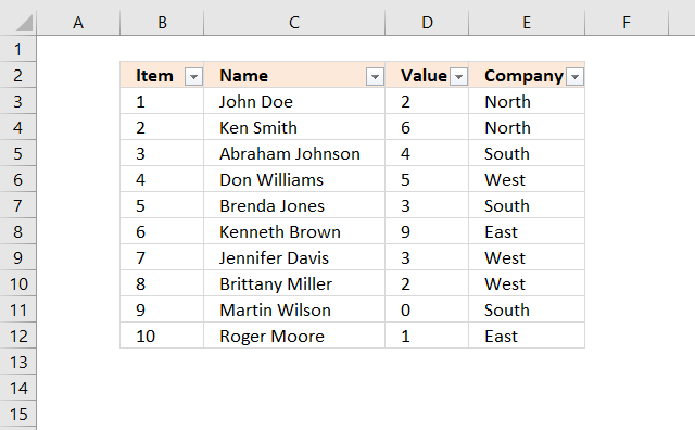
The picture above shows you a dataset in cell range B3:E12, the search parameters are in D14:D16. The search results are in B20:E22.
Cells D14 allows you to specify the start number, and cell D15 is the end number of the range. Cell D16 determines which column to use in cell range B3:E12.
The result is presented in cells B20:E20 and cells below. The example above shows a start value of 4 and an end value of 6, the column is three meaning the third column in cell range B3:E12.
All records that match range 4 to 6 in cell range D3:D12 are extracted, D3:D12 is the third column in B3:E12.
Update 20 Sep 2017, a smaller formula in cell A20.
Array formula in cell A20:
=INDEX($B$3:$E$12, SMALL(IF((INDEX($B$3:$E$12, , $D$16)< =$D$15)*(INDEX($B$3:$E$12, , $D$16)> =$D$14), MATCH(ROW($B$3:$E$12), ROW($B$3:$E$12)), «»), ROWS(B20:$B$20)), COLUMNS($A$1:A1))
Back to top
1.1 Video
See this video to learn more about the formula:
Back to top
1.2 How to enter this array formula
- Select cell A20
- Paste above formula to cell or formula bar
- Press and hold CTRL + SHIFT simultaneously
- Press Enter once
- Release all keys
The formula bar now shows the formula with a beginning and ending curly bracket, that is if you did the above steps correctly. Like this:
{=array_formula}
Don’t enter these characters yourself, they appear automatically.
Now copy cell A20 and paste to cell range A20:E22.
Back to top
1.3 Explaining array formula in cell A20
You can follow along if you select cell A19, go to tab «Formulas» on the ribbon and press with left mouse button on the «Evaluate Formula» button.
Step 1 — Filter a specific column in cell range B3:E12
The INDEX function is mostly used for getting a single value from a given cell range, however, it can also return an entire column or row from a cell range.
This is exactly what I am doing here, the column number specified in cell D16 determines which column to extract.
INDEX($B$3:$E$12, , $D$16, 1)
becomes
INDEX($B$3:$E$12, , 3, 1)
and returns C3:C12.
Recommended articles
Step 2 — Check which values are smaller or equal to the condition
The smaller than and equal sign are logical operators that let you compare value to value, in this case, if a number is smaller than or equal to another number.
The output is a boolean value, True och False. Their positions in the array correspond to the positions in the cell range.
INDEX($B$3:$E$12, , $D$16, 1)< =$D$15
becomes
C3:C12< =$D$15
becomes
{2; 6; 4; 5; 3; 9; 3; 2; 0; 1}<=6
and returns
{TRUE; TRUE; TRUE; TRUE; TRUE; FALSE; TRUE; TRUE; TRUE; TRUE}.
Step 3 — Multiply arrays — AND logic
There is a second condition we need to evaluate before we know which records are in range.
(INDEX($B$3:$E$12, , $D$16, 1)< =$D$15)*(INDEX($B$3:$E$12, , $D$16, 1)> =$D$14)
becomes
({2; 6; 4; 5; 3; 9; 3; 2; 0; 1}< =$C$14)*({2; 6; 4; 5; 3; 9; 3; 2; 0; 1}> =$C$13)
becomes
({2; 6; 4; 5; 3; 9; 3; 2; 0; 1}< =3)*({2; 6; 4; 5; 3; 9; 3; 2; 0; 1}> =0)
becomes
{TRUE; FALSE; FALSE; FALSE; TRUE; FALSE; TRUE; TRUE; TRUE; TRUE}*{TRUE; TRUE; TRUE; TRUE; TRUE; TRUE; TRUE; TRUE; TRUE; TRUE}
Both conditions must be met, the asterisk lets us multiple the arrays meaning AND logic.
TRUE * TRUE equals FALSE, all other combinations return False. TRUE * FALSE equals FALSE and so on.
{TRUE; FALSE; FALSE; FALSE; TRUE; FALSE; TRUE; TRUE; TRUE; TRUE} * {TRUE; TRUE; TRUE; TRUE; TRUE; TRUE; TRUE; TRUE; TRUE; TRUE}
returns
{1; 0; 0; 0; 1; 0; 1; 1; 1; 1}.
Boolean values have numerical equivalents, TRUE = 1 and FALSE equals 0 (zero). They are converted when you perform an arithmetic operation in a formula.
Step 4 — Create number sequence
The ROW function calculates the row number of a cell reference.
ROW(reference)
ROW($B$3:$E$12)
returns
{3; 4; 5; 6; 7; 8; 9; 10; 11; 12}.
Step 5 — Create a number sequence from 1 to n
The MATCH function returns the relative position of an item in an array or cell reference that matches a specified value in a specific order.
MATCH(ROW($B$3:$E$12), ROW($B$3:$E$12))
becomes
MATCH({3; 4; 5; 6; 7; 8; 9; 10; 11; 12}, {3; 4; 5; 6; 7; 8; 9; 10; 11; 12})
and returns
{1; 2; 3; 4; 5; 6; 7; 8; 9; 10}.
Step 6 — Return the corresponding row number
The IF function returns one value if the logical test is TRUE and another value if the logical test is FALSE.
IF(logical_test, [value_if_true], [value_if_false])
IF((INDEX($B$3:$E$12, , $D$16)< =$D$15)*(INDEX($B$3:$E$12, , $D$16)> =$D$14), MATCH(ROW($B$3:$E$12), ROW($B$3:$E$12)), «»)
becomes
IF({1; 0; 0; 0; 1; 0; 1; 1; 1; 1}, MATCH(ROW($B$3:$E$12), ROW($B$3:$E$12)), «»)
becomes
IF({1; 0; 0; 0; 1; 0; 1; 1; 1; 1}, {1; 2; 3; 4; 5; 6; 7; 8; 9; 10}, «»)
and returns
{1; «»; «»; «»; 5; «»; 7; 8; 9; 10}.
Step 7 — Extract k-th smallest row number
The SMALL function returns the k-th smallest value from a group of numbers.
SMALL(array, k)
SMALL(IF((INDEX($B$3:$E$12, , $D$16)< =$D$15)*(INDEX($B$3:$E$12, , $D$16)> =$D$14), MATCH(ROW($B$3:$E$12), ROW($B$3:$E$12)), «»), ROWS(B20:$B$20))
becomes
SMALL({1; «»; «»; «»; 5; «»; 7; 8; 9; 10}, ROWS(B20:$B$20))
becomes
SMALL({1; «»; «»; «»; 5; «»; 7; 8; 9; 10}, 1)
and returns 1.
Step 8 — Return the entire row record from the cell range
The INDEX function returns a value from a cell range, you specify which value based on a row and column number.
INDEX(array, [row_num], [column_num])
INDEX($B$3:$E$12, SMALL(IF((INDEX($B$3:$E$12, , $D$16)< =$D$15)*(INDEX($B$3:$E$12, , $D$16)> =$D$14), MATCH(ROW($B$3:$E$12), ROW($B$3:$E$12)), «»), ROWS(B20:$B$20)), COLUMNS($A$1:A1))
becomes
INDEX($B$3:$E$12, 1, , 1)
and returns {2, «Ken Smith», 6, «North»}.
Back to top
Recommended articles
Back to top
2. Extract all rows from a range based on range criteria — Excel 365
Update 17 December 2020, the new FILTER function is now available for Excel 365 users.
Excel 365 dynamic array formula in cell B20:
=FILTER($B$3:$E$12, (D3:D12<=D15)*(D3:D12>=D14))
It is a regular formula, however, it returns an array of values and extends automatically to cells below and to the right. Microsoft calls this a dynamic array and spilled array.
The array formula below is for earlier Excel versions, it searches for values that meet a range criterion (cell D14 and D15), the formula lets you change the column to search in with cell D16.
This formula can be used with whatever dataset size and shape. To search the first column, type 1 in cell D16. This is a great improvement in both formula size and how easy it is to enter the formula, compared to the array formula in section 1.
Back to top
2.1 Explaining array formula
Step 1 — First condition
The less than character and the equal sign are both logical operators meaning they are able to compare value to value, the output is a boolean value.
In this case, the logical expression evaluates if numbers in D3:D12 are smaller than or equal to the condition specified in cell D15.
D3:D12<=D15
becomes
{2;6;4;5;3;9;3;2;0;1}<=6
and returns
{TRUE; TRUE; TRUE; TRUE; TRUE; FALSE; TRUE; TRUE; TRUE; TRUE}.
Step 2 — Second condition
The second condition checks if the number in D3:D12 are larger than or equal to the condition specified in cell D14.
D3:D12>=D14
becomes
{2;6;4;5;3;9;3;2;0;1}>=4
and returns
{FALSE; TRUE; TRUE; TRUE; FALSE; TRUE; FALSE; FALSE; FALSE; FALSE}.
Step 3 — Multiply arrays — AND logic
The asterisk lets you multiply a number to a number, in this case, array to array. Both arrays must be of the exact same size.
The parentheses let you control the order of operation, we want to evaluate the comparisons first before we multiply the arrays.
(D3:D12<=D15)*(D3:D12>=D14)
becomes
{TRUE; TRUE; TRUE; TRUE; TRUE; FALSE; TRUE; TRUE; TRUE; TRUE}*{FALSE; TRUE; TRUE; TRUE; FALSE; TRUE; FALSE; FALSE; FALSE; FALSE}
and returns
{0; 1; 1; 1; 0; 0; 0; 0; 0; 0}.
AND logic works like this:
TRUE * TRUE = TRUE (1)
TRUE * FALSE = FALSE (0)
FALSE * TRUE = FALSE (0)
FALSE * FALSE = FALSE (0)
Note that multiplying boolean values returns their numerical equivalents.
TRUE = 1 and FALSE = 0 (zero).
Step 4 — Filter values based on the array
The FILTER function lets you extract values/rows based on a condition or criteria.
FILTER(array, include, [if_empty])
FILTER($B$3:$E$12, (D3:D12<=D15)*(D3:D12>=D14))
becomes
FILTER({1, «John Doe», 2, «North»; 2, «Ken Smith», 6, «North»; 3, «Abraham Johnson», 4, «South»; 4, «Don Williams», 5, «West»; 5, «Brenda Jones», 3, «South»; 6, «Kenneth Brown», 9, «East»; 7, «Jennifer Davis», 3, «West»; 8, «Brittany Miller», 2, «West»; 9, «Martin Wilson», 0, «South»; 10, «Roger Moore», 1, «East»}, (D3:D12<=D15)*(D3:D12>=D14))
becomes
FILTER({1, «John Doe», 2, «North»; 2, «Ken Smith», 6, «North»; 3, «Abraham Johnson», 4, «South»; 4, «Don Williams», 5, «West»; 5, «Brenda Jones», 3, «South»; 6, «Kenneth Brown», 9, «East»; 7, «Jennifer Davis», 3, «West»; 8, «Brittany Miller», 2, «West»; 9, «Martin Wilson», 0, «South»; 10, «Roger Moore», 1, «East»}, {0; 1; 1; 1; 0; 0; 0; 0; 0; 0})
and returns
{2, «Ken Smith», 6, «North»; 3, «Abraham Johnson», 4, «South»; 4, «Don Williams», 5, «West»}.
Back to top
3. Extract all rows from a range that meet the criteria in one column [Array formula]
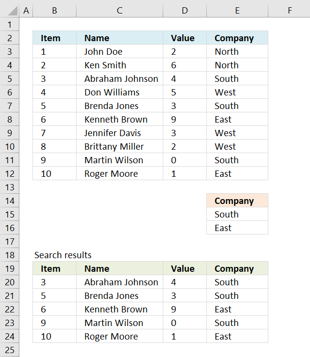
The array formula in cell B20 extracts records where column E equals either «South» or «East». You can use as many conditions as you like as long as you adjust the cell reference $E$15:$E$16 accordingly in the formula below.
The following array formula in cell B20 is for earlier Excel versions than Excel 365:
=INDEX($B$3:$E$12, SMALL(IF(COUNTIF($E$15:$E$16,$E$3:$E$12), MATCH(ROW($B$3:$E$12), ROW($B$3:$E$12)), «»), ROWS(B20:$B$20)), COLUMNS($B$2:B2))
To enter an array formula, type the formula in a cell then press and hold CTRL + SHIFT simultaneously, now press Enter once. Release all keys.
The formula bar now shows the formula with a beginning and ending curly bracket telling you that you entered the formula successfully. Don’t enter the curly brackets yourself.
Back to top
3.1 Explaining formula in cell B20
Step 1 — Filter a specific column in cell range $A$2:$D$11
The COUNTIF function allows you to identify cells in range $E$3:$E$12 that equals $E$15:$E$16.
COUNTIF($E$15:$E$16,$E$3:$E$12)
becomes
COUNTIF({«South»; «East»},{«North»; «North»; «South»; «West»; «South»; «East»; «West»; «West»; «South»; «East»})
and returns
{0;0;1;0;1;1;0;0;1;1}.
Step 2 — Return corresponding row number
The IF function has three arguments, the first one must be a logical expression. If the expression evaluates to TRUE then one thing happens (argument 2) and if FALSE another thing happens (argument 3).
The logical expression was calculated in step 1 , TRUE equals 1 and FALSE equals 0 (zero).
IF(COUNTIF($E$15:$E$16,$E$3:$E$12), MATCH(ROW($B$3:$E$12), ROW($B$3:$E$12)), «»)
becomes
IF({0; 0; 1; 0; 1; 1; 0; 0; 1; 1}, MATCH(ROW($B$3:$E$12), ROW($B$3:$E$12)), «»)
becomes
IF({0; 0; 1; 0; 1; 1; 0; 0; 1; 1}, {1; 2; 3; 4; 5; 6; 7; 8; 9; 10}, «»)
and returns
{«»; «»; 3; «»; 5; 6; «»; «»; 9; 10}.
Step 3 — Find k-th smallest row number
SMALL(IF(COUNTIF($E$15:$E$16,$E$3:$E$12), MATCH(ROW($B$3:$E$12), ROW($B$3:$E$12)), «»), ROWS(B20:$B$20))
becomes
SMALL({«»; «»; 3; «»; 5; 6; «»; «»; 9; 10}, ROWS(B20:$B$20))
becomes
SMALL({«»; «»; 3; «»; 5; 6; «»; «»; 9; 10}, 1)
and returns 3.
Step 4 — Return value based on row and column number
The INDEX function returns a value based on a cell reference and column/row numbers.
INDEX($B$3:$E$12, SMALL(IF(COUNTIF($E$15:$E$16,$E$3:$E$12), MATCH(ROW($B$3:$E$12), ROW($B$3:$E$12)), «»), ROWS(B20:$B$20)), COLUMNS($B$2:B2))
becomes
INDEX($B$3:$E$12, 3, COLUMNS($B$2:B2))
becomes
INDEX($B$3:$E$12, 3, 1)
and returns 3 in cell B20.
Back to top
Recommended articles
Back to top
4. Extract all rows from a range based on multiple conditions — Excel 365
Update 17 December 2020, the new FILTER function is now available for Excel 365 users.
Excel 365 dynamic array formula in cell B20:
=FILTER($B$3:$E$12, COUNTIF(E15:E16, E3:E12))
It is a regular formula, however, it returns an array of values. Read here how it works: Filter values based on criteria
The formula extends automatically to cells below and to the right. Microsoft calls this a dynamic array and spilled array.
Back to top
4.1 Explaining array formula
Step 1 — Check if values equal criteria
The COUNTIF function calculates the number of cells that meet a given condition.
COUNTIF(range, criteria)
COUNTIF($E$15:$E$16,$E$3:$E$12)
becomes
COUNTIF({«South»; «East»},{«North»; «North»; «South»; «West»; «South»; «East»; «West»; «West»; «South»; «East»})
and returns
{0; 0; 1; 0; 1; 1; 0; 0; 1; 1}.
Step 2 — Filter records based on array
The FILTER function lets you extract values/rows based on a condition or criteria.
FILTER(array, include, [if_empty])
FILTER($B$3:$E$12, COUNTIF(E15:E16, E3:E12))
becomes
FILTER($B$3:$E$12, {0; 0; 1; 0; 1; 1; 0; 0; 1; 1})
and returns
{3, «Abraham Johnson», 4, «South»; 5, «Brenda Jones», 3, «South»; 6, «Kenneth Brown», 9, «East»; 9, «Martin Wilson», 0, «South»; 10, «Roger Moore», 1, «East»}.
Back to top
5. Extract all rows from a range that meet the criteria in one column [Excel defined Table]
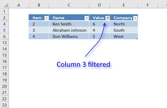
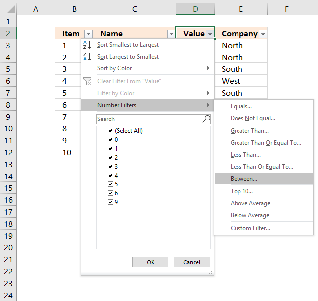
The image above shows a dataset converted to an Excel defined Table, a number filter has been applied to the third column in the table.
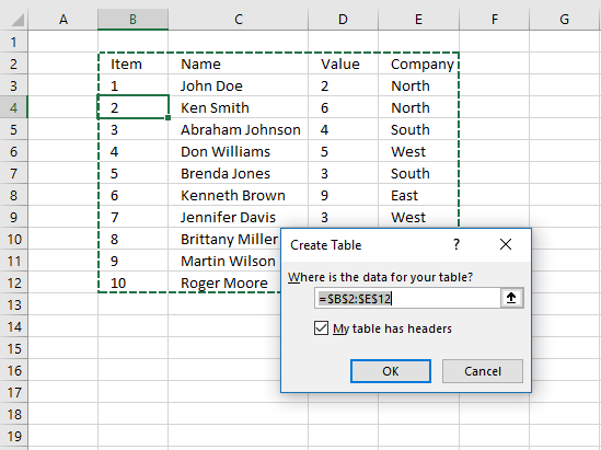
Here are the instructions to create an Excel Table and filter values in column 3.
- Select a cell in the dataset.
- Press CTRL + T

- Press with left mouse button on check box «My table has headers».
- Press with left mouse button on OK button.

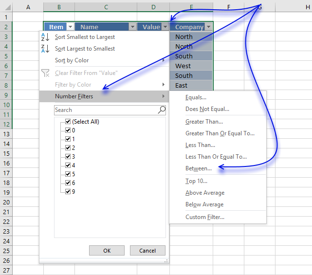
The image above shows the Excel defined Table, here is how to filter D between 4 and 6:
- Press with left mouse button on black arrow next to header.
- Press with left mouse button on «Number Filters».
- Press with left mouse button on «Between…».

- Type 4 and 6.

- Press with left mouse button on OK button.

Back to top
6. Extract all rows from a range that meet the criteria in one column [AutoFilter]
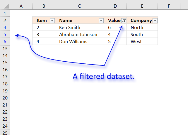
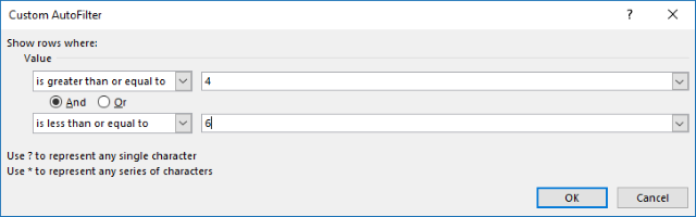
The image above shows filtered records based on two conditions, values in column D are larger or equal to 4 or smaller or equal to 6.
Here is how to apply Filter arrows to a dataset.
- Select any cell within the dataset range.
- Go to tab «Data» on the ribbon.
- Press with left mouse button on «Filter button».

Black arrows appear next to each header.
Lets filter records based on conditions applied to column D.
- Press with left mouse button on the black arrow next to the header in Column D, see the image below.
- Press with left mouse button on «Number Filters».
- Press with left mouse button on «Between».

- Type 4 and 6 in the dialog box shown below.
- Press with left mouse button on OK button.
Back to top
7. Extract all rows from a range that meet the criteria in one column
[Advanced Filter]
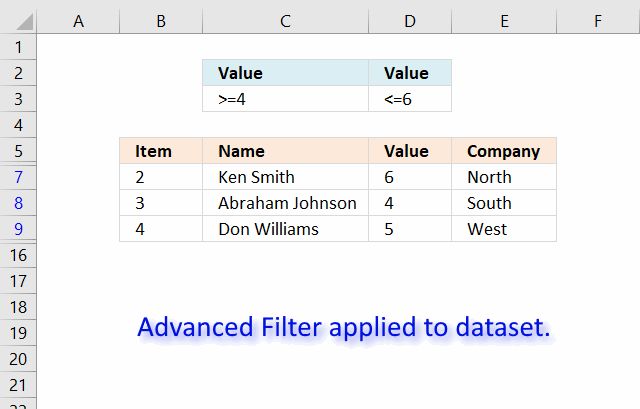
The image above shows a filtered dataset in cell range B5:E15 using Advanced Filter which is a powerful feature in Excel.
Here is how to apply a filter:
- Create headers for the column you want to filter, preferably above or below your data set.
Your filters will possibly disappear if placed next to the data set because rows may become hidden when the filter is applied. - Select the entire dataset including headers.
- Go to tab «Data» on the ribbon.
- Press with left mouse button on the «Advanced» button.

- A dialog box appears.

- Select the criteria range C2:D3, shown ithe n above image.
- Press with left mouse button on OK button.
Back to top
Recommended articles
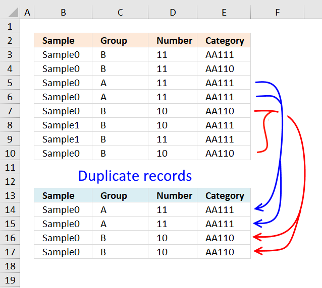
Extract duplicate records
This article describes how to filter duplicate rows with the use of a formula. It is, in fact, an array […]
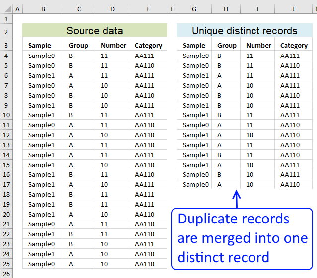
Filter unique distinct records
Table of contents Filter unique distinct row records Filter unique distinct row records but not blanks Filter unique distinct row […]
Back to top
8. Excel file
Back to top
How to extract specific rows in Excel?
Filter unique entries
- Select a cell in the database.
- On the Data tab of the Excel ribbon, click Advanced.
- In the Advanced Filter dialog, select Copy to another place.
- In the list area, select the column or columns from which you want to extract unique values.
- Leave the criteria field blank.
How to extract multiple rows of matching criteria in Excel?
This is an array formula and must be entered with Ctrl + Shift + Enter. After entering the formula in the first cell, drag it down and up to fill the other cells.
How to isolate rows in Excel?
To hide unused rows in Excel 2003, select a row in the Last Row section of the worksheet. (Select the row header to select the entire row.) Then press CTRL + SHIFT + DOWN ARROW to select each row between the selected row and the bottom of the worksheet. Then choose Line from the Format menu and choose Hide.
What is the best way to select a row with a specific value in an Excel column?
Select cells, entire rows, or entire columns that contain specific text or value
- Select the range from which you want to select cells, entire rows, or entire columns. …
- Go to the “Select Specific Cells” dialog box and in the “Select Type” section, specify the desired option.
How to select rows in Excel based on criteria?
Mark rows based on multiple criteria
- Select the entire entry (in this example A2:F17).
- Open the Home tab.
- In the Styles group, click Conditional Formatting.
- Click New Rules.
- In the New Format Rule dialog box, click Use formula to define cells to format.
How to extract a dynamic list in Excel with multiple criteria?
How to copy alternate rows in Excel?
Copy all other rows in Excel with fill stitch
- Copy all the other lines to stand out with the fill stitch. …
- Step 2 – Select and select the area E1:G2, then drag the fill handle over the area as needed. …
- Note. This method only copies the content of each line, without hyperlinks, formatting styles, etc.
How to combine data in Excel?
Click Data > Consolidate (in the Data Tools group). In the Function field, click the resulting function that you want to use to consolidate data in Excel. The default function is SUM. Select the dates.
How to highlight a large number of cells in Excel without scrolling?
Selection of a wide range of data in Excel
- Click on the cell in the upper left corner of the panel.
- Click in the Name field and enter the cell in the lower right corner of the range.
- Press SHIFT + Enter.
- Excel selects the entire range.
How can I extract data from multiple criteria in Excel?
We use INDEX MATCH functions with multiple criteria following these 5 steps:
- Step 1: understand the basics.
- Step 2. Enter the usual MATCH RATE formula.
- Step 3 – Change the lookup value to 1.
- Step 4: Enter the criteria.
- Step 5: Ctrl + Shift + Enter.
How to filter rows in Excel based on cell value?
Filter the data range
- Select any cell in the range.
- Choose Data > Filter.
- Select the arrow in the column header.
- Select “Text Filter” or “Number Filter” and then choose the comparison, e.g. B. “Enter.”
- Enter the filter criteria and click OK.
I have a sheet with a number of columns. One of them lists different dates in a format of »Planned dd/mm/yyyy». The dates range from 2003 until 2011. I only need those from 2010 and 2011.
What I want to do is to find the values with 2010 and 2011 in that column and copy paste them along with the respective rows to another sheet.
I would highly appreciate any help.
asked Oct 21, 2011 at 8:30
![]()
2
Once you have removed «Planned » from the data and changed the column into date format (as per your comment) then you can select all the rows in the sheet and choose Data > Sort from the menu to sort the sheet by the date column (make sure «No Header Row» is selected). It should then be easy enough to select all rows in 2010/2011, since they are now contiguous, and copy them to another sheet.
answered Oct 21, 2011 at 8:54
![]()
MrWhiteMrWhite
2,8084 gold badges31 silver badges43 bronze badges
0
Assume that you’re in a situation where you need to filter every nth row from a list having a few values. I’m pretty sure you’d choose to do it manually, which is also a great choice when you only have a few values in a list and want to filter out every nth row.
However, if you are dealing with several values in the list and want to filter out the nth row, then executing these jobs manually would be a stupid move since there is a 90% probability that you will become tired of it and will be unable to accomplish your assignment on time.
But don’t worry, after carefully reading this post, filtering off every nth row from a list with multiple values will be a piece of cake for you.

So let’s go into the article and get you out of this bind.
Table of Contents
- The formula in General
- Explanations of Syntax
- Let’s See How This Formula Works
- Related Functions
The formula in General
In MS Excel, use the following formula to filter every nth row:
=FILTER(total_data,MOD(SEQUENCE(ROWS(total_data)),n)=0)
Explanations of Syntax
Before we get into the formula for getting the job done quickly, we need to grasp each syntax to see how each syntax helps filter out every nth row in MS Excel.
-
Filter: This tool helps narrow down or filter out a range of data based on user-defined criteria. -
Comma symbol (,): In Excel, this comma symbol serves as a separator, aiding in separating a list of values. total_data: is nothing more than representing each column in the list.Parenthesis(): The primary function of this Parenthesis symbol is to group and separate elements.ROWS: This refers to the nth row you want to filter out.MOD(): The MOD function accepts two real number operands as inputs and returns the remainder of dividing the integer component of the first parameter (the dividend) by the integer part of the second argument (the divisor)SEQUENCE(): The SEQUENCE function in Excel lets you create a sequence of consecutive numbers in an array, such as 1, 2, 3, 4.
Let’s See How This Formula Works
For example, suppose you have a task in which there is a table with candidates from two regions (i.e., West and East ) and which are assigned to a particular sales number; now you want to filter out every second row, which is the sequence which we would write in the formula; now let’s analyze how to write the formula and how this formula would do it.
To filter every second row, we would use the following formula based on the supplied list:
=FILTER(A2:C10,MOD(SEQUENCE(ROWS(A2:C10)),2)=0)
To filter and extract every nth row, use a formula that combines the FILTER function with MOD, ROW, and SEQUENCE. Where data refers to the designated range A2:C10. With n hardcoded as 2, the FILTER function retrieves every third row in the data.
The FILTER function filters and extracts data based on logical criteria. This example aims to extract every second record from the supplied data, although there is no row number information in the data range A2:C10.
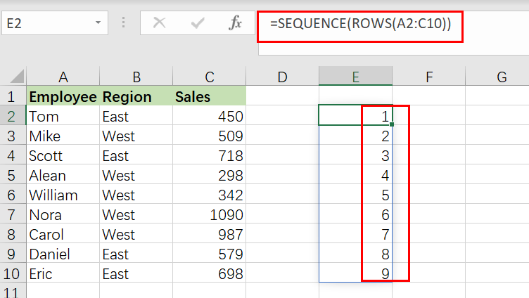
The first stage, working from the inside out, is establishing a row number set. This is accomplished using the SEQUENCE function as follows:
=SEQUENCE(ROWS(A2:C10))
The ROW function returns the number of rows in the specified range of data. SEQUENCE provides an array of 9 integers in sequence based on the number of rows:
{1;2;3;4;5;6;7;8;9}
This array is sent straight to the MOD function as the number parameter, with the divisor hardcoded as 2. MOD is configured to check if row numbers are divisible by 2 with a remainder of zero.
=MOD(SEQUENCE(ROWS(A2:C10)),2)=0 /// is it divisible by 2?
MOD produces an array of TRUE and FALSE values, as shown below:
{FALSE;TRUE;FALSE;TRUE;FALSE;TRUE;FALSE;TRUE;FALSE}
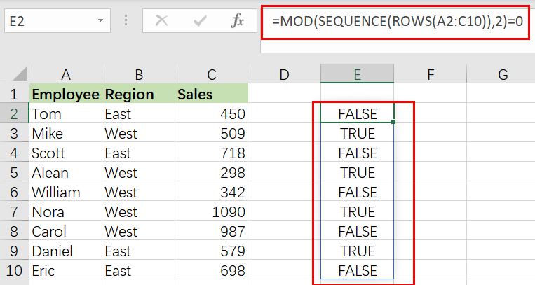
Take note that TRUE values correlate to every second row in the data range A2:C10. This array is passed straight to the FILTER function as the include parameter. As a final result, FILTER returns every second row of data.
- Excel Filter function
The Excel FILTER function extracts matched records from a collection of data using one or more logical checks. The include argument specifies logical tests, which might encompass a wide variety of formula conditions.==FILTER(array,include,[if empty])… - Excel MOD function
the Excel MOD function returns the remainder of two numbers after division. So you can use the MOD function to get the remainder after a number is divided by a divisor in Excel. The syntax of the MOD function is as below:=MOD (number, divisor)…. - Excel ROWS function
The Excel ROWS function returns the number of rows in a cell reference.The syntax of the ROWS function is as below:= ROWS(array)…
Here is a solution with array formulas. It will calculate extremely slowly, and honestly VBA is a much better solution. You will need to tell excel these are array formulas by hitting «Ctrl + Shift + Enter» after inputting the formulas, this will add the {} around the equation. Finally, drag down the array formulas to see the first «X» results with blood type «O»:
First cell formula for «Blood» —> assumes blood is in column A of sheet1
{=IFERROR(INDEX(Sheet1!$A:$D,SMALL(IF(Sheet1!$A:$A="O",ROW(Sheet1!$A:$A)),ROW(1:1)),1,1),"")}
First cell formula for «Name» —> assumes name is in column B of sheet1
{=IFERROR(INDEX(Sheet1!$A:$D,SMALL(IF(Sheet1!$A:$A="O",ROW(Sheet1!$A:$A)),ROW(1:1)),2,1),"")}
First cell formula for «Age» —> assumes age is in column c of sheet1
{=IFERROR(INDEX(Sheet1!$A:$D,SMALL(IF(Sheet1!$A:$A="O",ROW(Sheet1!$A:$A)),ROW(1:1)),3,1),"")}
First cell formula for «Gender» —> assumes gender is in column d of sheet1
{=IFERROR(INDEX(Sheet1!$A:$D,SMALL(IF(Sheet1!$A:$A="O",ROW(Sheet1!$A:$A)),ROW(1:1)),4,1),"")}
Results:
BLOOD   NAME    AGE GENDER
O       Lucy    32  Female
O       John    11  Male
O       Amy     23  Female
O       Linda   11  Female