
Хитрости »
1 Май 2011 398148 просмотров
Как оставить в ячейке только цифры или только текст?
Вот бывает так: есть у Вас в ячейке некий текст. Допустим «Было доставлено кусков мыла 763шт.». Вам нужно из этого только 763 — чтобы можно было провести с этим некие математические действия. Если это только одна ячейка — проблем тут нет, а если таких ячеек пару тысяч? И к тому же все разные?
- Было доставлено кусков мыла 763шт.
- Всего пришло 34
- Тюбики — 54 доставлено
- и т.д.
Никакой зацепки для извлечения данных. Пару тысяч таких строк удалять вручную весьма утомительное занятие, надо сказать. Да еще и не быстрое.
Есть несколько вариантов решения подобной задачи.
СПОСОБ 1: не используем макросы
можно применить формулу массива, вроде такой:
=ПСТР(A1;МИН(ЕСЛИ(ЕЧИСЛО(-ПСТР(A1;СТРОКА($1:$99);1));СТРОКА($1:$99)));ПРОСМОТР(2;1/ЕЧИСЛО(-ПСТР(A1;СТРОКА($1:$99);1));СТРОКА($1:$99))-МИН(ЕСЛИ(ЕЧИСЛО(-ПСТР(A1;СТРОКА($1:$99);1));СТРОКА($1:$99)))+1)
Три важных момента:
- Формула вводится в ячейку сочетанием клавиш Ctrl+Shift+Enter, т.к. является формулой массива. Подробнее про эти формулы читайте в статье: Что такое формула массива
- в таком виде формула работает с текстом, количество символов в котором не превышает 99. Чтобы расширить необходимо в формуле во всех местах заменить СТРОКА($1:$99) на СТРОКА($1:$200). Т.е. вместо 99 указать количество символов с запасом. Только не увлекайтесь, иначе может получиться, что формула будет работать слишком долго
- формула не обработает корректно текст «Было доставлено кусков мыла 763шт., а заказывали 780» и ему подобный, где числа раскиданы по тексту.
Теперь коротко разберем формулу на примере фразы: Было доставлено кусков мыла 763шт.
- в A1 сам текст, из которого необходимо извлечь числа: Было доставлено кусков мыла 763шт., а заказывали 780
- блок: МИН(ЕСЛИ(ЕЧИСЛО(-ПСТР(A1;СТРОКА($1:$99);1));СТРОКА($1:$99)))
вычисляет позицию первой цифры в ячейке — 29 - блок: ПРОСМОТР(2;1/ЕЧИСЛО(-ПСТР(A1;СТРОКА($1:$99);1));СТРОКА($1:$99))
вычисляет позицию последней цифры в ячейке — 31 - в результате получается: =ПСТР(A1;29;31—29+1)
функция ПСТР извлекает из текста, указанного первым аргументом(A1) текст, начиная с указанной позиции(29) с количеством символов, указанным третьим аргументом(31—29+1) - И в итоге:
=ПСТР(A1;29;31—29+1)
=> =ПСТР(A1;29;2+1)
=> =ПСТР(A1;29;3)
=> 763
Может быть задача проще — необходимо извлечь односоставной текст, убрав цифры вначале и в конце строки, учитывая, что сам текст всегда следует после разделителя(например, тире):
12.08-АГСВ2
12.08-АГСВ1
01.03-ОВ2
12.03-КЖ6.1
Из этих данных надо получить только текст после тире(-) и отсечь цифры на конце:
АГСВ
АГСВ
ОВ
КЖ
Формула будет работать почти по тому же принципу, что и формула выше, но она проще:
=ПСТР(A1;ПОИСК(«-«;A1)+1;ПОИСКПОЗ(ИСТИНА;ЕЧИСЛО(—ПСТР(ПСТР(A1;ПОИСК(«-«;A1)+1;999);СТРОКА($1:$99);1));0)-1)
В данном случае мы при помощи
ПОИСК(«-«;A1)
ищем сначала позицию тире, далее при помощи
ПОИСКПОЗ(ИСТИНА;ЕЧИСЛО(—ПСТР(ПСТР(A1;ПОИСК(«-«;A1)+1;999);СТРОКА($1:$99);1));0)
находим именно в отсеченном тексте позицию первой цифры. Передаем эти значения в
ПСТР
, которая отбирает из этого текста все от первого тире(+1) до первого числа, идущего после текста.
СПОСОБ 2: используем макросы
Самый главный недостаток метода при помощи формулы, приведенной выше — из текста «Было доставлено кусков мыла 763шт., а заказывали 780» формула вернет не только числа, а и текст между первой и последней цифрой: 763шт., а заказывали 780.
Решить же проблему извлечения цифр даже из такого текста при помощи VBA куда проще и гибче. Плюс можно не только цифры извлекать, но и наоборот — цифры удалить, а извлечь только текст. Ниже приведен код пользовательской функции, которая поможет извлечь из строки только числа либо только текст. Иными словами, результатом функции будет либо только текст, либо только числа.
Function Extract_Number_from_Text(sWord As String, Optional Metod As Integer)
'sWord = ссылка на ячейку или непосредственно текст
'Metod = 0 – числа
'Metod = 1 – текст
    Dim sSymbol As String, sInsertWord As String
    Dim i As Integer

    If sWord = "" Then Extract_Number_from_Text = "Нет данных!": Exit Function
    sInsertWord = ""
    sSymbol = ""
    For i = 1 To Len(sWord)
        sSymbol = Mid(sWord, i, 1)
        If Metod = 1 Then
            If Not LCase(sSymbol) Like "*[0-9]*" Then
                If (sSymbol = "," Or sSymbol = "." Or sSymbol = " ") And i > 1 Then
                    If Mid(sWord, i - 1, 1) Like "*[0-9]*" And Mid(sWord, i + 1, 1) Like "*[0-9]*" Then
                        sSymbol = ""
                    End If
                End If
                sInsertWord = sInsertWord & sSymbol
            End If
        Else
            If LCase(sSymbol) Like "*[0-9.,;:-]*" Then
                If LCase(sSymbol) Like "*[.,]*" And i > 1 Then
                    If Not Mid(sWord, i - 1, 1) Like "*[0-9]*" Or Not Mid(sWord, i + 1, 1) Like "*[0-9]*" Then
                        sSymbol = ""
                    End If
                End If
                sInsertWord = sInsertWord & sSymbol
            End If
        End If
    Next i
    Extract_Number_from_Text = sInsertWord
End Function
Чтобы правильно использовать приведенный код, необходимо сначала ознакомиться со статьей Что такое функция пользователя(UDF)?. Вкратце: скопировать текст кода выше, перейти в редактор VBA(Alt+F11) -создать стандартный модуль(Insert —Module) и в него вставить скопированный текст. После чего функцию можно будет вызвать из Диспетчера функций(Shift+F3), отыскав её в категории Определенные пользователем (User Defined Functions) и применять как обычную функцию на листе.
Для извлечения только чисел
=Extract_Number_from_Text(A1; 0)
или
=Extract_Number_from_Text(A1)
Для извлечения только текста
=Extract_Number_from_Text(A1; 1)
Подробнее про создание пользовательских функции и их применении можно почитать в статье Что такое функция пользователя(UDF)?
Помимо функции пользователя решил выложить и вариант с использованием диалогового окна:

Выбрать ячейку или диапазон с текстом(Лист1!$A$2:$A$10) — здесь указывается диапазон с исходными значениями, из которого необходимо оставить только числа или только текст.
Выберите ячейку для вывода данных(Лист1!$A$2) — указывается одна ячейка, с которой начать вывод преобразованных значений. В качестве этой ячейки можно выбрать первую ячейку диапазона с текстом(исходного) если необходимо произвести изменения сразу в этих же ячейках(как на рисунке). Осторожнее с таким указанием, т.к. результат работы кода может быть не совсем таким, какой вы ожидали, а вернуть прежние данные уже не получится — если только не закрыть файл без сохранения изменений.
Оставить только цифры, Оставить только текст— думаю не надо пояснять. Здесь выбираем, что оставить в качестве результата.
Небольшое дополнение к использованию кода
В коде есть строка:
If LCase(sSymbol) Like "*[0-9.,;:-]*" Then
Данная строка отвечает за текстовые символы, которые могут встречаться внутри чисел и которые надо оставить(не удалять наравне с другими не числовыми символами). Следовательно, если какие-то из данных символов не нужны в конечном тексте — их надо просто удалить. Например, чтобы оставались исключительно числа(без запятых и пр.):
If LCase(sSymbol) Like "*[0-9]*" Then
если надо исключить из удаления помимо цифр точку(т.е. будут извлечены цифры и точка):
If LCase(sSymbol) Like "*[0-9.]*" Then
и т.д.
Скачать пример:
 Число из текста и наоборот.xls (99,0 KiB, 17 666 скачиваний)
Также см.:
Извлечение числа из текста
Что такое функция пользователя(UDF)?
Как получить адрес гиперссылки из ячейки
Оставить цифры или текст при помощи PowerQuery
Статья помогла? Поделись ссылкой с друзьями!
![]() Видеоуроки
Видеоуроки
Поиск по меткам
Access
apple watch
Multex
Power Query и Power BI
VBA управление кодами
Бесплатные надстройки
Дата и время
Записки
ИП
Надстройки
Печать
Политика Конфиденциальности
Почта
Программы
Работа с приложениями
Разработка приложений
Росстат
Тренинги и вебинары
Финансовые
Форматирование
Функции Excel
акции MulTEx
ссылки
статистика
Skip to content
В этом кратком руководстве показано, как можно быстро извлекать число из различных текстовых выражений в Excel с помощью формул или специального инструмента «Извлечь».
Проблема выделения числа из текста возникает достаточно часто, особенно когда вы работаете с данными, полученными из других программ. К примеру, нужно вытащить почтовый индекс из адреса, номенклатурный номер из строки с наименованием товара, номер счета из платежного документа. Нужное нам число может находиться в любом месте текста — в начале, в середине или в конце.
Вот что мы рассмотрим в этой статье:
- Как извлечь число в конце текста
- Получаем число из начала текста
- Как извлечь все числа из текста
- Извлекаем числа без формул при помощи Ultimate Suite
Когда дело доходит до извлечения части текстового значения заданной длины, Эксель предоставляет три текстовых функции (ЛЕВСИМВ, ПРАВСИМВ и ПСТР) для быстрого выполнения этой задачи. А вот когда дело доходит до извлечения числа из буквенно-цифровой строки, Microsoft Excel … не предоставляет ничего.
Чтобы извлечь число из текста в Excel, требуется немного изобретательности, немного терпения и множество различных функций, вложенных друг в друга.
Или вы можете запустить инструмент «Извлечь (Extract)» из надстройки Ablebits Ultimate Suite и выполнить эту операцию одним щелчком мыши. Ниже вы найдете полную информацию обо всех этих методах.
Как извлечь число из конца текстовой строки.
Если у вас есть столбец буквенно-цифровых значений, в котором число всегда идет после текста, вы можете использовать одну из следующих формул, чтобы вытащить из них числа.
Важное замечание! В приведенных ниже формулах извлечение выполняется с помощью функций ПРАВСИМВ и ЛЕВСИМВ, которые относятся к категории текстовых функций. Эти функции всегда возвращают текст. В нашем случае результатом будет числовая подстрока, которая с точки зрения Excel также является текстом, а не числом. Если вам нужно, чтобы результат был числом (которое можно использовать в дальнейших вычислениях), оберните соответствующую формулу в функцию ЗНАЧЕН, или выполните с ней простейшую математическую операцию (например, двойное отрицание).
Чтобы извлечь число из строки «текстовое число», первое, что вам нужно знать, — это с какой позиции начать операцию. Итак, давайте определим положение первой цифры с помощью этой общего выражения:
=МИН(ПОИСК({0;1;2;3;4;5;6;7;8;9}; ячейка &»0123456789″))
О логике вычислений мы поговорим чуть позже. На данный момент просто замените слово «ячейка» ссылкой на позицию, содержащую исходный текст (в нашем случае A2), и запишите получившееся выражение в любую пустую клетку той же строки, скажем, в B2:
=МИН(ПОИСК({0;1;2;3;4;5;6;7;8;9};A2&»0123456789″))
Хотя формула содержит константу массива, это обычное выражение, которое вводится обычным способом: нажатием клавиши Enter.
Как только позиция первой цифры определена, можно использовать функцию ПРАВСИМВ для извлечения числа. Чтобы узнать, сколько символов нужно извлечь, вы вычитаете позицию первой цифры из общей длины строки и добавляете единицу к результату, потому что первая цифра также должна быть включена:
=ПРАВСИМВ(A2;ДЛСТР(A2)-B2+1)
Где A2 — исходная ячейка, а B2 — позиция первой цифры.
На следующем скриншоте показаны результаты:

Чтобы исключить вспомогательный столбец, содержащий позицию первой цифры, вы можете встроить формулу МИН непосредственно в функцию ПРАВСИМВ следующим образом:
=ПРАВСИМВ(A2;ДЛСТР(A2)-МИН(ПОИСК({0;1;2;3;4;5;6;7;8;9};A2&»0123456789″))+1)
Чтобы формула возвращала именно число, а не числовую строку, вложите ее в функцию ЗНАЧЕН:
=ЗНАЧЕН(ПРАВСИМВ(A2;ДЛСТР(A2)-МИН(ПОИСК({0;1;2;3;4;5;6;7;8;9};A2&»0123456789″))+1))
Или просто примените двойное отрицание, использовав два знака «минус»:
=—ПРАВСИМВ(A2;ДЛСТР(A2)-МИН(ПОИСК({0;1;2;3;4;5;6;7;8;9};A2&»0123456789″))+1)
Другой способ извлечь число из конца строки — использовать вот такое выражение:
=ПРАВСИМВ( ячейка ;СУММ(ДЛСТР( ячейка ) — ДЛСТР(ПОДСТАВИТЬ( ячейка ; {«0″;»1″;»2″;»3″;»4″;»5″;»6″;»7″;»8″;»9″};»»))))
Используя исходный текст в A2, вы записываете приведенную ниже формулу в B2 или любую другую пустую ячейку в той же строке, а затем копируете её вниз по столбцу:
=ПРАВСИМВ(A2;СУММ(ДЛСТР(A2) — ДЛСТР(ПОДСТАВИТЬ(A2; {«0″;»1″;»2″;»3″;»4″;»5″;»6″;»7″;»8″;»9″};»»))))

Примечание. Эти формулы предназначены для случая, когда числа находятся только в конце текстовой строки. Если некоторые цифры также находятся в середине или в начале, то ничего не будет работать.
Этих недостатков не имеет третья формула, которая извлекает только последнее число в тексте, игнорируя все предыдущие:
=ПРАВСИМВ(A2; ДЛСТР(A2) — МАКС(ЕСЛИ(ЕЧИСЛО(ПСТР(A2; СТРОКА(ДВССЫЛ( «1:»&ДЛСТР(A2))); 1) *1)=ЛОЖЬ; СТРОКА(ДВССЫЛ( «1:»&ДЛСТР(A2))); 0)))
На скриншоте ниже вы видите результат ее работы.

Как видите, цифры в начале или в середине текста игнорируются. Также обратите внимание, что результатом, как и в предыдущих формулах, является число, записанное в виде текста. Как превратить его в нормальное число, мы уже рассмотрели выше в этой статье.
Примечание. Если вы используете Excel 2019 или более ранние версии, нужно использовать формулу массива, нажав при вводе комбинацию Ctrl+Shift+Enter. Если у вас Office365, вводите как обычно, через Enter.
Как извлечь число из начала текстовой строки
Если вы работаете со строками, в которых текст находится после числа, решение для извлечения числа будет аналогично описанному выше. С той только разницей, что вы используете функцию ЛЕВСИМВ для извлечения из левой части текста:
=ЛЕВСИМВ( ячейка ;СУММ(ДЛСТР( ячейка )-ДЛСТР(ПОДСТАВИТЬ( ячейка ;{«0″;»1″;»2″;»3″;»4″;»5″;»6″;»7″;»8″;»9″};»»))))
Используя этот метод для A2, извлекаем число при помощи такого выражения:
=ЛЕВСИМВ(A2;СУММ(ДЛСТР(A2)-ДЛСТР(ПОДСТАВИТЬ(A2;{«0″;»1″;»2″;»3″;»4″;»5″;»6″;»7″;»8″;»9″};»»))))

Это решение работает для текстовых выражений, которые содержат числа только в начале. Если некоторые цифры также находятся в середине или в конце строки, формула не будет работать.
Если вы хотите извлечь только числа слева и игнорировать остальные, воспользуйтесь другой формулой:
=ЛЕВСИМВ(A2;ПОИСКПОЗ(ЛОЖЬ;ЕЧИСЛО(—ПСТР(A2;СТРОКА($1:$94);1));0)-1)
Или чуть модифицируем, чтобы ускорить расчеты:
=ЛЕВСИМВ(A2; ПОИСКПОЗ(ЛОЖЬ; ЕЧИСЛО(ПСТР(A2; СТРОКА(ДВССЫЛ( «1:»&ДЛСТР(A2)+1)); 1) *1); 0) -1)

Если у вас Excel 2019 и ниже, вводите ее как формулу массива, используя Ctrl+Shift+Enter. В Office365 и выше можно вводить как обычно.
Примечание. Как и в случае с функцией ПРАВСИМВ, функция ЛЕВСИМВ также возвращает числовую подстроку, которая технически является текстом, а не числом.
Как получить число из любой позиции в тексте
Если ваша задача подразумевает извлечение числа из любого места строки, вы можете использовать следующую формулу:
=СУММПРОИЗВ(ПСТР(0&A2; НАИБОЛЬШИЙ(ИНДЕКС(ЕЧИСЛО(—ПСТР(A2; СТРОКА(ДВССЫЛ(«1:»&ДЛСТР(A2))); 1)) * СТРОКА(ДВССЫЛ(«1:»&ДЛСТР(A2))); 0); СТРОКА(ДВССЫЛ(«1:»&ДЛСТР(A2))))+1; 1) * 10^СТРОКА(ДВССЫЛ(«1:»&ДЛСТР(A2)))/10)
Где A2 — исходная текстовая строка.
Для пояснения, как это работает, потребуется отдельная статья. Поэтому вы можете просто скопировать на свой рабочий лист, чтобы убедиться, что это действительно работает 

Обратите внимание, что в этом случае в тексте могут находиться несколько чисел. Все они будут извлечены и объединены в единое целое.
Однако, изучив результаты, вы можете заметить один незначительный недостаток: если исходный текст в ячейке не содержит числа, формула возвращает ноль, как в строке 7 на скриншоте выше. Чтобы исправить это, вы можете заключить формулу в оператор ЕСЛИ, который проверит, содержит ли исходный текст какое-либо число. Если это так, формула извлекает это число, в противном случае возвращает пустую строку:
=ЕСЛИ(СУММ(ДЛСТР(A2)-ДЛСТР(ПОДСТАВИТЬ(A2;{«0″;»1″;»2″;»3″;»4″;»5″;»6″;»7″;»8″;»9″};»»)))>0; СУММПРОИЗВ(ПСТР(0&A2; НАИБОЛЬШИЙ(ИНДЕКС(ЕЧИСЛО(—ПСТР(A2; СТРОКА(ДВССЫЛ(«1:»&ДЛСТР(A2))); 1)) * СТРОКА(ДВССЫЛ(«1:»&ДЛСТР(A2))); 0); СТРОКА(ДВССЫЛ(«1:»&ДЛСТР(A2))))+1; 1) * 10^СТРОКА(ДВССЫЛ(«1:»&ДЛСТР(A2)))/10);»»)
В отличие от всех предыдущих примеров, результатом этих формул является число. Чтобы убедиться в этом, просто обратите внимание на выровненные по правому краю значения в столбце B и усеченные ведущие нули (например, 88 вместо 088).
Если число, которое вы хотите извлечь, ограничено какими-то знаками-разделителями, то можно использовать функцию ПСТР. Рассмотрим пример, как получить номер счета из текста платежа.
Мы будем искать позицию знака «№» и позицию следующего за ним первого пробела. То, что находится между ними, как раз и будет номером счёта:
=ПСТР(ПОДСТАВИТЬ(A2;» «;»»);НАЙТИ(«№»;ПОДСТАВИТЬ(A2;» «;»»))+1;НАЙТИ(» «;A2;НАЙТИ(«№»;A2;1))-НАЙТИ(«№»;A2;1)-1)
На скриншоте ниже вы видите, как это работает.

Вот еще один возможный вариант вынимания числа из текста. Необходимо извлечь первое встретившееся число из текста.
Используем формулу
=ПРОСМОТР(2^64;—ЛЕВСИМВ(ПСТР(A1&»_0″;МИН(НАЙТИ({0;1;2;3;4;5;6;7;8;9};A1&»_0123456789″));15); {1;2;3;4;5;6;7;8;9;10;11;12;13;14;15}))
или заменяем список цифр функцией:
=ПРОСМОТР(2^64;—ЛЕВСИМВ(ПСТР(A1&»_0″;МИН(НАЙТИ({0;1;2;3;4;5;6;7;8;9};A1&»_0123456789″));15); СТРОКА($A$1:$IV$16)))
Как видите, получаем только первое число, независимо от его расположения:

И еще один пример. Давайте попробуем достать все числа из текста, разграничив их каким-то разделителем. Например, дефисом “-“.
В этом случае придется использовать формулу массива:
{=ПОДСТАВИТЬ(СЖПРОБЕЛЫ(СЦЕП(ЕСЛИ(ЕЧИСЛО(—ПСТР(A2;СТРОКА($1:$94);1));ПСТР(A2;СТРОКА($1:$94);1);» «)));» «;»-«)}
Мы нашли все числа в тексте, как вы видите на скриншоте ниже:

Откорректировав эту формулу, вы можете использовать любой другой разделитель.
Поскольку между ними есть разделители, то вы легко можете распределить эти числа в отдельные ячейки. Как это сделать — читайте в материале 8 способов разделить ячейку Excel на две или несколько.
Как выделить число из текста с помощью Ultimate Suite
Как вы только что видели, не существует простой и понятной формулы Excel для извлечения чисел из текстовой строки. Если у вас есть трудности с пониманием формул или их настройкой для ваших наборов данных, вам может понравиться этот простой способ получить число из текста в Excel.
С надстройкой Ultimate Suite, добавленной на вашу ленту Excel, вы можете быстро получить число из любой буквенно-цифровой строки:
- Перейдите на вкладку Ablebits Data > Text и нажмите Извлечь (Extract) :

- Выделите все ячейки с данными, которые нужно обработать.
- На панели инструмента «Извлечь (Extract)» установите переключатель «Извлечь числа (Extract numbers)».
- В зависимости от того, хотите ли вы, чтобы результаты были формулами или значениями, выберите поле «Вставить как формулу (Insert as formula)» или оставьте его пустым (по умолчанию).
Я советую активировать это поле, если вы хотите, чтобы извлеченные числа обновлялись автоматически, как только в исходные значения вносятся какие-либо изменения. Если нужно, чтобы результаты не зависели от будущих изменений (например, если вы планируете удалить исходные данные позже), не используйте эту опцию.
- Нажмите кнопку «Вставить результаты (Insert Results)». Готово!

Как и в предыдущем примере, результаты извлечения являются числами. Это означает, что вы можете подсчитывать, суммировать, усреднять или выполнять любые другие вычисления с ними.
Если установлен флажок «Вставить как формулу», вы увидите выражение в строке формул. Любопытно узнать, какое именно? Просто скачайте пробную версию Ultimate Suite и убедитесь сами
Если вы хотите иметь это, а также еще более 60 полезных инструментов в Excel, воспользуйтесь этой надстройкой.
Я постарался дать вам максимально полные рекомендации, какими способами можно извлечь число из текста. Конечно, они не могут охватить все возможные случаи. Поэтому если встретилось что-то особенно заковыристое — не стесняйтесь писать в комментариях. Постараюсь помочь по мере сил.
 Как быстро посчитать количество слов в Excel — В статье объясняется, как подсчитывать слова в Excel с помощью функции ДЛСТР в сочетании с другими функциями Excel, а также приводятся формулы для подсчета общего количества или конкретных слов в…
  Как умножить число на процент и прибавить проценты — Ранее мы уже научились считать проценты в Excel. Рассмотрим несколько случаев, когда известная нам величина процента помогает рассчитать различные числовые значения. Чему равен процент от числаКак умножить число на процентКак…
  Как считать проценты в Excel — примеры формул — В этом руководстве вы познакомитесь с быстрым способом расчета процентов в Excel, найдете базовую формулу процента и еще несколько формул для расчета процентного изменения, процента от общей суммы и т.д.…
  Функция ПРАВСИМВ в Excel — примеры и советы. — В последних нескольких статьях мы обсуждали различные текстовые функции. Сегодня наше внимание сосредоточено на ПРАВСИМВ (RIGHT в английской версии), которая предназначена для возврата указанного количества символов из крайней правой части…
  Функция ЛЕВСИМВ в Excel. Примеры использования и советы. — В руководстве показано, как использовать функцию ЛЕВСИМВ (LEFT) в Excel, чтобы получить подстроку из начала текстовой строки, извлечь текст перед определенным символом, заставить формулу возвращать число и многое другое. Среди…
  5 примеров с функцией ДЛСТР в Excel. — Вы ищете формулу Excel для подсчета символов в ячейке? Если да, то вы, безусловно, попали на нужную страницу. В этом коротком руководстве вы узнаете, как использовать функцию ДЛСТР (LEN в английской версии)…
  Как быстро сосчитать количество символов в ячейке Excel — В руководстве объясняется, как считать символы в Excel. Вы изучите формулы, позволяющие получить общее количество символов в диапазоне и подсчитывать только определенные символы в одной или нескольких ячейках. В нашем предыдущем…
Splitting single-cell values into multiple cells, and collating multiple cell values into one, is the part of data manipulation. With the help of the text function in excelTEXT function in excel is a string function used to change a given input to the text provided in a specified number format. It is used when we large data sets from multiple users and the formats are different.read more “LEFT,” “MID,” and “RIGHT,” we can extract part of the selected text value or string value. To make the formula dynamic, we can use other supporting functions like “FIND” and “LEN.” However, the extraction of only numbers with the combination of alpha-numeric values requires an advanced level of formula knowledge.
Table of contents
- How to Extract Number from String in Excel?
- #1 – Extract Number from the String at the End in Excel?
- #2 – Extract Numbers From Right Side but Without Special Characters
- #3 – Extract Number From Any Position in Excel
- Recommended Articles
This article will show you the three ways to extract numbers from a string in Excel.
- #1 – Extract Number from the String at the End of the String
- #2 – Extract Numbers from Right Side but Without Special Characters
- #3 – Extract Numbers from any Position of the String
Below we have explained the different ways of extracting the numbers from strings in Excel. Read the whole article to learn this technique.
#1 – Extract the Number from the String at the End in Excel?
You can download this Extract Number from String Excel Template here – Extract Number from String Excel Template
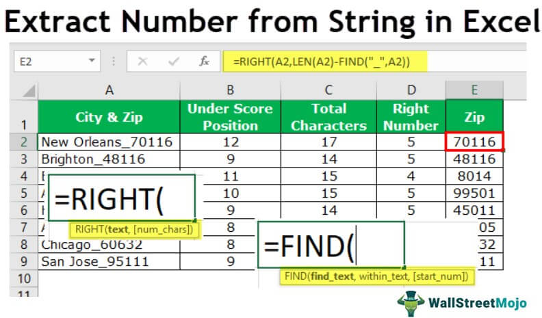
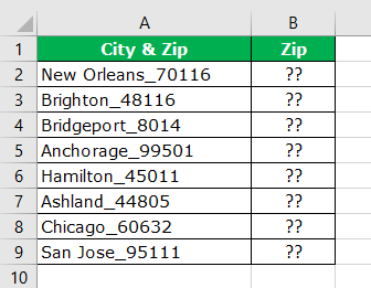
When we get the data, it follows a certain pattern, and having all the numbers at the end of the string is one of the patterns.
- For example, the city with its zip code below is a sample of the same.

- We have the city name and zip code in the above example. In this case, we know we have to extract the zip code from the right-hand side of the string. But, we do not know exactly how many digits we need from the right-hand side of the string.
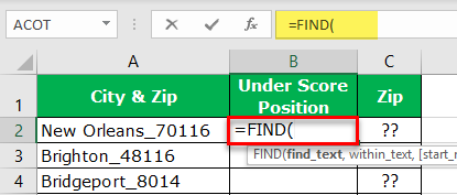
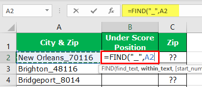
Before the numerical value starts, one of the common things is the underscore (_) character. So first, we need to identify the position of the underscore character. We can do it by using the FIND method. So, apply the FIND function in excel.

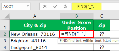
- What text do we need to find in the find_text argument? In this example, we need to find the position of the underscore, so enter the underscore in double quotes.

- The within_text is in which text we need to find the mentioned text, so select cell reference.

- The last argument is not required, so leave it as of now.

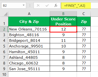
- So, we have got positions of underscore character for each cell. Next, we need to identify how many characters we have in the entire text. So, we must apply the LEN function in Excel to get the total length of the text value.

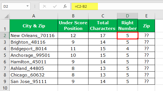
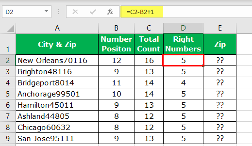
- Now, we have total characters and positions of underscore before the numerical value. Therefore, to supply the number of characters needed for the RIGHT function, we must minus the Total Characters with Underscore Position.

- Now, apply the RIGHT function in cell E2.

- So, like this, we can get the numbers from the right-hand side when we have a common letter before the number starts in the string value. Instead of having so many helper columns, we can apply the formula in a single cell.


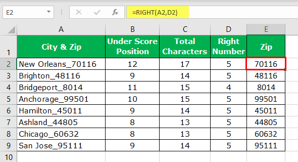
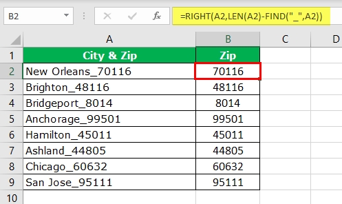
=RIGHT(A2,LEN(A2)-FIND(“_”,A2))
It will eliminate all the supporting columns and reduce the time drastically.
#2 – Extract Numbers From Right Side but Without Special Characters
Assume we have the same data, but this time we do not have any special character before the numerical value.
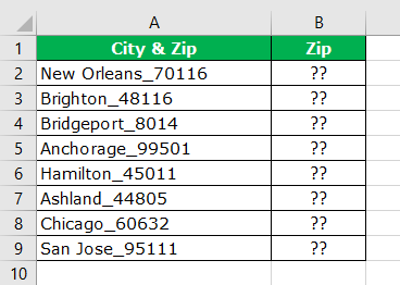
We have found a special character position in the previous example, but we do not have that luxury here. So, the formula below will find the “Numerical Position.”
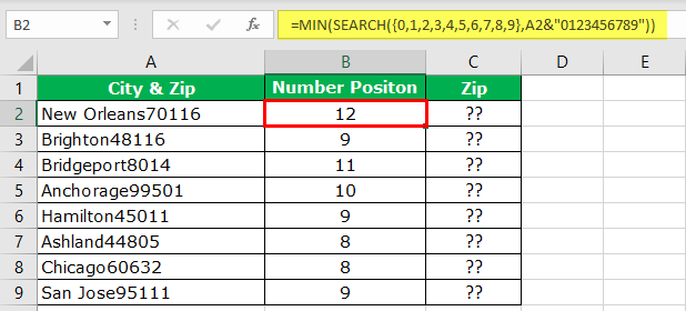
Please do not turn off your computer by looking at the formula. We will decode this for you.
For the SEARCH function in excelSearch function gives the position of a substring in a given string when we give a parameter of the position to search from. As a result, this formula requires three arguments. The first is the substring, the second is the string itself, and the last is the position to start the search.read more, we have supplied all the possible starting numbers of numbers, so the formula looks for the position of the numerical value. Since we have provided all the possible numbers to the array, the resulting arrays should contain the same numbers. Then, the MIN function in excelIn Excel, the MIN function is categorized as a statistical function. It finds and returns the minimum value from a given set of data/array.read more returns the smallest number among the two, so the formula reads below.
=MIN(SEARCH({0,1,2,3,4,5,6,7,8,9},A2&”0123456789″))
So, now we have the “Numerical Position.” But, first, let us find the total number of characters in the cell.
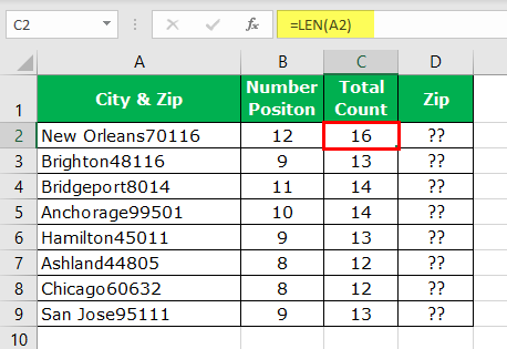
Consequently, it will return the total number of characters in the supplied cell value. Now, the “LEN” – position of the numerical value will return the number of characters required from the right side, so apply the formula to get the number of characters.
Now, we must apply the RIGHT function in excelRight function is a text function which gives the number of characters from the end from the string which is from right to left. For example, if we use this function as =RIGHT ( “ANAND”,2) this will give us ND as the result.read more to get only the numerical part from the string.
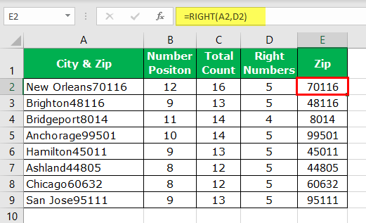
Let us combine the formula in a single cell to avoid multiple helper columns.
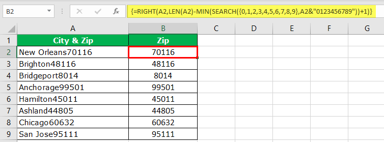
{=RIGHT(A2,LEN(A2)-MIN(SEARCH({0,1,2,3,4,5,6,7,8,9},A2&”0123456789″))+1)}
#3 – Extract Number From Any Position in Excel
We have seen from the RIGHT side extraction. But this is not the case with all the scenarios, so now we will see how to extract numbers from any string position in Excel.
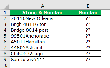
For this, we need to employ various functions of Excel. Below is the formula to extract the numbers from any string position.
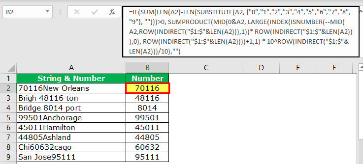
=IF(SUM(LEN(A2)-LEN(SUBSTITUTE(A2, {“0″,”1″,”2″,”3″,”4″,”5″,”6″,”7″,”8″,”9”}, “”)))>0, SUMPRODUCT(MID(0&A2, LARGE(INDEX(ISNUMBER(–MID(A2,ROW(INDIRECT(“$1:$”&LEN(A2))),1))* ROW(INDIRECT(“$1:$”&LEN(A2))),0), ROW(INDIRECT(“$1:$”&LEN(A2))))+1,1) * 10^ROW(INDIRECT(“$1:$”&LEN(A2)))/10),””)
Recommended Articles
This article is a guide to Extract Number From String in Excel. We discussed the top 3 easy methods, step-by-step examples, and a downloadable Excel template. You may learn more about Excel from the following articles: –
- MID Function in Excel
- REPLACE Function in Excel
- Substring in Excel
- VBA String Functions
Watch Video – How to Extract Numbers from text String in Excel (Using Formula and VBA)
There is no inbuilt function in Excel to extract the numbers from a string in a cell (or vice versa – remove the numeric part and extract the text part from an alphanumeric string).
However, this can be done using a cocktail of Excel functions or some simple VBA code.
Let me first show you what I am talking about.
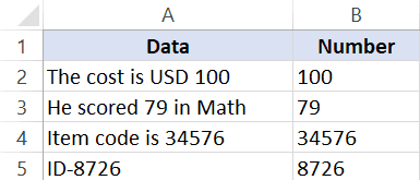
Suppose you have a data set as shown below and you want to extract the numbers from the string (as shown below):
The method you choose will also depend on the version of Excel you’re using:
- For versions prior to Excel 2016, you need to use slightly longer formulas
- For Excel 2016, you can use the newly introduced TEXTJOIN function
- VBA method can be used in all the versions of Excel
Click here to download the example file
Extract Numbers from String in Excel (Formula for Excel 2016)
This formula will work only in Excel 2016 as it uses the newly introduced TEXTJOIN function.
Also, this formula can extract the numbers that are at the beginning, end or middle of the text string.
Note that the TEXTJOIN formula covered in this section would give you all the numeric characters together. For example, if the text is “The price of 10 tickets is USD 200”, it will give you 10200 as the result.
Suppose you have the dataset as shown below and you want to extract the numbers from the strings in each cell:
Below is the formula that will give you numeric part from a string in Excel.
=TEXTJOIN("",TRUE,IFERROR((MID(A2,ROW(INDIRECT("1:"&LEN(A2))),1)*1),""))
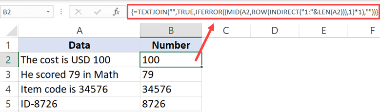
This is an array formula, so you need to use ‘Control + Shift + Enter‘ instead of using Enter.
In case there are no numbers in the text string, this formula would return a blank (empty string).
How does this formula work?
Let me break this formula and try and explain how it works:
- ROW(INDIRECT(“1:”&LEN(A2))) – this part of the formula would give a series of numbers starting from one. The LEN function in the formula returns the total number of characters in the string. In the case of “The cost is USD 100”, it will return 19. The formulas would thus become ROW(INDIRECT(“1:19”). The ROW function will then return a series of numbers – {1;2;3;4;5;6;7;8;9;10;11;12;13;14;15;16;17;18;19}
- (MID(A2,ROW(INDIRECT(“1:”&LEN(A2))),1)*1) – This part of the formula would return an array of #VALUE! errors or numbers based on the string. All the text characters in the string become #VALUE! errors and all numerical values stay as-is. This happens as we have multiplied the MID function with 1.
- IFERROR((MID(A2,ROW(INDIRECT(“1:”&LEN(A2))),1)*1),””) – When IFERROR function is used, it would remove all the #VALUE! errors and only the numbers would remain. The output of this part would look like this – {“”;””;””;””;””;””;””;””;””;””;””;””;””;””;””;””;1;0;0}
- =TEXTJOIN(“”,TRUE,IFERROR((MID(A2,ROW(INDIRECT(“1:”&LEN(A2))),1)*1),””)) – The TEXTJOIN function now simply combines the string characters that remains (which are the numbers only) and ignores the empty string.
Pro Tip: If you want to check the output of a part of the formula, select the cell, press F2 to get into the edit mode, select the part of the formula for which you want the output and press F9. You will instantly see the result. And then remember to either press Control + Z or hit the Escape key. DO NOT hit the enter key.
Download the Example File

You can also use the same logic to extract the text part from an alphanumeric string. Below is the formula that would get the text part from the string:
=TEXTJOIN("",TRUE,IF(ISERROR(MID(A2,ROW(INDIRECT("1:"&LEN(A2))),1)*1),MID(A2,ROW(INDIRECT("1:"&LEN(A2))),1),""))
A minor change in this formula is that IF function is used to check if the array we get from MID function are errors or not. If it’s an error, it keeps the value else it replaces it with a blank.
Then TEXTJOIN is used to combine all the text characters.
Caution: While this formula works great, it uses a volatile function (the INDIRECT function). This means that in case you use this with a huge dataset, it may take some time to give you the results. It’s best to create a backup before you use this formula in Excel.
Extract Numbers from String in Excel (for Excel 2013/2010/2007)
If you have Excel 2013. 2010. or 2007, you can not use the TEXTJOIN formula, so you will have to use a complicated formula to get this done.
Suppose you have a dataset as shown below and you want to extract all the numbers in the string in each cell.
The below formula will get this done:
=IF(SUM(LEN(A2)-LEN(SUBSTITUTE(A2, {"0","1","2","3","4","5","6","7","8","9"}, "")))>0, SUMPRODUCT(MID(0&A2, LARGE(INDEX(ISNUMBER(--MID(A2,ROW(INDIRECT("$1:$"&LEN(A2))),1))* ROW(INDIRECT("$1:$"&LEN(A2))),0), ROW(INDIRECT("$1:$"&LEN(A2))))+1,1) * 10^ROW(INDIRECT("$1:$"&LEN(A2)))/10),"")
In case there is no number in the text string, this formula would return blank (empty string).
Although this is an array formula, you don’t need to use ‘Control-Shift-Enter’ to use this. A simple enter works for this formula.
Credit to this formula goes to the amazing Mr. Excel forum.
Again, this formula will extract all the numbers in the string no matter the position. For example, if the text is “The price of 10 tickets is USD 200”, it will give you 10200 as the result.
Caution: While this formula works great, it uses a volatile function (the INDIRECT function). This means that in case you use this with a huge dataset, it may take some time to give you the results. It’s best to create a backup before you use this formula in Excel.
Separate Text and Numbers in Excel Using VBA
If separating text and numbers (or extracting numbers from the text) is something you have to often, you can also use the VBA method.
All you need to do is use a simple VBA code to create a custom User Defined Function (UDF) in Excel, and then instead of using long and complicated formulas, use that VBA formula.
Let me show you how to create two formulas in VBA – one to extract numbers and one to extract text from a string.
Extract Numbers from String in Excel (using VBA)
In this part, I will show you how to create the custom function to get only the numeric part from a string.
Below is the VBA code we will use to create this custom function:
Function GetNumeric(CellRef As String)
Dim StringLength As Integer
StringLength = Len(CellRef)
For i = 1 To StringLength
If IsNumeric(Mid(CellRef, i, 1)) Then Result = Result & Mid(CellRef, i, 1)
Next i
GetNumeric = Result
End Function
Here are the steps to create this function and then use it in the worksheet:
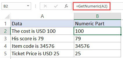
Now, you will be able to use the GetText function in the worksheet. Since we have done all the heavy lifting in the code itself, all you need to do is use the formula =GetNumeric(A2).
This will instantly give you only the numeric part of the string.
Note that since the workbook now has VBA code in it, you need to save it with .xls or .xlsm extension.
Download the Example File
In case you have to use this formula often, you can also save this to your Personal Macro Workbook. This will allow you to use this custom formula in any of the Excel workbooks that you work with.
Extract Text from a String in Excel (using VBA)
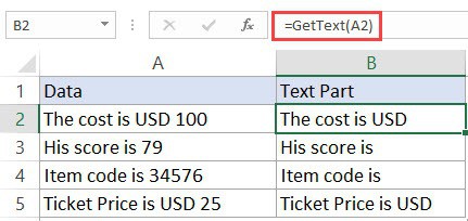
In this part, I will show you how to create the custom function to get only the text part from a string.
Below is the VBA code we will use to create this custom function:
Function GetText(CellRef As String)
Dim StringLength As Integer
StringLength = Len(CellRef)
For i = 1 To StringLength
If Not (IsNumeric(Mid(CellRef, i, 1))) Then Result = Result & Mid(CellRef, i, 1)
Next i
GetText = Result
End Function
Here are the steps to create this function and then use it in the worksheet:
Now, you will be able to use the GetNumeric function in the worksheet. Since we have done all the heavy lifting in the code itself, all you need to do is use the formula =GetText(A2).
This will instantly give you only the numeric part of the string.
Note that since the workbook now has VBA code in it, you need to save it with .xls or .xlsm extension.
In case you have to use this formula often, you can also save this to your Personal Macro Workbook. This will allow you to use this custom formula in any of the Excel workbooks that you work with.
In case you’re using Excel 2013 or prior versions and don’t have
You May Also Like the Following Excel Tutorials:
- CONCATENATE Excel Ranges (with and without separator).
- A Beginner’s Guide to Using For Next Loop in Excel VBA.
- Using Text to Columns in Excel.
- How to Extract a Substring in Excel (Using TEXT Formulas).
- Excel Macro Examples for VBA Beginners.
- Separate Text and Numbers in Excel
Extracting numbers from a list of cells with mixed text is a common data cleaning task.
Unfortunately, there is no direct menu or function created in Excel to help us accomplish this.
In this tutorial we will look at three cases where you might have a list of mixed text, from which you might want to extract numbers:
- When the number is always at the end of the text
- When the number is always at the beginning of the text
- When the number can be anywhere in the text
We will look at three different formulas that can be used to extract the numbers in each case.
At the end of the tutorial, we will also take a look at some VBA code that you can use to accomplish the same.
Brace yourself, this might get a little complex!
Extracting a Number from Mixed Text when Number is Always at the End of the Text
Consider the following example:

Here, each cell has a mix of text and numbers, with the number always appearing at the end of the text. In such cases, we will need to use a combination of nested Excel functions to extract the numbers.
The functions we will use are:
- FIND – This function searches for a character or string in another string and returns its position.
- MIN – This function returns the smallest value in a list.
- LEFT – This function extracts a given number of characters from the left side of a string.
- SUBSTITUTE – This function replaces a particular substring of a given text with another substring.
- IFERROR – This function returns an alternative result or formula if it finds an error in a given formula.
Essentially, we will be using the above functions altogether to perform the following sequence of tasks:
- Find the position of the first numeric value in the given cell
- Extract and remove the text part of the given cell (by removing everything to the left of the first numeric digit)
The formula that we will use to extract the numbers from cell A2 is as follows:
=SUBSTITUTE(A2,LEFT(A2,MIN(IFERROR(FIND({0,1,2,3,4,5,6,7,8,9},A2),""))-1),"")
Let us break down this formula to understand it better. We will go from the inner functions to the outer functions:
- FIND({0,1,2,3,4,5,6,7,8,9},A2)
This function tries to find the positions of all the numbers (0-9) in the cell A2. Thus it returns an arrayformula:
{#VALUE!,#VALUE!,#VALUE!,#VALUE!,#VALUE!,#VALUE!,9,7,8,#VALUE!}
It returns a #VALUE! error for all digits except the 7th, 8th, and 9th digits because it was not able to find these numbers (0,1,2,3,4,5,9) in cell A2. It simply returns the positions of numbers 6,7 and 8 which are the 9th, 7th, and 8th characters respectively in A2.
- IFERROR(FIND({0,1,2,3,4,5,6,7,8,9},A2),””)
Next, the IFERROR function replaces all the error elements of the array with a blank (“”). As such it returns the arrayformula:
{“”,””,””,””,””,””,9,7,8,””}
- MIN(IFERROR(FIND({0,1,2,3,4,5,6,7,8,9},A2),””))
After this the MIN function finds the array element with least value. This is basically the position of the first numeric character in A2. The function now returns the value 7.
- LEFT(A2,MIN(IFERROR(FIND({0,1,2,3,4,5,6,7,8,9},A2),””))-1)
At this point we want to extract all text characters from A2 (so that we can remove them). So we want the LEFT function to extract all the characters starting backwards from the 7-1= 6th character. Thus we use the above formula. The result we get at this point is “arnold”. Notice we subtracted 1 from the second parameter of the LEFT function.
- SUBSTITUTE(A2,LEFT(A2,MIN(IFERROR(FIND({0,1,2,3,4,5,6,7,8,9},A2),””))-1),””)
Now all that’s left to do is remove the string obtained, by replacing it with a blank. This can be easily achieved by using the SUBSTITUTE function: We finally get the numeric characters in the mixed text, which is “786”.
Once you are done entering the formula, make sure you press CTRL+SHIFT+Enter, instead of just the return key. This is because the formula involves arrays.
In a nutshell, here’s what’s happening when you break down the formula:
=SUBSTITUTE(A2,LEFT(A2,MIN(IFERROR(FIND({0,1,2,3,4,5,6,7,8,9},A2),””))-1),””)
=SUBSTITUTE(A2,LEFT(A2,MIN(IFERROR({{#VALUE!,#VALUE!,#VALUE!,#VALUE!,#VALUE!,#VALUE!,9,7,8,#VALUE!}),””))-1),””)
=SUBSTITUTE(A2,LEFT(A2,MIN({“”,””,””,””,””,””,9,7,8,””}))-1),””)
=SUBSTITUTE(A2,”arnold”,””)
=786
When you drag the formula down to the rest of the cells, here’s the result you get:

Also read: How to Generate Random Letters in Excel?
Extracting a Number from Mixed Text when Number is Always at the Beginning of the Text
Now let us consider the case where the numbers are always at the beginning of the Text.
Consider the following example:

Here, each cell has a mix of text and numbers, with the number always appearing at the beginning of the text. In such cases, we will again need to use a combination of nested Excel functions to extract the numbers.
In addition to the functions we used in the previous formula, we are going to use two additional functions. These are:
- MAX – This function returns the largest value in a list
- RIGHT – This function extracts a given number of characters from the right side of a string
- LEN – This function finds the length of (number of characters in) a given string.
Essentially, we will be using these functions altogether to perform the following sequence of tasks:
- Find the position of the last numeric value in the given cell
- Extract and remove the text part of the given cell (by removing everything to the right of the last numeric digit)
The formula that we will use to extract the numbers from cell A2 is as follows:
=SUBSTITUTE(A2,RIGHT(A2,LEN(A2)-MAX(IFERROR(FIND({0,1,2,3,4,5,6,7,8,9},A2),""))),"")
Let us break down this formula to understand it better. We will go from the inner functions to the outer functions:
- FIND({0,1,2,3,4,5,6,7,8,9},A2)
This function tries to find the positions of all the numbers (0-9) in the cell A2. Thus it returns an arrayformula:
{#VALUE!,#VALUE!,1,#VALUE!,#VALUE!,2,#VALUE!,#VALUE!,#VALUE!,#VALUE!}
It returns a #VALUE! error for all digits except the 3rd and 6th digits because it was not able to find these numbers (0,1,3,4,6,7,8,9) in cell A2. It simply returns the positions of numbers 2 and 5 which are the 1st and 2nd characters respectively in A2.
- IFERROR(FIND({0,1,2,3,4,5,6,7,8,9},A2),””)
Next, the IFERROR function replaces all the error elements of the array with a blank. As such it returns the array formula:
{“”,””,1,””,””,2,””,””,””,””}
- MAX(IFERROR(FIND({0,1,2,3,4,5,6,7,8,9},A2),””))
After this the MAX function finds the array element with the highest value. This is basically the position of the last numeric character in A2. The function now returns the value 2.
- LEN(A2)-MAX(IFERROR(FIND({0,1,2,3,4,5,6,7,8,9},A2),””))
At this point we want to extract all text characters from A2 (so that we can remove them). We need to specify how many characters we want to remove. This is obtained by computing the length of the string in A2 minus the position of the last numeric value.Thus we will get the value 8-2 = “6”.
- RIGHT(A2,LEN(A2)-MAX(IFERROR(FIND({0,1,2,3,4,5,6,7,8,9},A2),””)))
We can now use the RIGHT function to extract 6 characters starting from the 2nd character onwards. The result we get at this point is “arnold”.
- SUBSTITUTE(A2,RIGHT(A2,LEN(A2)-MAX(IFERROR(FIND({0,1,2,3,4,5,6,7,8,9},A2),””))),””)
Now all that’s left to do is remove this string by replacing it with a blank. This is easily achieved by using the SUBSTITUTE function. We finally get the numeric characters in the mixed text, which is “25”.
Again, once you are done entering the formula, don’t forget to press CTRL+SHIFT+Enter, instead of just the return key.
In a nutshell, here’s what’s happening when you break down the formula:
=SUBSTITUTE(A7,RIGHT(A7,LEN(A7)-MAX(IFERROR(FIND({0,1,2,3,4,5,6,7,8,9},A7),””))),””)
=SUBSTITUTE(A7,RIGHT(A7,LEN(A7)-MAX(IFERROR({#VALUE!,#VALUE!,1,#VALUE!,#VALUE!,2,#VALUE!,#VALUE!,#VALUE!,#VALUE!}
),””))),””)
=SUBSTITUTE(A7,RIGHT(A7,LEN(A7)-MAX({“”,””,1,””,””,2,””,””,””,””}
)),””)
=SUBSTITUTE(A7,RIGHT(A7,LEN(A7)-2),””)
=SUBSTITUTE(A7,RIGHT(A7,8-2),””)
=SUBSTITUTE(A7,”arnold”,””)
=25
When you drag the formula down to the rest of the cells, here’s the result you get:

Extracting a Number from Mixed Text when Number can be Anywhere in the Text
Finally let us consider the case where the numbers can be anywhere in the text, be it the beginning, end or middle part of the text.
Let’s take a look at the following example:

Here, each cell has a mix of text and numbers, where the number appears in any part of the text. In such cases, we will need to use a combination of nested Excel functions to extract the numbers.
Here are the functions that we are going to use this time:
- INDIRECT – This function simply returns a reference to a range of values.
- ROW – This function returns a row number of a reference.
- MID – This function extracts a given number of characters from the middle of a string.
- TEXTJOIN – This function combines text from multiple ranges or strings using a specified delimiter between them.
Note that the formula discussed in this section will work only in Excel version 2016 onwards as it uses the newly introduced TEXTJOIN function. If you are using an older version of Excel, then you may consider using the VBA method instead (discussed in the next section).
In this method, we will essentially be using the above functions altogether to perform the following sequence of tasks:
- Break up the given text into an array of individual characters
- Find out and remove all characters that are not numbers
- Combine the remaining characters into a full number
The formula that we will use to extract the numbers from cell A2 is as follows:
=TEXTJOIN("",TRUE,IFERROR(MID(A2,ROW(INDIRECT("1:"&LEN(A2))),1)*1,""))
Let us break down this formula to understand it better. We will go from the inner functions to the outer functions:
- LEN(A2)
This function finds the length of the string in cell A2. In our case it returns 13.
- INDIRECT(“1:”&LEN(A2))
This function just returns a reference to all the rows from row 1 to row 12.
- ROW(INDIRECT(“1:”&LEN(A2)))
Now this function returns the row numbers of each of these rows. In other words, it simply returns an array of numbers 1 to 12. This function thus returns the array:
{1;2;3;4;5;6;7;8;9;10;11;12;13}
Note: We use the ROW() function instead of simply hard-coding an array of numbers 1 to 12 because we want to be able to customize this formula depending on the size of the string being worked on. This will ensure that the function adjusts itself when copied to another cell. ·
- MID(A2,ROW(INDIRECT(“1:”&LEN(A2))),1)
Next the MID function extracts the character from A2 that corresponds to each position specified in the array. In other words, it returns an array containing each character of the text in A2 as a separate element, as follows:
{“a”;”r”;”n”;”o”;”l”;”d”;”1″;”4″;”3″;”b”;”l”;”u”;”e”}
- IFERROR(MID(A2,ROW(INDIRECT(“1:”&LEN(A2))),1)*1,””)
After this, the IFERROR function replaces all the elements of the array that are non-numeric. This is because it checks if the array element can be multiplied by 1. If the element is a number, it can easily be multiplied to return the same number. But if the element is a non-numeric character, then it cannot be multiplied with 1 and thus returns an error.
The IFERROR function here specifies that if an element gives an error on multiplication, the result returned will be blank. As such it returns the arrayformula:
{“”;””;””;””;””;””;1;4;3;””;””;””;””}
- TEXTJOIN(“”,TRUE,IFERROR(MID(A2,ROW(INDIRECT(“1:”&LEN(A2))),1)*1,””))
Finally, we can simply combine the array elements together using the TEXTJOIN function. The TEXTJOIN function here combines the string characters that remain (which are the numbers only) and ignores the empty string characters. We finally get the numeric characters in the mixed text, which is “143”.
Once you are done entering the formula, don’t forget to press CTRL+SHIFT+Enter, instead of just the return key.
In a nutshell, here’s what’s happening when you break down the formula:
=TEXTJOIN(“”,TRUE,IFERROR(MID(A2,ROW(INDIRECT(“1:”&LEN(A2))),1)*1,””))
=TEXTJOIN(“”,TRUE,IFERROR(MID(A2,ROW(INDIRECT(“1:”&13)),1)*1,””))
=TEXTJOIN(“”,TRUE,IFERROR(MID(A2,{1;2;3;4;5;6;7;8;9;10;11;12;13},1)*1,””))
=TEXTJOIN(“”,TRUE,IFERROR({“a”;”r”;”n”;”o”;”l”;”d”;”1″;”4″;”3″;”b”;”l”;”u”;”e”}
*1,””))
=TEXTJOIN(“”,TRUE,IFERROR(MID(A2,{1;2;3;4;5;6;7;8;9;10;11;12;13},1)*1,””))
=TEXTJOIN(“”,TRUE, {“”;””;””;””;””;””;1;4;3;””;””;””;””})
=143
When you drag the formula down to the rest of the cells, here’s the result you get:

Using VBA to Extract Number from Mixed Text in Excel
The above method works well enough in extracting numbers from anywhere in a mixed text.
However, it requires one to use the TEXTJOIN function, which is not available in older Excel versions (versions before Excel 2016).
If you’re on a version of Excel that does not support TEXTJOIN, then you can, instead, use a snippet of VBA code to get the job done.
If you have never used VBA before, don’t worry. All you need to do is copy the code below into your VBA developer window and run it on your worksheet data.
Here’s the code that you will need to copy:
'Code by Steve Scott from spreadsheetplanet.com
Function ExtractNumbers(CellRef As String)
Dim StringLength As Integer
StringLength = Len(CellRef)
For i = 1 To StringLength
   If (IsNumeric(Mid(CellRef, i, 1))) Then Result = Result & Mid(CellRef, i, 1)
Next i
ExtractNumbers = Result
End Function
The above code creates a user-defined function called ExtractNumbers() that you can use in your worksheet to extract numbers from mixed text in any cell.
To get to your VBA developer window, follow these steps:
- From the Developer tab, select Visual Basic.

- Once your VBA window opens, Click Insert->Module. That’s it, you can now start coding.

Type or copy-paste the above lines of code into the module window. Your code is now ready to run.

Now, whenever you want to extract numbers from a cell, simply type the name of the function, passing the cell reference as a parameter. So to extract numbers from a cell A2, you will simply need to type the function as follows in a cell:
=ExtractNumbers(A2)

Explanation of the Code
Now let us take some time to understand how this code works.
- In this code, we defined a function named ExtractNumbers, that takes the string in the cell we want to work on. We assigned the name CellRef to this string.
Function ExtractNumbers(CellRef As String)
- We created a variable named StringLength, that will hold the length of the string, CellRef.
Dim StringLength As Integer
StringLength = Len(CellRef)
- Next, we loop through each character in the string CellRef and find out if it is a number. We use the function Mid(CellRef, i, 1) to extract a character from the string at each iteration of the loop. We also use the IsNumeric() function to find out if the extracted character is a number. Each extracted numeric character is combined together into a string called Result.
For i = 1 To StringLength
If (IsNumeric(Mid(CellRef, i, 1))) Then Result = Result & Mid(CellRef, i, 1)
Next i
- This Result is then returned by the function.
ExtractNumbers = Result
Note that since the workbook now has VBA code in it, you need to save it with .xls or .xlsm extension.
You can also choose to save this to your Personal Macro Workbook, if you think you will be needing to run this code a lot. This will allow you to run the code on any Excel workbook of yours.
Well, that was a lot!
In this tutorial, we showed you how to extract numbers from mixed text in excel.
We saw three cases where the numbers are situated in different parts of the text. We also showed you how to use VBA to get the task done quickly.
Other Excel articles you may also like:
- How to Extract URL from Hyperlinks in Excel (Using VBA Formula)
- How to Reverse a Text String in Excel (Using Formula & VBA)
- How to Add Text to the Beginning or End of all Cells in Excel
- How to Remove Text after a Specific Character in Excel (3 Easy Methods)
- How to Separate Address in Excel?
- How to Extract Text After Space Character in Excel?
- How to Find the Last Space in Text String in Excel?
- How to Remove Space before Text in Excel