
Excel for Microsoft 365 Excel for the web Excel 2021 Excel 2019 Excel 2016 Excel 2013 Excel 2010 Excel 2007 More…Less
You can refer to the contents of cells in another workbook by creating an external reference formula. An external reference (also called a link) is a reference to a cell or range on a worksheet in another Excel workbook, or a reference to a defined name in another workbook.
-
Open the workbook that will contain the external reference (the destination workbook) and the workbook that contains the data that you want to link to (the source workbook).
-
Select the cell or cells where you want to create the external reference.
-
Type = (equal sign).
If you want to use a function, such as SUM, then type the function name followed by an opening parenthesis. For example, =SUM(.
-
Switch to the source workbook, and then click the worksheet that contains the cells that you want to link.
-
Select the cell or cells that you want to link to and press Enter.
Note: If you select multiple cells, like =[SourceWorkbook.xlsx]Sheet1!$A$1:$A$10, and have a current version of Microsoft 365, then you can simply press ENTER to confirm the formula as a dynamic array formula. Otherwise, the formula must be entered as a legacy array formula by pressing CTRL+SHIFT+ENTER. For more information on array formulas, see Guidelines and examples of array formulas.
-
Excel will return you to the destination workbook and display the values from the source workbook.
-
Note that Excel will return the link with absolute references, so if you want to copy the formula to other cells, you’ll need to remove the dollar ($) signs:
=[SourceWorkbook.xlsx]Sheet1!$A$1
If you close the source workbook, Excel will automatically append the file path to the formula:
=’C:Reports[SourceWorkbook.xlsx]Sheet1′!$A$1
-
Open the workbook that will contain the external reference (the destination workbook) and the workbook that contains the data that you want to link to (the source workbook).
-
Select the cell or cells where you want to create the external reference.
-
Type = (equal sign).
-
Switch to the source workbook, and then click the worksheet that contains the cells that you want to link.
-
Press F3, select the name that you want to link to and press Enter.
Note: If the named range references multiple cells, and you have a current version of Microsoft 365, then you can simply press ENTER to confirm the formula as a dynamic array formula. Otherwise, the formula must be entered as a legacy array formula by pressing CTRL+SHIFT+ENTER. For more information on array formulas, see Guidelines and examples of array formulas.
-
Excel will return you to the destination workbook and display the values from the named range in the source workbook.
-
Open the destination workbook and the source workbook.
-
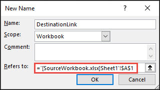
In the destination workbook, Go to Formulas > Defined Names > Define Name.

-
In the New Name dialog box, in the Name box, type a name for the range.
-
In the Refers to box, delete the contents, and then keep the cursor in the box.
If you want the name to use a function, enter the function name, and then position the cursor where you want the external reference. For example, type =SUM(), and then position the cursor between the parentheses.
-
Switch to the source workbook, and then click the worksheet that contains the cells that you want to link.
-
Select the cell or range of cells that you want to link, and click OK.
External references are especially useful when it’s not practical to keep large worksheet models together in the same workbook.
-
Merge data from several workbooks You can link workbooks from several users or departments and then integrate the pertinent data into a summary workbook. That way, when the source workbooks are changed, you won’t have to manually change the summary workbook.
-
Create different views of your data You can enter all of your data into one or more source workbooks, and then create a report workbook that contains external references to only the pertinent data.
-
Streamline large, complex models By breaking down a complicated model into a series of interdependent workbooks, you can work on the model without opening all of its related sheets. Smaller workbooks are easier to change, don’t require as much memory, and are faster to open, save, and calculate.
Formulas with external references to other workbooks are displayed in two ways, depending on whether the source workbook — the one that supplies data to a formula — is open or closed.
When the source is open, the external reference includes the workbook name in square brackets ([ ]), followed by the worksheet name, an exclamation point (!), and the cells that the formula depends on. For example, the following formula adds the cells C10:C25 from the workbook named Budget.xls.
|
External reference |
|---|
|
=SUM([Budget.xlsx]Annual!C10:C25) |
When the source is not open, the external reference includes the entire path.
|
External reference |
|---|
|
=SUM(‘C:Reports[Budget.xlsx]Annual’!C10:C25) |
Note: If the name of the other worksheet or workbook contains spaces or non-alphabetical characters, you must enclose the name (or the path) within single quotation marks as in the example above. Excel will automatically add these for you when you select the source range.
Formulas that link to a defined name in another workbook use the workbook name followed by an exclamation point (!) and the name. For example, the following formula adds the cells in the range named Sales from the workbook named Budget.xlsx.
|
External reference |
|---|
|
=SUM(Budget.xlsx!Sales) |
-
Select the cell or cells where you want to create the external reference.
-
Type = (equal sign).
If you want to use a function, such as SUM, then type the function name followed by an opening parenthesis. For example, =SUM(.
-
Switch to the worksheet that contains the cells that you want to link to.
-
Select the cell or cells that you want to link to and press Enter.
Note: If you select multiple cells (=Sheet1!A1:A10), and have a current version of Microsoft 365, then you can simply press ENTER to confirm the formula as a dynamic array formula. Otherwise, the formula must be entered as a legacy array formula by pressing CTRL+SHIFT+ENTER. For more information on array formulas, see Guidelines and examples of array formulas.
-
Excel will return to the original worksheet and display the values from the source worksheet.
Create an external reference between cells in different workbooks
-
Open the workbook that will contain the external reference (the destination workbook, also called the formula workbook) and the workbook that contains the data that you want to link to (the source workbook, also called the data workbook).
-
In the source workbook, select the cell or cells you want to link.
-
Press Ctrl+C or go to Home > Clipboard > Copy.
-
Switch to the destination workbook, and then click the worksheet where you want the linked data to be placed.
-
Select the cell where you want to place the linked data, then go to Home > Clipboard > Paste > Paste Link.
-
Excel will return the data you copied from the source workbook. If you change it, it will automatically change in the destination workbook when you refresh your browser window.
-
To use the link in a formula, type = in front of the link, choose a function, type (, and then type ) after the link.
Create a link to a worksheet in the same workbook
-
Select the cell or cells where you want to create the external reference.
-
Type = (equal sign).
If you want to use a function, such as SUM, then type the function name followed by an opening parenthesis. For example, =SUM(.
-
Switch to the worksheet that contains the cells that you want to link to.
-
Select the cell or cells that you want to link to and press Enter.
-
Excel will return to the original worksheet and display the values from the source worksheet.
Need more help?
You can always ask an expert in the Excel Tech Community or get support in the Answers community.
See Also
Define and use names in formulas
Find links (external references) in a workbook
Need more help?
What are External Links in Excel?
External links are also known as the external references in Excel. When we use any formula in Excel and refer to any other workbook apart from the workbook with the formula, the new workbook is the external link to the formula. When we give a link or apply a formula from another workbook, it is called an external link.
If our formula reads like the below, it is an external link.
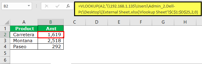
‘C:UsersAdmin_2.Dell-PCDesktop: This is the path to that sheet on the computer.
[External Sheet.xlsx]: This is the “Workbook” name in that path.
Vlookup Sheet: This is the “Worksheet” name in that workbook.
$C$1:$D$25: This is the range in that sheet.
Table of contents
- What are External Links in Excel?
- Types of External Links in Excel
- #1- Links within the Same Worksheet
- #2 – Links from different worksheet but within the same workbook
- #3 – Links from a different workbook
- How to Find, Edit, and Remove External Links in Excel?
- Method #1: Using the Find & Replace Method with Operator Symbol
- Method #2: Using the Find & Replace Method with File Extension
- Method #3: Using Edit Link Option in Excel
- Things to Remember
- Recommended Articles
- Types of External Links in Excel
Types of External Links in Excel
- Links within the same worksheet
- Links from different worksheets but the same workbook
- Links from a different workbook
You can download this External Links Excel Template here – External Links Excel Template
#1- Links within the Same Worksheet
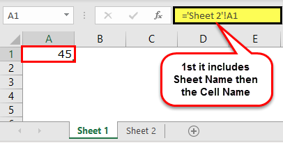
These types of links are within the same worksheet. In a workbook, there are many sheets. This type of link specifies only the cell name.
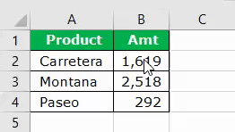
For example, if we are in cell B2 and the formula bar reads A1, whatever happens in the A1 cell will reflect in cell B2.
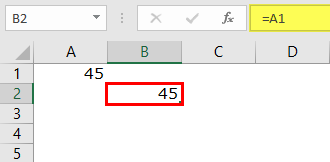
It is just a simple link within the same sheet.
#2 – Links from different worksheets but within the same workbook
These types of links are within the same workbook but from different sheets.
For example, suppose there are two sheets in a workbook, and right now, we are in Sheet1 and giving a link from Sheet2.
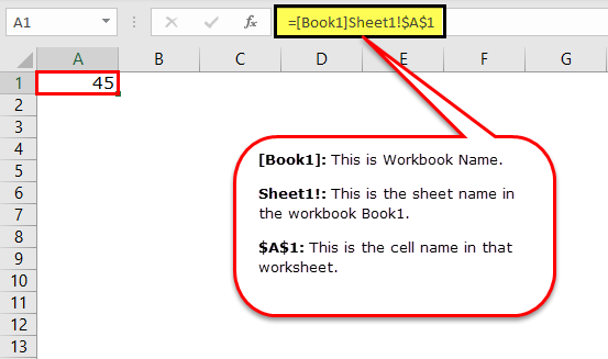
#3 – Links from a different workbook
This type of link is called an external link. It means this is altogether from a different workbook itself.
For example, if we give a link from another workbook called “Book1”, it will first show the workbook name, sheet name, and cell name.
How to Find, Edit, and Remove External Links in Excel?
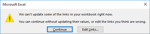
There are multiple ways we can find external links in the Excel workbook. As soon as we open a worksheet, we will get the below dialog box before we get inside the workbook, indicating that this workbook has external links.
Let us explain the methods to find external links in Excel.
Method #1: Using the Find & Replace Method with Operator Symbol
The link must have included its path or URL to the referring workbook if external links exist. The common in all the links is the operator symbol “[. “
Below are the steps to find external links using the “Find & Replace” method.
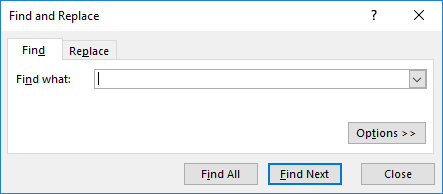
- First, we must select the sheet and press the “Ctrl + F” keys (shortcut to find external links).

- Then, we must insert the symbol “[” and click on “Find All.”
Method #2: Using the Find & Replace Method with File Extension
A cell with external references includes a workbook name and the workbook type.
The common file extensions are .xlsx , .xls , .xlsm , .xlb.
Step 1: First, we must select the sheet and press the “Ctrl + F” (shortcut to find external links).

Step 2: Now, we must insert “.xlsx” and click on “Find All.”
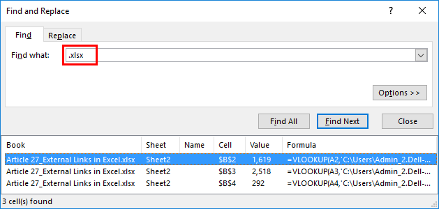
It will show all the external link cells.
Method #3: Using the Edit Link Option in Excel
It is the most direct option we have in Excel. It will highlight only the external link, unlike methods 1 and 2. We can edit the link in Excel, break, or delete and remove external links in this method.
The “Edit Links” option in Excel is available under the “Data” tab.
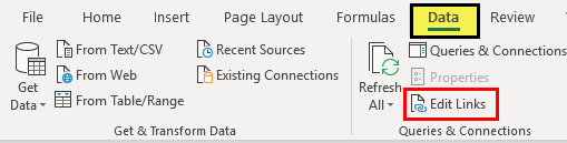
Step 1: We must first select the cells we want to edit, break, or delete the link cells.
Step 2: Now, click on “Edit Links” in Excel. There are several options available here.
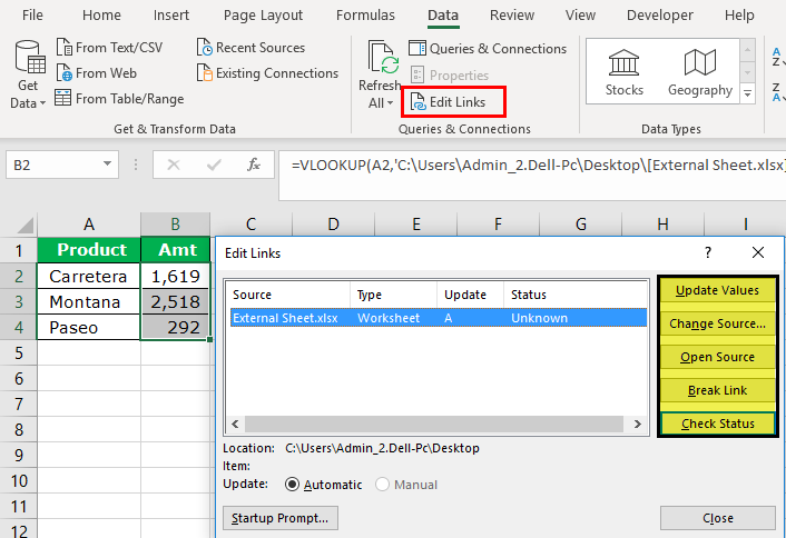
- Update Values: This will update any changed values from the linked sheet.
- Change Source: This will change the source file.
- Open Source: This will open the source file instantly.
- Break Link: This will permanently delete the formula, remove the external link, and retain only the values. Once this is done, we cannot undo it.
- Check Status: This will check the status of the link.
Note: Sometimes, even if there is an external source, these methods would not show anything, but we must manually check graphs, charts, name ranges, data validation, condition formattingConditional formatting is a technique in Excel that allows us to format cells in a worksheet based on certain conditions. It can be found in the styles section of the Home tab.read more, chart title, shapes, or objects.
Things to Remember
- We can find external links by using the VBA codeVBA code refers to a set of instructions written by the user in the Visual Basic Applications programming language on a Visual Basic Editor (VBE) to perform a specific task.read more. We must search on the internet to explore this.
- If the external link is given to shapes, we must look for it manually.
- The external formula links will not show the results in the case of SUMIF Formulas in ExcelThe SUMIF Excel function calculates the sum of a range of cells based on given criteria. The criteria can include dates, numbers, and text. For example, the formula “=SUMIF(B1:B5, “<=12”)” adds the values in the cell range B1:B5, which are less than or equal to 12.
read more, SUMIFS & COUNTIF formulasThe COUNTIF function in Excel counts the number of cells within a range based on pre-defined criteria. It is used to count cells that include dates, numbers, or text. For example, COUNTIF(A1:A10,”Trump”) will count the number of cells within the range A1:A10 that contain the text “Trump”
read more. It will show the values only if the sourced file is opened. - If Excel still shows an external link promptly, we must manually check all the formatting, charts, validation, etc.
- Keeping external links can be helpful in case of auto-updating from the other sheet.
Recommended Articles
This article is a guide to External Links in Excel. Here, we discussed types of links, dealing with external links, finding, editing, and removing external links in Excel, and Excel examples and downloadable Excel templates. You may also look at these useful functions in Excel: –
- Break Links Excel
- Remove Excel Hyperlinks
- VBA Hyperlinks
- Insert Hyperlinks in Excel
Перейти к содержанию
На чтение 2 мин Опубликовано 20.07.2015
- Создание внешней ссылки
- Оповещения
- Редактирование ссылки
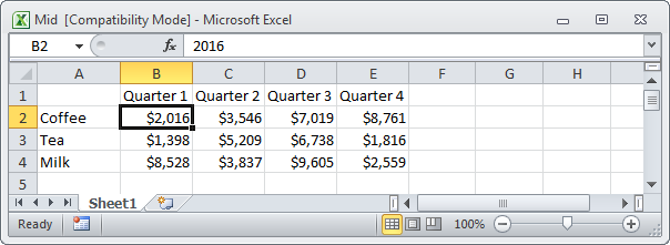
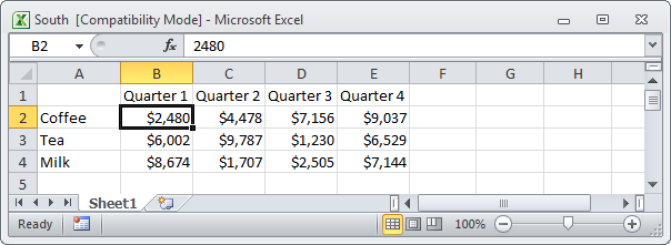
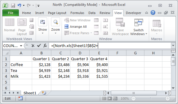
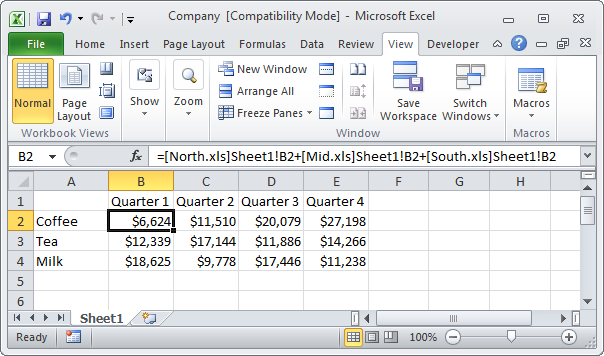
Внешняя ссылка в Excel – это ссылка на ячейку (или диапазон ячеек) в другой книге. На рисунках
ниже вы видите книги из трех отделов (North, Mid и South).

Содержание
- Создание внешней ссылки
- Оповещения
- Редактирование ссылки
Создание внешней ссылки
Чтобы создать внешнюю ссылку, следуйте инструкции ниже:
- Откройте все три документа.
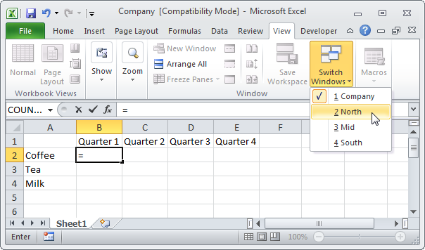
- В книге «Company», выделите ячейку B2 и введите знак равенства «=».
- На вкладке View (Вид) кликните по кнопке Switch Windows (Перейти в другое окно) и выберите «North».
- В книге «North», выделите ячейку B2 и введите «+».
- Повторите шаги 3 и 4 для книг «Mid» и «South».
- Уберите символы «$» в формуле ячейки B2 и скопируйте эту формулу в другие ячейки.Результат:
Оповещения
Закройте все документы. Внесите изменения в книги отделов. Снова закройте все документы. Откройте файл «Company».
- Чтобы обновить все ссылки, кликните по кнопке Enable Content (Включить содержимое).
- Чтобы ссылки не обновлялись, нажмите кнопку X.
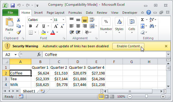
Примечание: Если вы видите другое оповещение, нажмите Update (Обновить) или Don’t Update (Не обновлять).
Редактирование ссылки
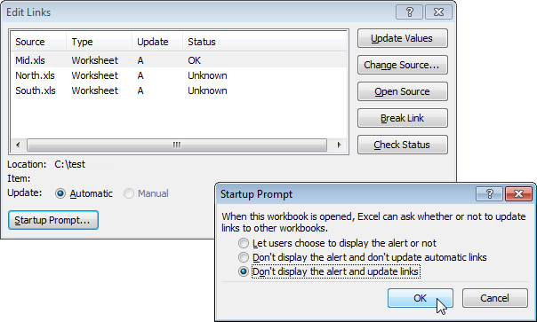
Чтобы открыть диалоговое окно Edit Links (Изменение связей), на вкладке Data (Данные) в разделе Connections group (Подключения) щелкните Edit links symbol (Изменить связи).
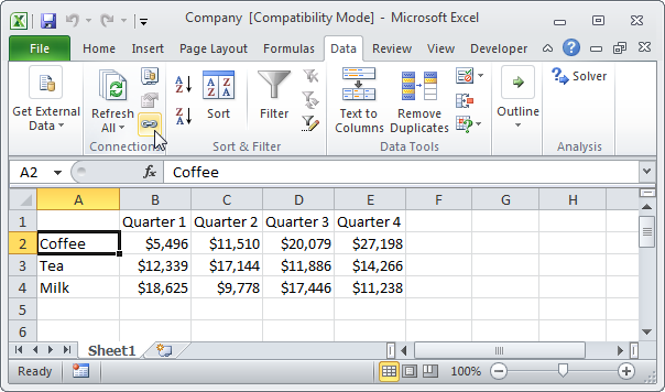
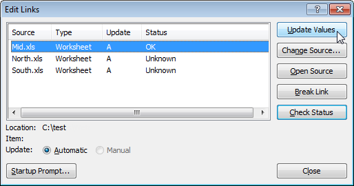
- Если вы не обновили ссылки сразу, можете обновить их здесь. Выберите книгу и нажмите кнопку Update Values (Обновить), чтобы обновить ссылки на эту книгу. Обратите внимание, что Status (Статус) изменяется на ОК.
- Если вы не хотите обновлять ссылки автоматически и не желаете, чтобы отображались уведомления, кликните по кнопке Startup Prompt (Запрос на обновление связей), выберите третий вариант и нажмите ОК.
Оцените качество статьи. Нам важно ваше мнение:
What are External Links or References?
When you create formulas in Excel and refer to a data point in an another workbook, Excel creates a link to that workbook.
So your formula may look like something as shown below:
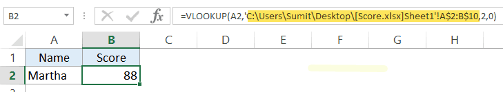
Note that the part highlighted in yellow is the external link (also called external reference). This part of the formula tells Excel to go to this workbook (Score.xlsx) and refer to the specified cell in the workbook.
The benefit of having an external link in your formula is that you can automatically update it when the data in the linked workbook changes.
However, the drawback is that you always need to have that linked workbook available. If you delete the linked workbook file, change its name, or change its folder location, the data would not update.
If you’re working with a workbook that contains externals links and you have to share it with colleagues/clients, it’s better to remove these external links.
However, if you have a lot of formulas, doing this manually can drive you crazy.
How to Find Externals Links and References in Excel
Here are a couple of techniques you can use to quickly find external links in Excel:
- Using Find and Replace.
- Using Edit Links Option.
Let’s see how each of these techniques work.
Find External Links using Find and Replace
Cells with external links contain the name of the workbook to which it links. This would mean that the reference would have the file name with .xlsx/.xls/.xlsm/.xlb extension.
We can use this to find all the external links.
Here are the steps to find external links in Excel using Find and Replace:
This will find and show all the cells that have external links in it.
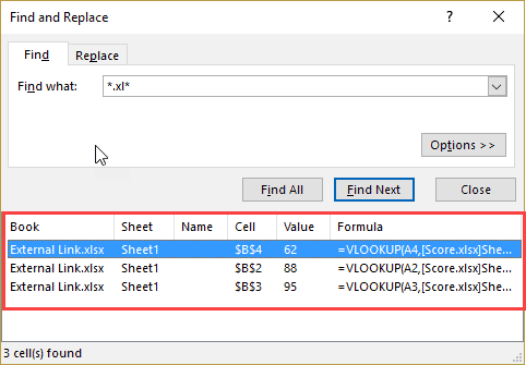
Now you can select all these cells (select the first record, hold the Shift key and then select the last record) and convert the formulas to values.
Find External Links using Edit Links Option
Excel has this inbuilt tool that will find all the externals references.
Here are the steps to find external links using Edit Links Option:
Be aware that once you break the links, you can undo it. As a best practice, create a backup before doing this.
Still Getting the External Links Prompt?
Sometimes, you may find and remove all the external links, but still get a prompt as shown below:

Don’t go crazy and start cursing Excel.
So if you’re getting the update links prompt, also check the following for external links:
- Named Ranges
- Conditional Formatting
- Data Validation
- Shapes
- Chart Titles
Using ‘Find and Replace’ or ‘Edit Links’ as shown above would not identify external links in these above-mentioned features.
Here are the steps to find external links in these places:
- Named Ranges: Go to the Formula tab and click on Name Manager. It will show you all the named ranges in the workbook. You can check the ‘Refers to’ column to spot external references.
- Conditional Formatting: The only way an external link can land up in Conditional Formatting is through the custom formula. Go to the Home tab –> Conditional Formatting –> Manage Rules. In the Conditional Formatting Rules Manager, check the formulas for external links.
- Data Validation: It is possible that the data validation drop down list refers to a named range that in turn has external links. Checking Named Ranges should take care of this issue as well.
- Shapes: If you’re using shapes that are linked to cells, check these for external links. Here is a quick way to go through all the shapes:
- Press the F5 key. It will open the Go to Dialog Box.
- Click on Special.
- In the Go To Special dialog box, select Objects.
- Click OK. This would select all the shapes. Now you can use the Tab key to cycle through these.
- Chart Titles: Select the chart title and check in the formula bar if it refers to an external link.
You can learn more about External Links from these tutorials:
- Finding External Links in Excel – Contextures Blog.
- Finding External Links – Microsoft Excel Support.
There is also an add-in available to find external links in Excel. Click here to learn more and download the add-in.
You May Also Like the Following Excel Tutorials:
- How to Lock Cells in Excel.
- Find and Remove Hyperlinks in Excel.
- Creating Dynamic Hyperlinks.
- Using FIND function in Excel.
- How to Reference Another Sheet or Workbook in Excel
- How to Find Circular Reference in Excel
![]()
Download Article
Step-by-step guide to creating hyperlinks in Excel
![]()
Download Article
- Linking to a New File
- Linking to an Existing File or Webpage
- Linking Within the Document
- Creating an Email Address Hyperlink
- Using the HYPERLINK Function
- Creating a Link to a Workbook on the Web
- Video
- Q&A
- Tips
- Warnings
|
|
|
|
|
|
|
|
|
This wikiHow teaches you how to create a link to a file, folder, webpage, new document, email, or external reference in Microsoft Excel. You can do this on both the Windows and Mac versions of Excel. Creating a hyperlink is easy using Excel’s built-in link tool. Alternatively, you can use the HYPERLINK function to quickly link to a location.
Things You Should Know
- You can link to a new file, existing file, webpage, email, or location in your document.
- Use the HYPERLINK function if you already have the link location.
- Create an external reference link to another workbook to insert a cell value into your workbook.
-
1
Open an Excel document. Double-click the Excel document in which you want to insert a hyperlink.
- You can also open a new document by double-clicking the Excel icon and clicking Blank Workbook.
-
2
Select a cell. This should be a cell into which you want to insert your hyperlink.
Advertisement
-
3
Click Insert. This tab is in the green ribbon at the top of the Excel window. Clicking Insert opens a toolbar directly below the green ribbon.[1]
- If you’re on a Mac, note that there’s an Excel Insert tab and an Insert menu item in your Mac’s menu bar. Select the Excel Insert tab.
-
4
Click Link. It’s toward the right side of the Insert toolbar in the «Links» section. Doing so opens a pop up menu.
-
5
Click Insert Link. It’s at the bottom of the Link pop up menu. This opens the Insert Hyperlink window.
-
6
Click Create New Document. This tab is on the left side of the pop-up window, under “Link to:”.
- This option is not available on some versions of Excel. You’ll need to create the new document before making the hyperlink, then use the Existing File or Web Page option.
-
7
Enter the hyperlink’s text. Type the text that you want to see displayed into the «Text to display» field. This is the box above the “Name of new document” field.
-
8
Type in a name for the new document. Do so in the «Name of new document» field.
-
9
Click OK. It’s at the bottom of the window. By default, this will create and open a new spreadsheet document, then create a link to it in the cell that you selected in the other spreadsheet document.
- You can also select the «Edit the new document later» option before clicking OK to create the spreadsheet and the link without opening the spreadsheet.
- If something goes wrong with the hyperlink, see our guide for fixing a hyperlink in Excel.


Advertisement
-
1
Open an Excel document. Double-click the Excel document in which you want to insert a hyperlink.
- You can also open a new document by double-clicking the Excel icon and then clicking Blank Workbook.
- Hyperlinks are a great way to organize and connect information across multiple Excel documents. You can also easily create hyperlinks in PowerPoint if you have a presentation coming up.
-
2
Select a cell. This should be a cell into which you want to insert your hyperlink.
-
3
Click Insert. This tab is in the green ribbon at the top of the Excel window. Clicking Insert opens a toolbar directly below the green ribbon.
- If you’re on a Mac, note that there’s an Excel Insert tab and an Insert menu item in your Mac’s menu bar. Select the Excel Insert tab.
-
4
Click Link. It’s toward the right side of the Insert toolbar in the «Links» section. Doing so opens a pop up menu.
-
5
Click Insert Link. It’s at the bottom of the Link pop up menu. This opens the Insert Hyperlink window.
-
6
Click the Existing File or Web Page. It’s on the left side of the window.
-
7
Enter the hyperlink’s text. Type the text that you want to see displayed into the «Text to display» field.
- If you don’t do this, your hyperlink’s text will just be the folder path to the linked item.
-
8
Select a destination. You can choose a file location on your computer, enter an address of a file or web page, or browse the internet. Here are the destination options:
- Current Folder — Search for files in your Documents or Desktop folder.
- Browsed Pages — Search through recently viewed web pages.
- Recent Files — Search through recently opened Excel files.
- Type in the location and name of a web page or file into the “Address” field. For example, this could be a URL to a website.
- Click the Browse the Web button (a globe behind a magnifying glass). Go to the web page you’re linking to, then go back to Excel. Don’t close your browser!
-
9
Select a file or webpage. Click the file, folder, or web address to which you want to link. A path to the folder will appear in the «Address» text box at the bottom of the window.
-
10
Click OK. It’s at the bottom of the page. Doing so creates your hyperlink in your specified cell.
- Note that if you move the item to which you linked, the hyperlink will no longer work.


Advertisement
-
1
Open an Excel document. Double-click the Excel document in which you want to insert a hyperlink. This method links to a cell or sheet in your workbook. For example, if you’re tracking your bills in Excel, you can link to a summary sheet from your data sheet.
- You can also open a new document by double-clicking the Excel icon and then clicking Blank Workbook.
-
2
Select a cell. This should be a cell into which you want to insert your hyperlink.
-
3
Click Insert. This tab is in the green ribbon at the top of the Excel window. Clicking Insert opens a toolbar directly below the green ribbon.
- If you’re on a Mac, note that there’s an Excel Insert tab and an Insert menu item in your Mac’s menu bar. Select the Excel Insert tab.
-
4
Click Link. It’s toward the right side of the Insert toolbar in the «Links» section. Doing so opens a pop up menu.
-
5
Click Insert Link. It’s at the bottom of the Link pop up menu. This opens the Insert Hyperlink window.
-
6
Click the Place in This Document. It’s on the left side of the window.
-
7
Select a location in the Excel document. You have two options for selecting a location:
- Under “Type the cell reference,” type in the cell you want to link to.
- Alternatively, under “Or select a place in this document,” click a sheet name or defined name.
-
8
Enter the hyperlink’s text. Type the text that you want to see displayed into the «Text to display» field.
- If you don’t do this, your hyperlink’s text will just be the linked cell’s name.
-
9
Click OK. This will create your link in the selected cell. If you click the hyperlink, Excel will automatically highlight the linked cell or take you to the sheet you selected.
- For general Excel tips, see our intro guide to Excel.


Advertisement
-
1
Open an Excel document. Double-click the Excel document in which you want to insert a hyperlink.
- You can also open a new document by double-clicking the Excel icon and then clicking Blank Workbook.
-
2
Select a cell. This should be a cell into which you want to insert your hyperlink.
-
3
Click Insert. This tab is in the green ribbon at the top of the Excel window. Clicking Insert opens a toolbar directly below the green ribbon.
- If you’re on a Mac, note that there’s an Excel Insert tab and an Insert menu item in your Mac’s menu bar. Select the Excel Insert tab.
-
4
Click Link. It’s toward the right side of the Insert toolbar in the «Links» section. Doing so opens a pop up menu.
-
5
Click Insert Link. It’s at the bottom of the Link pop up menu. This opens the Insert Hyperlink window.
-
6
Click E-mail Address. It’s on the left side of the window.
-
7
Enter the hyperlink’s text. Type the text that you want to see displayed into the «Text to display» field.
- If you don’t change the hyperlink’s text, the email address will display as itself.
-
8
Enter the email address. Type the email address that you want to hyperlink into the «E-mail address» field.
- You can also add a prewritten subject to the «Subject» field, which will cause the hyperlinked email to open a new email message with the subject already filled in.
-
9
Click OK. This button is at the bottom of the window.
- Clicking this email link will automatically open an installed email program with a new email to the specified address.


Advertisement
-
1
Open an Excel document. Double-click the Excel document in which you want to insert a hyperlink.
- You can also open a new document by double-clicking the Excel icon and then clicking Blank Workbook.
-
2
Select a cell. This should be a cell into which you want to insert your hyperlink.
-
3
Type =HYPERLINK(). This function creates a hyperlink to a document on the Internet, an intranet, or a server. This function has two parameters:[2]
- HYPERLINK(link_location,friendly_name)
- link_location is where you type in the path to the file and the file name.
- friendly_name is the text shown for the hyperlink in your Excel spreadsheet. This parameter is optional.
-
4
Add the link location and friendly name. To do so:
- In the parenthesis of the HYPERLINK function, type the file path and file name for the document you want to link to.
- Add a comma (,).
- Type the name you want to appear for the hyperlink.
-
5
Press ↵ Enter. This will confirm the HYPERLINK formula and create the hyperlink in the selected cell. Clicking the link will open the specified file.


Advertisement
-
1
Open an Excel document. Double-click the Excel document in which you want to insert a hyperlink.
- You can also open a new document by double-clicking the Excel icon and then clicking Blank Workbook.
-
2
Open the workbook you want to link to. This can be referred to as the source workbook. This method creates an external reference link to a workbook on the Internet or your intranet.
-
3
Select the cell you want to link to in the source workbook. This will place a green box around the cell.
-
4
Copy the cell. You’ll need to copy the cell to reference it in your workbook. To copy it:
- Go to the Home tab.
- Click Copy in the “Clipboard” section. This button has an icon of two pieces of paper.
-
5
Go to your workbook. This is the workbook that you want to place the external reference link in.
-
6
Select the cell you want to place the link in. You can place the link in any sheet of your workbook.
-
7
Click the Home tab. This will open the Home toolbar.
-
8
Click the Paste drop down button. This is the button below the clipboard with a down arrow. This opens the Paste drop down menu.
-
9
Click the Paste Link button. This is two chains linked together in front of a clipboard in the Paste drop down menu. The value of the external reference will appear in the cell you selected.
- To see the external reference location, select the cell with the external reference. Then, check the Formula Bar for the location.


Advertisement
Add New Question
-
Question
How do I put a hyperlink in a text box?

Right-click on the cell into which you wish to insert the link. Choose ‘Link’ on the menu which pops up, then insert the URL at the bottom of the little Link Setup Window.
-
Question
My Excel chart hyperlinks work on my computer, but not on the computers of folks I send the chart to. Why?
MS Office applications routinely disable links and other potentially harmful content whenever you open a file created on another PC or downloaded from the Internet. A warning message is displayed at the top of the document. The user then has the choice to trust the source of the document, which enables all content, or to view it in «Compatibility Mode,» with potentially harmful content disabled.
-
Question
The hyperlink option in the drop down menu is shaded and I can’t click on it. What should I do?
Highlight the text you want to add a hyperlink to, then click hyperlink.
Ask a Question
200 characters left
Include your email address to get a message when this question is answered.
Submit
Advertisement
Video
Thanks for submitting a tip for review!
Advertisement
-
If you move a file connected to an Excel spreadsheet by hyperlink to a new location, you will have to edit the hyperlink to include the new file location.
Advertisement
About This Article
Thanks to all authors for creating a page that has been read 486,649 times.