Expand and collapse in excel - Word и Excel - помощь в работе с программами

Excel for Microsoft 365 Excel for Microsoft 365 for Mac Excel 2021 Excel 2019 Excel 2016 Excel 2013 More…Less

In a PivotTable or PivotChart, you can expand or collapse to any level of data detail, and even for all levels of detail in one operation. On Windows and the Mac, you can also expand or collapse to a level of detail beyond the next level. For example, starting at a country/region level, you can expand to a city level which expands both the state/province and city level. This can be a time-saving operation when you work with many levels of detail. In addition, you can expand or collapse all members for each field in an Online Analytical Processing (OLAP) data source. You can also see the details that are used to aggregate the value in a value field.

In a PivotTable, do one of the following:

Click the expand or collapse button next to the item that you want to expand or collapse.

Note: If you don’t see the expand or collapse buttons, see the Show or hide the expand and collapse buttons in a PivotTable section in this topic.
Double-click the item that you want to expand or collapse.
Right-click the item, click Expand/Collapse, and then do one of the following:
- To see the details for the current item, click Expand.
- To hide the details for the current item, click Collapse.
- To hide the details for all items in a field, click Collapse Entire Field.
- To see the details for all items in a field, click Expand Entire Field.
- To see a level of detail beyond the next level, click Expand To «<Field name>».
- To hide to a level of detail beyond the next level, click Collapse To «<Field name>».

In a PivotChart, right-click the category label for which you want to show or hide level details, click Expand/Collapse, and then do one of the following:

To see the details for the current item, click Expand.
To hide the details for the current item, click Collapse.
To hide the details for all items in a field, click Collapse Entire Field.
To see the details for all items in a field, click Expand Entire Field.
To see a level of detail beyond the next level, click Expand To «<Field name>».
To hide to a level of detail beyond the next level, click Collapse To «<Field name>».

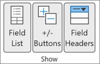
The expand and collapse buttons are displayed by default, but you may have hidden them (for example, when you don’t want them to appear in a printed report). To use these buttons to expand or collapse levels of detail in the report, you must make sure that they are displayed.

In Excel 2016 and Excel 2013: On the Analyze tab, in the Show group, click +/- Buttons to show or hide the expand and collapse buttons.

Note: Expand and collapse buttons are available only for fields that have detail data.

You can show or hide details and disable or enable the corresponding option.

Show value field details

In a PivotTable, do one of the following:
- Right-click a field in the values area of the PivotTable, and then click Show Details.
- Double-click a field in the values area of the PivotTable.
  
  The detail data that the value field is based on is placed on a new worksheet.

Hide value field details

Right-click the sheet tab of the worksheet that contains the value field data, and then click Hide or Delete.

Disable or enable the option to show value field details

Click anywhere in the PivotTable.
On the Options or Analyze tab (depending on the Excel version you are using) on the ribbon, in the PivotTable group, click Options.
In the PivotTable Options dialog box, click the Data tab.
Under PivotTable Data, clear or select the Enable show details check box to disable or enable this option.

Note: This setting is not available for an OLAP data source.

In a PivotTable, do one of the following:

Click the expand or collapse button next to the item that you want to expand or collapse.

Note: If you don’t see the expand or collapse buttons, see the Show or hide the expand and collapse buttons in a PivotTable section in this topic.
Double-click the item that you want to expand or collapse.
Right-click the item, click Expand/Collapse, and then do one of the following:
- To see the details for the current item, click Expand.
- To hide the details for the current item, click Collapse.
- To hide the details for all items in a field, click Collapse Entire Field.
- To see the details for all items in a field, click Expand Entire Field.
- To see a level of detail beyond the next level, click Expand To «<Field name>».
- To hide to a level of detail beyond the next level, click Collapse To «<Field name>».

In a PivotChart, right-click the category label for which you want to show or hide level details, click Expand/Collapse, and then do one of the following:

To see the details for the current item, click Expand.
To hide the details for the current item, click Collapse.
To hide the details for all items in a field, click Collapse Entire Field.
To see the details for all items in a field, click Expand Entire Field.
To see a level of detail beyond the next level, click Expand To «<Field name>».
To hide to a level of detail beyond the next level, click Collapse To «<Field name>».

In Excel 2016 and Excel 2013: On the Analyze tab, in the Show group, click +/- Buttons to show or hide the expand and collapse buttons.

Note: Expand and collapse buttons are available only for fields that have detail data.

You can show or hide details and disable or enable the corresponding option.

Show value field details

In a PivotTable, do one of the following:
- Right-click a field in the values area of the PivotTable, and then click Show Details.
- Double-click a field in the values area of the PivotTable.
  
  The detail data that the value field is based on is placed on a new worksheet.

Hide value field details

Right-click the sheet tab of the worksheet that contains the value field data, and then click Hide or Delete.

Disable or enable the option to show value field details

Click anywhere in the PivotTable.
On the Options or Analyze tab (depending on the Excel version you are using) on the ribbon, in the PivotTable group, click Options.
In the PivotTable Options dialog box, click the Data tab.
Under PivotTable Data, clear or select the Enable show details check box to disable or enable this option.

Note: This setting is not available for an OLAP data source.

In a PivotTable, do one of the following:

Click the expand or collapse button next to the item that you want to expand or collapse.

Note: If you don’t see the expand or collapse buttons, see the Show or hide the expand and collapse buttons in a PivotTable section in this topic.
Double-click the item that you want to expand or collapse.
Right-click the item, click Expand/Collapse, and then do one of the following:
- To see the details for the current item, click Expand.
- To hide the details for the current item, click Collapse.
- To hide the details for all items in a field, click Collapse Entire Field.
- To see the details for all items in a field, click Expand Entire Field.

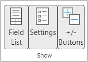
On the PivotTable tab, in the Show group, click +/- Buttons to show or hide the expand and collapse buttons.

Note: Expand and collapse buttons are available only for fields that have detail data.

Showing or hiding details is supported for PivotTables created from a table or range.

Show value field details

In a PivotTable, do one of the following:
- Click anywhere in the PivotTable. On the PivotTable tab, click Show Details.
- Right-click a field in the values area of the PivotTable, and then click Show Details.
- Double-click a field in the values area of the PivotTable.
  
  The detail data that the value field is based on is placed on a new worksheet.

Hide value field details

Right-click the sheet tab of the worksheet that contains the value field data, and then click Hide or Delete.

Need more help?

You can always ask an expert in the Excel Tech Community or get support in the Answers community.

How do you expand and collapse multiple columns in Excel?

About This Article

Click the Data tab.
Click Group.
Select Columns and click OK.
Click – to collapse.
Click + to uncollapse.

What is the shortcut to expand all collapsed rows in Excel?

Press the “Ctrl-Shift-(” keys together to expand all hidden rows in your Excel spreadsheet.

How do you make Excel cells expand to fit text automatically?

Wrap text automatically
On the Home tab, in the Alignment group, click Wrap Text. (On Excel for desktop, you can also select the cell, and then press Alt + H + W.) Notes: Data in the cell wraps to fit the column width, so if you change the column width, data wrapping adjusts automatically.

How do you expand columns in Excel?

Resize columns

Select a column or a range of columns.
On the Home tab, in the Cells group, select Format > Column Width.
Type the column width and select OK.

How does a Vlookup work?

The VLOOKUP function performs a vertical lookup by searching for a value in the first column of a table and returning the value in the same row in the index_number position. The VLOOKUP function is a built-in function in Excel that is categorized as a Lookup/Reference Function.

Can you do a sum of highlighted cells in Excel?

You simply click the One Color button on the ribbon and have the Count & Sum by Color pane open at the left of the worksheet. On the pane, you select: The range where you want to count and sum the cells. Any color-coded cell.

How do I widen all rows in Excel?

Select the row or rows that you want to change. On the Home tab, in the Cells group, click Format. Under Cell Size, click AutoFit Row Height. Tip: To quickly autofit all rows on the worksheet, click the Select All button, and then double-click the boundary below one of the row headings.

How do I expand rows in Excel spreadsheet?

Click the button above the row 1 heading and to the left of the column A heading to select your entire sheet. Right-click on one of the row numbers, then left-click the Row Height option. Enter the desired height for your rows, then click the OK button.

Where is the expand button in Excel?

Display the Expand/Collapse Buttons

Select a cell in the pivot table.
On the Ribbon, under PivotTable Tools tab, click the Analyze tab.
Click the +/- Buttons command, to toggle the buttons on or off.

How do you flash fill in Excel?

You can go to Data > Flash Fill to run it manually, or press Ctrl+E. To turn Flash Fill on, go to Tools > Options > Advanced > Editing Options > check the Automatically Flash Fill box.

What is the shortcut to expand all columns in Excel?

Press one of the following keyboard shortcuts: To AutoFit column width: Alt + H, then O, and then I. To AutoFit row height: Alt + H, then O, and then A.

How do you expand a table in Excel?

Resize a table by adding or removing rows and columns

Click anywhere in the table, and the Table Tools option appears.
Click Design > Resize Table.
Select the entire range of cells you want your table to include, starting with the upper-leftmost cell.
When you’ve selected the range you want for your table, press OK.

How do you do a VLOOKUP for beginners?

In the Formula Bar, type =VLOOKUP().
In the parentheses, enter your lookup value, followed by a comma.
Enter your table array or lookup table, the range of data you want to search, and a comma: (H2,B3:F25,
Enter column index number.
Enter the range lookup value, either TRUE or FALSE.

Is VLOOKUP hard to learn?

While Vlookup is only one function in the world of spreadsheet management, its perhaps the most valuable and impactful one you can learn. By the way, you can also use its sister function, Hlookup, to search for values in Horizontal rows instead of Vertical columns. Take 5 minutes and learn Vlookup.

How do I sum colored cells in Excel without VBA?

To count cell with multiple colors

Go to worksheet ‘GET’ of Excel working file (Image instructions below)
Select Cell D5.
Click Formula>Name Manager.
Enter Name: ColorCode.
Enter the formula in Refers to box: =GET.CELL(38,GET!
Click OK.
Enter new formula ‘ColorCode’ in cell D5.

Can you create a formula in Excel based on color?

You can color-code your formulas using Excel’s conditional formatting tool as follows. Select a single cell (such as cell A1). From the Home tab, select Conditional Formatting, New Rule, and in the resulting New Formatting Rule dialog box, select Use a formula to determine which cells to format.

How do I sum colored cells in Excel using Countif?

To do that you need to create a custom function using VBA that works like a COUNTIF function and returns the number of cells for the same color. You will follow the syntax: =CountFunction(CountColor, CountRange) and use it like other regular functions. Here CountColor is the color for which you want to count the cells.

How do I make my Excel spreadsheet fit on one page?

Shrink a worksheet to fit on one page
Select the Page tab in the Page Setup dialog box. Select Fit to under Scaling. To fit your document to print on one page, choose 1 page(s) wide by 1 tall in the Fit to boxes. Note: Excel will shrink your data to fit on the number of pages specified.

How do I find collapse rows in Excel?

Click at the plus sign to change it to minus sign to display the collapse columns or rows. Select the whole sheet, click Data > Ungroup > Clear Outline to display all collapse columns and rows which are grounded by the Group function.

How do you show collapsed rows in Excel?

How to unhide all rows in Excel

To unhide all hidden rows in Excel, navigate to the “Home” tab.
Click “Format,” which is located towards the right hand side of the toolbar.
Navigate to the “Visibility” section.
Hover over “Hide & Unhide.”
Select “Unhide Rows” from the list.

Источник

In this tutorial, you will learn how to expand and collapse rows or columns by grouping them in Excel and Google Sheets.

Excel allows us to group and ungroup data, which enables us to expand or collapse rows and columns to better organize our spreadsheets. This is possible by grouping data manually or using the Auto Outline option.

Group and Ungroup Rows Manually

If we want to group rows in Excel, we need to have data organized in a way that’s compatible with Excel’s grouping functionality. This means that we need several levels of information sorted correctly and subtotals for each level of information that we want to group. Also, data must not have any blank rows or spaces.

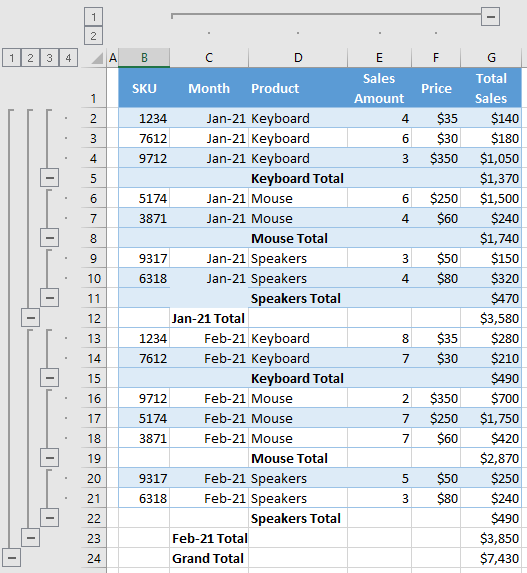
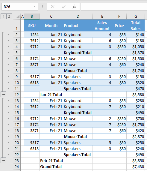
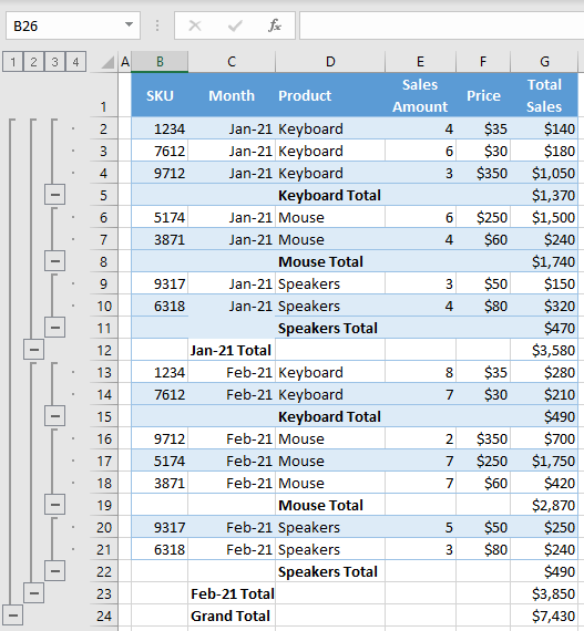
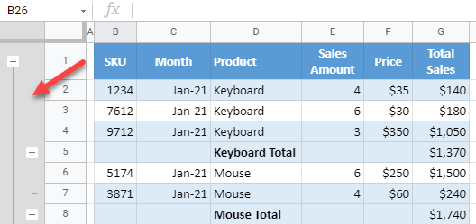
In the following example, we have total sales per month by product. Therefore, data are sorted by month and product and we have subtotals for each month, as we want to group data by month.

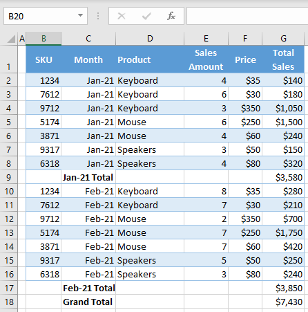
To group data for Jan-21 and Feb-21:

1. (1) Select data in the column that we want to group. In our case that is Jan-21, so we’ll select C2:C8. Then, in the Ribbon, (2) go to the Data tab, and in the Outline section, (3) click on the Group icon. (Note that you could also use a keyboard shortcut instead: ALT + SHIFT + right arrow).

3. In the new window, leave Rows selected since we want to group rows and click OK.

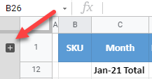
As a result, we get the outline bar on the left side with Jan-21 grouped.

4. If we want to collapse this group of data, we just need to click on the minus sign in the outline bar.

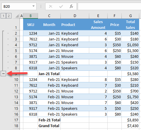
As shown in the picture below, all rows with Jan-21 in Column C are collapsed now and only the subtotal for this period remains visible.

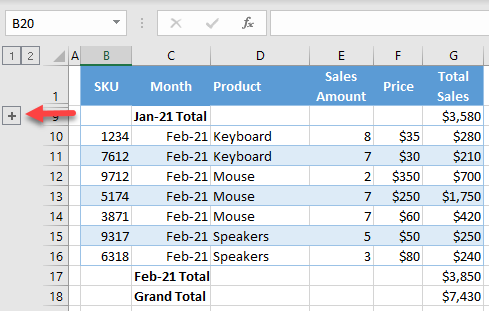
5. As in Step 4, we can expand the group (displaying rows) again, by clicking the plus sign. Following the exact same steps, we can also group data for Feb-21.

Group and Ungroup Multiple Levels of Data

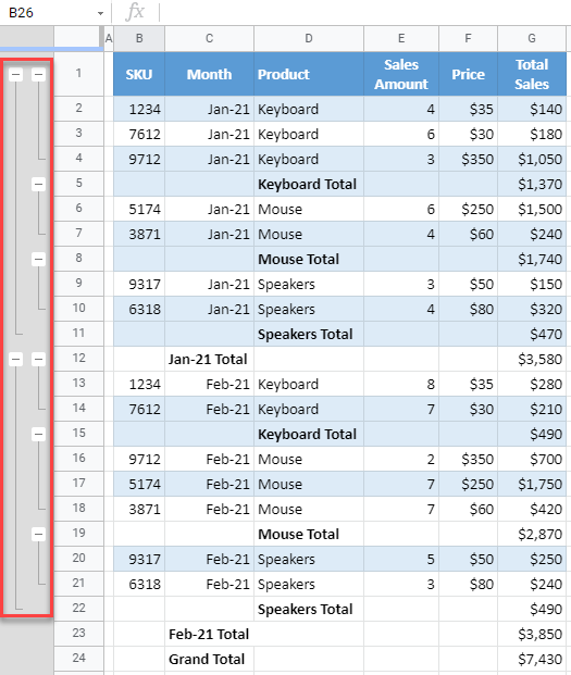
Say we want to add another level of data grouping: Product. First, add a subtotal for all products.

Currently, we have two groups for Month level and subtotals for months and products. Now, we want to add groups for products. We can do this in the exact same way as we did for months. In this case, we’ll add six groups of data, selecting – separately – Keyboard (D2:D4), Mouse (D6:D7), etc. As a result, our data and outline bars look like the picture below.

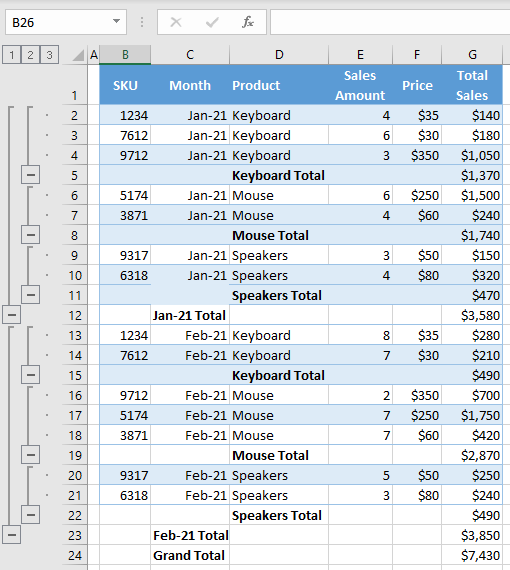
We now have two outline bars and the second one represents groups of products. Therefore, we can collapse all product groups, and have data organized in a way that displays only subtotals per month per product.

Group and Ungroup Rows Using Auto Outline

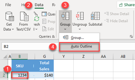
Instead of creating groups manually, we can also let Excel auto outline our data. This means that, if we have well-structured data, Excel will recognize groups and group data automatically.

To let Excel outline the data automatically, (1) click anywhere in the data, then in the Ribbon, (2) go to the Data tab, click on the arrow below the Group icon, and (3) choose Auto Outline.

We get almost the same outline bars as in the manual example because Excel can recognize data groups. The only difference is that the Auto Outline option creates one group more for Grand Total, which can collapse all the data except the Total.

To remove outline bars created by Auto Outline, (1) click anywhere in the data then in the Ribbon, (2) go to the Data tab, click on the arrow below the Ungroup icon, and choose (3) Clear Outline.

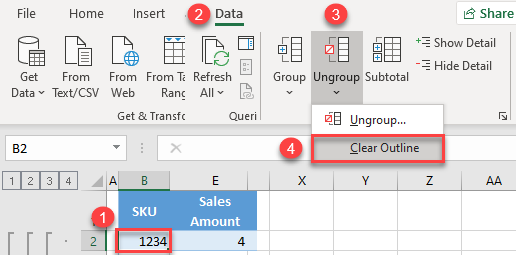
This will remove all outline bars and ungroup all data.

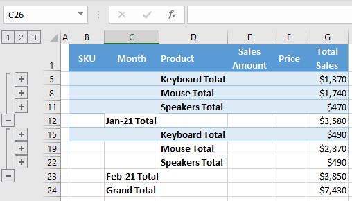
Expand and Collapse Entire Outline

Say we want to collapse the entire outline (for example, Month). In the outline bar, at the top, click on the outline bar number we want to collapse (in our case, outline level 2).

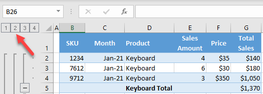
As a result, all rows with Jan-21 and Feb-21 are collapsed and only the totals are displayed.

If we want to expand the entire outline again, (1) click on Grand Total, then in the Ribbon, (2) go to the Data tab, and in the Outline section, (3) click on Show Detail.

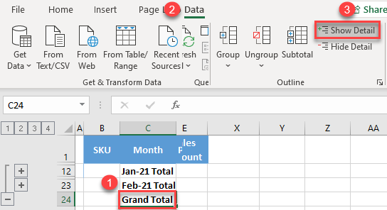
Now all data is visible again, and the Month outline is expanded.

Group and Ungroup Columns Manually

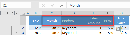
Similarly, we can also group columns in Excel. Say we want to display only SKU and the corresponding Total Sales.

1. Select all column headings that we want to group (in our case C1:F1).

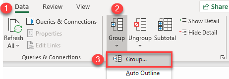
2. In the Ribbon, go to the Data tab, and in the Outline section, choose Group (or use the keyboard shortcut ALT + SHIFT + right arrow).

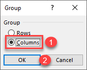
2. In the pop-up screen, (1) select Columns and (2) click OK.

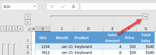
As a result, we will get a new outline bar, but this time for the columns.

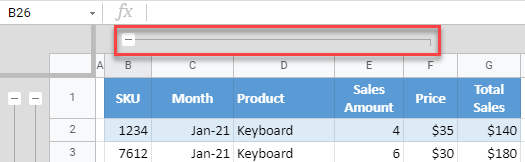
3. To collapse the group of columns, click on the minus sign at the end of the outline bar.

As a result, Columns C:F are collapsed.

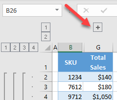
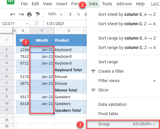
Group and Ungroup Rows in Google Sheets

In Google Sheets, we can only group rows manually, so let’s use the same example and see how to group data into the same categories. To group by month:

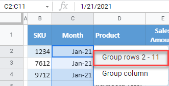
1. (1) Select all rows with Jan-21, then in the menu, (2) go to Data, and click on (3) Group.

2. In the new window beside the selection, click on Group rows 2 – 11.

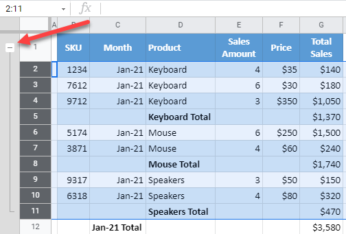
Jan-21 (Rows 2–11) are now grouped, and we can see the outline bar on the left side. The difference compared to Excel, is that the minus/plus sign for collapse/expand is a the top of each group.

3. To collapse Jan-21, click the minus sign at the top of the outline bar for months.

Now, data for the month are collapsed, and we can see only the Jan-21 Total row.

4. We now get the plus sign, so we can expand the group again.

5. Following these steps, we can also group Feb-21 and create a new outline for the Product data level. When we’re done, the data and outline bars should look like this:

Ungrouping data in Google Sheets works just like grouping.

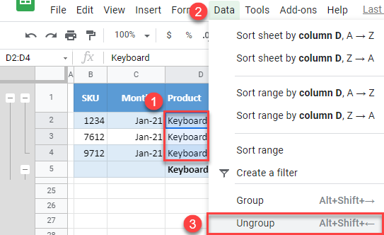
1. (1) Select the data we want to ungroup (Keyboard in Jan-21– cells D2:D4), then in the menu, (2) go to Data, and (3) click on Ungroup.

2. In the new window beside the selection, click on Ungroup rows 2 – 4.

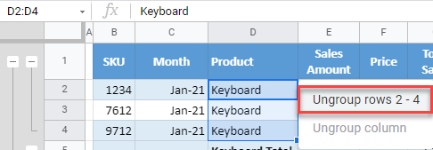
Those three rows are now ungrouped and removed from the outline bar.

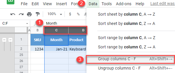
Group and Ungroup Columns in Google Sheets

Grouping columns can be done in a similar way to grouping rows.

Select Columns C:F, then in the menu, go to Data, and click on Group columns C – F.

Now, we get the outline bar for column grouping.

To ungroup columns, select Columns C:F, go to Data, and click on Ungroup columns C – F.

Источник

Grouping Rows in Excel

In Excel, organizing the large data by combining the subcategory data is called “grouping of rows.” When the number of items in line is not important, we can choose group rows that are not important but only see the subtotal of those rows. On the other hand, when the data rows are huge, scrolling down and reading the report may lead to a wrong understanding, so the grouping of rows helps us hide the unwanted numbers of rows.

The number of rows is also lengthy when the worksheet contains detailed information or data. However, report readers of the data do not want to see long rows. Instead, they want to see a clear view, but at the same time, if they require any other detailed information, they need just a button to expand or collapse them as needed.

This article will show you how to group rows in Excel with expand/collapse to maximize the report viewing technique.

Grouping Rows in Excel
- How to Group Rows in Excel with Expand/Collapse?
  - Group by Using Shortcut Key
  - Example #1 – Using Auto Outline
  - Example #2 – Using Subtotals
- Things to Remember here
- Recommended Articles

How to Group Rows in Excel with Expand/Collapse?

You can download this Group Rows Excel Template here – Group Rows Excel Template

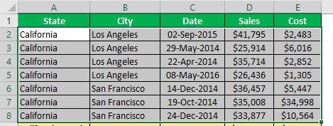
For example, look at the below data.

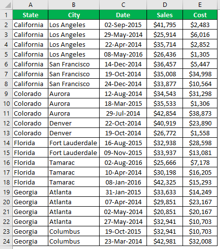
We have city and state-related sales and cost data in the table above. Still, when we look at the first two rows of the data, we have “California” state and the city is “Los Angeles,” but sales happened on different dates. Hence, as a report reader, everyone prefers to read the state-wise sales and city-wise sales in a single column, so we can create a single line summary view by grouping the rows.

Follow the below steps to group rows in excel.

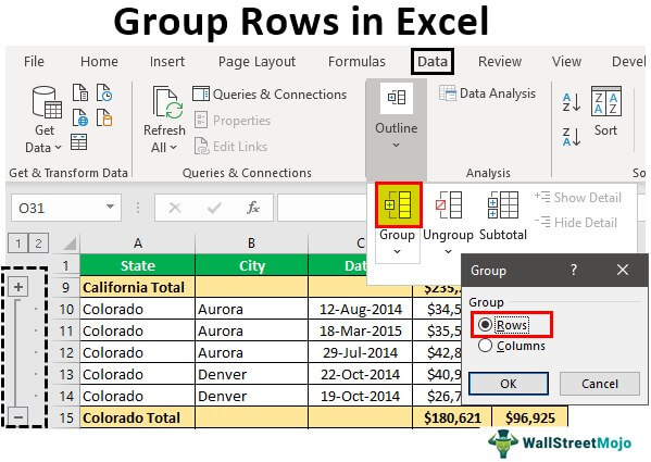
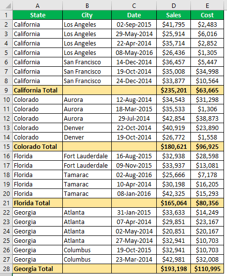
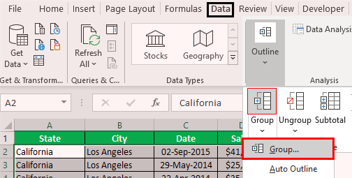
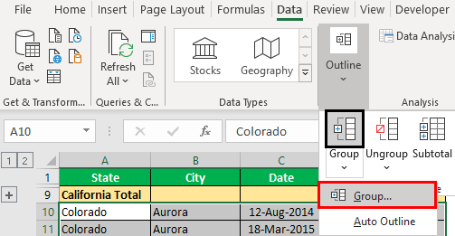
First, we must create a subtotal like the one below.
We must select the first state rows (California state), excluding subtotals.
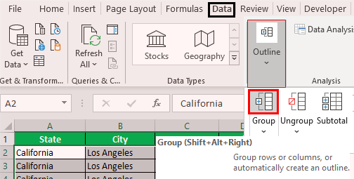
Then, go to the Data tab and choose the “Group” option.
Click on the drop-down list in excel of “Group” and choose “Group” again.
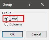
Now, it may ask whether to group rows or columns. Since we are grouping Rows, we must choose Rows and click on OK.
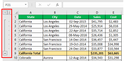
The moment we click on OK, we can see a joint line on the left-hand side.
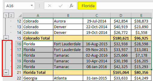
Then, we must click on the minus icon and see the magic.

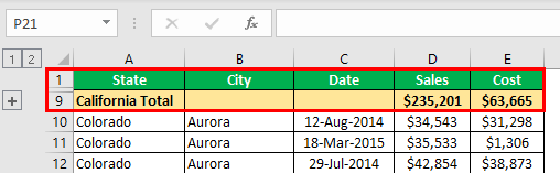
Now, we can see the total summary for the city California. Again, if we want to see a detailed overview of the city, we can click on the plus icon to expand the view.
Now again, select the city Colorado and click on the Group option.
As a result, it will group for the Colorado state.

Group by Using Shortcut Key

With a simple shortcut in excelAn Excel shortcut is a technique of performing a manual task in a quicker way.read more, we can easily group selected rows or columns. The shortcut key to group the data is “SHIFT + ALT + Right Arrow key.”

First, we must select the rows that need to be grouped.

To group these rows, we must press the shortcut key “SHIFT + ALT + Right Arrow key.“

In the above, we have seen how to group the data and row with expanding and collapse options using the “PLUS” and “MINUS” icons.

The only problem with the above method is that we need to do this for each state individually, so this takes a lot of time when there are many states. So, what would be your reaction if we say you can group with just one click?

Amazing. Using the “Auto Outline,” we can automatically group the data.

Example #1 – Using Auto Outline

First we need to create subtotal rows.

Now, we must place a cursor inside the data range. Under the “Group” drop-down, we can see one more option other than “Group,” which is “Auto Outline.”

The moment we click on this “Auto Outline” option, it will group all the rows above the subtotal row.

How cool is this??? Very cool, isn’t it??

Example #2 – Using Subtotals

If grouping the rows for the individual city is the one problem, then even before grouping rows, there is another problem: adding subtotal rows.

When there are hundreds of states, it is a tough task to create a subtotal row for each state separately, so we can use the “Subtotal” option to create a subtotal for the selected column quickly.

For example, we had the data like the below before creating the subtotal.

Under the “Data” tab, we have an option called “Subtotal” right next to the “Group” option.

Click on this option by selecting any of the cells of the data range. It will show the below option first up.

First, select the column that needs a subtotal. In this example, we need subtotal for “State,” so choose the same from the drop-down list of “At each change in.”

Next, we need to select the function type since we add all the values to choose “Sum” function in excel.

Now, select the columns that need to be summed. We need the summary of the “Sales“and “Cost” columns, so choose the same. Click on “OK.”

We will have subtotal rows shortly.

Did you notice one special thing from the above image???

It has automatically grouped rows for us!!!!

Things to Remember here

The shortcut key for grouping rows is the “Shift + ALT + Right Arrow” key.
We should sort subtotal that needs data.
The “Auto Outline” option can group all the rows above the subtotal row.

Развернуть / свернуть строки или столбцы в Excel и Google Таблицах

В этой статье вы узнаете, как разворачивать и сворачивать строки или столбцы, группируя их в Excel и Google Таблицах.

Excel позволяет нам группировать и разгруппировать данные, что позволяет нам разворачивать или сворачивать строки и столбцы, чтобы лучше организовать наши электронные таблицы. Это возможно группировка данных вручную или используя Авто контур вариант.

Группировка и разгруппировка строк вручную

Если мы хотим группировать строки в Excel нам необходимо организовать данные таким образом, чтобы они были совместимы с функцией группировки в Excel. Это означает, что нам нужно несколько уровней информации отсортированы правильно а также промежуточные итоги для каждого уровня информации, которую мы хотим сгруппировать. Кроме того, в данных не должно быть пустых строк или пробелов.

В следующем примере у нас есть общий объем продаж за месяц по продуктам. Таким образом, данные сортируются по месяцам и продуктам, и у нас есть промежуточные итоги за каждый месяц, так как мы хотим группировать данные по месяцам.

Сгруппировать данные для Янв-21 а также 21 февраля:

1. (1) Выберите данные в столбце, который мы хотим сгруппировать. В нашем случае это Янв-21, поэтому мы выберем C2: C8. Затем в Лента, (2) перейти к Данные вкладка и в Контур раздел, (3) нажмите на Группа значок. (Обратите внимание, что вместо этого вы также можете использовать сочетание клавиш: ALT + SHIFT + стрелка вправо).

3. В новом окне оставьте строки выбранными поскольку мы хотим сгруппировать строки и щелкнуть Ok.

В результате мы получаем полосу контура слева с Янв-21 сгруппированы.

4. Если мы хотим свернуть эту группу данных, нам просто нужно нажмите на знак минус в панели структуры.

Как показано на рисунке ниже, все строки с Янв-21 в столбце C теперь свернуты, и остается видимой только промежуточный итог за этот период.

5. Как и в шаге 4, мы можем расширить группу (отображение строк) снова, нажав на знак плюса. Следуя точно таким же шагам, мы также можем сгруппировать данные для 21 февраля.

Группировка и разгруппировка нескольких уровней данных

Допустим, мы хотим добавить еще один уровень группировки данных: Продукт. Сначала добавьте промежуточный итог для всех продуктов.

В настоящее время у нас есть две группы для Месяц уровень и промежуточные итоги по месяцам и продуктам. Теперь мы хотим добавить группы для продуктов. Мы можем делать это точно так же, как делали это месяцами. В этом случае мы добавим шесть групп данных, выбирая — отдельно — Клавиатура (D2: D4), Мышь (D6: D7) и т. Д. В результате наши данные и панели схемы выглядят так, как показано на рисунке ниже.

Теперь у нас есть две полосы структуры, а вторая представляет группы продуктов. Следовательно, мы можем свернуть все группы продуктов и организовать данные таким образом, чтобы отображались только промежуточные итоги за месяц для каждого продукта.

Группировка и разгруппировка строк с помощью автоматического контура

Вместо того, чтобы создавать группы вручную, мы также можем позволить Excel автоматический контур наши данные. Это означает, что, если у нас есть хорошо структурированные данные, Excel автоматически распознает группы и групповые данные.

Чтобы Excel автоматически выделял данные, (1) щелкните в любом месте данных, то в Лента, (2) перейти к Данные вкладку, нажмите на стрелка под значком группы, и (3) выбираем Авто контур.

Мы получаем почти те же полосы контура, что и в ручном примере, потому что Excel может распознавать группы данных. Единственное отличие состоит в том, что опция Auto Outline создает еще одну группу для общего итога, которая может свернуть все данные, кроме итога.

К удалить полосы контура создано Auto Outline, (1) щелкните в любом месте данных затем в Лента, (2) перейти к Данные вкладку, нажмите на стрелка под значком Разгруппировать, и выберите (3) Четкий контур.

Это удалит все контурные полосы и разгруппирует все данные.

Развернуть и свернуть всю схему

Скажем, мы хотим свернуть всю схему (Например, Месяц). На панели структуры вверху нажмите на номер панели контура мы хотим свернуть (в нашем случае уровень 2).

В результате все строки с Янв-21 а также 21 февраля свернуты, и отображаются только итоги.

Если мы хотим снова развернуть весь контур, (1) нажмите Общая сумма, то в Лента, (2) перейти к Данные вкладка и в Контур раздел, (3) нажмите Показать детали.

Теперь все данные снова видны, а значок Месяц контур расширен.

Сгруппировать и разгруппировать столбцы вручную

Точно так же мы можем также группировать столбцы в Excel. Скажем, мы хотим отображать только SKU и соответствующие Тотальная распродажа.

1. Выделите все заголовки столбцов, которые мы хотим сгруппировать (в нашем случае C1: F1).

2. В Лента, перейдите в Данные вкладка и в Контур раздел, выберите Группа (или воспользуйтесь сочетанием клавиш ALT + SHIFT + стрелка вправо).

2. Во всплывающем экране (1) выберите столбцы и (2) нажмите ОК.

В результате мы получим новую полосу контура, но на этот раз для столбцов.

3. Чтобы свернуть группу столбцов, нажмите на знак минус в конце панели контура.

В результате столбцы C: F свернуты.

В Google Таблицах мы можем группировать строки только вручную, поэтому давайте воспользуемся тем же примером и посмотрим, как сгруппировать данные по одним и тем же категориям. Чтобы сгруппировать по месяцам:

1. (1) Sвыбрать все строки с Янв-21, затем в меню (2) перейдите к Данныеи нажмите (3) Группа.

2. В новом окне рядом с выбором нажмите Сгруппируйте ряды 2-11.

Янв-21 (Строки 2-11) теперь сгруппированы, и мы можем видеть полосу контура с левой стороны. Разница по сравнению с Excel заключается в том, что знак минус / плюс для свертывания / развертывания находится вверху каждой группы.

3. Свернуть Янв-21, щелкните знак минус вверху панели структуры в течение месяцев.

Теперь данные за месяц свернуты, и мы можем видеть только Янв-21 Итого ряд.

4. Теперь у нас есть знак плюса, так что мы можем снова расширить группу.

5. Следуя этим шагам, мы также можем сгруппировать 21 февраля и создайте новый контур для Продукт уровень данных. Когда мы закончим, панели данных и структуры должны выглядеть следующим образом:

Разгруппировка данных в Google Таблицах работает так же, как группировка.

1. (1) Sвыберите данные, которые мы хотим разгруппировать (Клавиатура в Янв-21— ячейки D2: D4), затем в меню (2) перейдите в Данные, и (3) нажмите на Разгруппировать.

2. В новом окне рядом с выбором нажмите Разгруппируйте строки 2–4.

Эти три строки теперь разгруппированы и удалены с панели структуры.

Сгруппировать и разгруппировать столбцы в Google Таблицах

Группировка столбцов можно сделать аналогично группировке строк.

Выберите столбцы C: F, затем в меню перейдите к Данныеи нажмите Сгруппировать столбцы C — F.

Теперь у нас есть панель контура для группировки столбцов.

Чтобы разгруппировать столбцы, выберите столбцы C: F, перейти к Данныеи нажмите Разгруппировать столбцы C — F.

Источник

Need more help?

See Also

Need more help?

How do you expand and collapse multiple columns in Excel?

What is the shortcut to expand all collapsed rows in Excel?

How do you make Excel cells expand to fit text automatically?

How do you expand columns in Excel?

How does a Vlookup work?

Can you do a sum of highlighted cells in Excel?

How do I widen all rows in Excel?

How do I expand rows in Excel spreadsheet?

Where is the expand button in Excel?

How do you flash fill in Excel?

What is the shortcut to expand all columns in Excel?

How do you expand a table in Excel?

How do you do a VLOOKUP for beginners?

Is VLOOKUP hard to learn?

How do I sum colored cells in Excel without VBA?

Can you create a formula in Excel based on color?

How do I sum colored cells in Excel using Countif?

How do I make my Excel spreadsheet fit on one page?

How do I find collapse rows in Excel?

How do you show collapsed rows in Excel?

Group and Ungroup Rows Manually

Group and Ungroup Multiple Levels of Data

Group and Ungroup Rows Using Auto Outline

Expand and Collapse Entire Outline

Group and Ungroup Columns Manually

Group and Ungroup Rows in Google Sheets

Group and Ungroup Columns in Google Sheets

Grouping Rows in Excel

Table of contents

How to Group Rows in Excel with Expand/Collapse?

Group by Using Shortcut Key

Example #1 – Using Auto Outline

Example #2 – Using Subtotals

Things to Remember here

Recommended Articles

Развернуть / свернуть строки или столбцы в Excel и Google Таблицах

Группировка и разгруппировка строк вручную

Группировка и разгруппировка нескольких уровней данных

Группировка и разгруппировка строк с помощью автоматического контура

Развернуть и свернуть всю схему

Сгруппировать и разгруппировать столбцы вручную

Сгруппировать и разгруппировать столбцы в Google Таблицах