Exclusive or in excel

The Excel XOR function returns a logical “exclusive OR” of all arguments and provides TRUE or FALSE output.

If you use two logical tests, XOR will return TRUE if either logical test evaluates to TRUE and return FALSE if both logical values are TRUE.

XOR returns FALSE if neither logical is TRUE.

Syntax, Arguments, and return value

The function uses the following syntax:

=XOR(logical1, logical2,…..)

XOR uses one required and up to a maximum of 254 optional arguments.

• logical1: Expression or constant that returns TRUE or FALSE.
• logical2 [optional]: Expression or constant that returns TRUE or FALSE.

All arguments will evaluate to logical values such as TRUE or FALSE, or in arrays or references that contain logical values.

Return value: We use the XOR function to perform exclusive OR, where the return value is TRUE or FALSE.

Look at the differences between XOR and the OR function. XOR function provides exclusive OR, OR function provides inclusive OR. If you add two logical values as XOR function arguments, the function returns TRUE only if one of the logical is TRUE. If both logical is TRUE, the result is FALSE.

At first, the definition seems complicated, so here is a real-life example. For the sake of simplicity, we have two logicals:

• logical1: the output of “I’ll be at my office until 8 pm.“
• logical2: the output of “I’ll be at the cinema until 8 pm.”

=XOR("I'll be at my office until 8 pm", "I'll be at the cinema until 8 pm")

Based on the XOR function definition: You can’t watch your favorite movie at the cinema and simultaneously work on your project at the office. (If you have superhero skills, you can do that, but set this case aside)

If you are at the office until 8 pm OR at the cinema until 8 pm, the expression is TRUE. In any other cases, the XOR function returns FALSE.

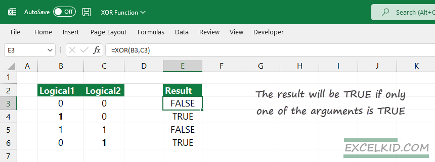
Exclusive OR function with two logical values

If you are working with two arguments, the formula is the following:

=XOR(A1, B1)

In this case, the result will be TRUE if only one of the arguments is TRUE. In all other cases, the result is FALSE.

Working with multiple logical values

Let us see what will happen if you use the XOR function with more than two arguments (logical values).

If you want to simplify the rule, keep in mind: The XOR function returns TRUE when the number of TRUE arguments is odd and FALSE when the number of TRUE arguments is even.

In the example, enter the following formula in G3:

=XOR(B3,C3,D3,E3)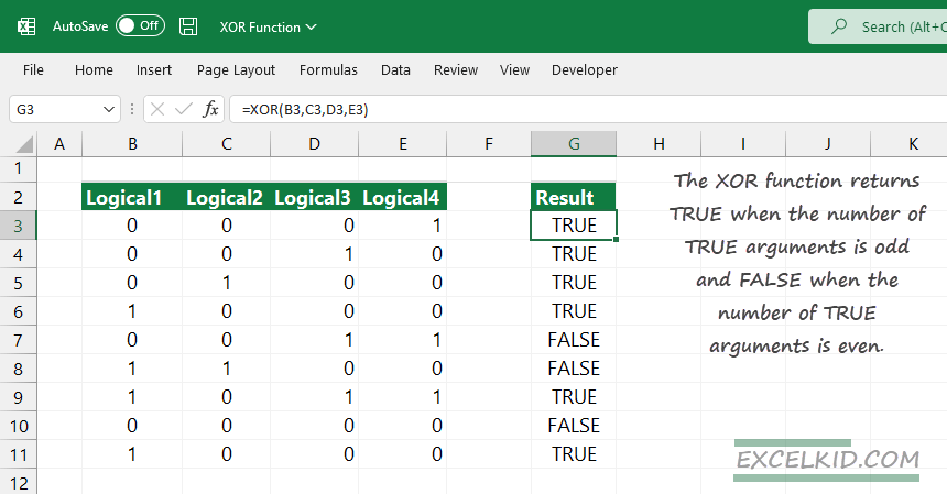

XOR will aggregate the logical test results in each row and return TRUE or FALSE. In G3, the result is TRUE because the number of TRUE arguments is odd (1). Following this logic, in cell G9, the result is TRUE since the number of TRUE values is an odd number (3). This method works based on the algorithm mentioned above in the case of 10+ logical values.

Summary

• Excel will evaluate the XOR function arguments to TRUE/FALSE or 1/0.
• XOR returns TRUE when the number of TRUE arguments is odd, else gets FALSE.
• The function returns a #VALUE error if the result does not contain logical values.

The XOR function performs what is called «exclusive OR», in contrast to the «inclusive OR» performed by the OR function. Whereas the OR function returns true if any input is TRUE, XOR only returns TRUE in specific cases. In the simplest case, with just two logical statements, XOR returns TRUE only if one of the logicals is TRUE. If both values are TRUE, XOR returns FALSE.

The concept of exclusive OR is more common in the world of programming. In plain English, you can think of a sentence like this: «I’m either going to visit New York or San Francisco this summer». Nothing prevents the speaker from visiting both, but the meaning is clearly that they plan to visit only one or the other. If they visit one or the other, the original statement is TRUE. If they visit neither or both, the original statement is FALSE.

Example #1 — two values

In the example shown, the formula in D5, copied down, is:

=XOR(B5,C5)

At each row, XOR only returns TRUE when B5 and C5 contain a single TRUE or equivalent value.

Example #2 — more than two values

With more than 2 values, the behavior of XOR is a bit different. With three or more logicals, XOR only returns TRUE when the number of TRUE values is odd, as shown in the following example:

In this example, XOR is given a range with five values in a single argument instead of five separate arguments. The formula in G6 copied down is:

=XOR(B6:F6)

The result is TRUE only when the number of TRUE values columns B through F is an odd number.

Notes

• Logical arguments must evaluate to TRUE or FALSE, 1 or 0, or be references that contain logical values.
• XOR returns #VALUE! if no logical values are found.
• With more than two logicals, XOR returns TRUE when the number of TRUE logicals is odd, and FALSE if not.
• XOR was introduced in Excel 2013.

Функция OR (ИЛИ) в Excel используется для сравнения двух условий.

Что возвращает функция

Возвращает логическое значение TRUE (Истина), при выполнении условий сравнения в функции и отображает FALSE (Ложь), если условия функции не совпадают.

Синтаксис

=OR(logical1, [logical2],…) — английская версия

=ИЛИ(логическое_значение1;[логическое значение2];…) — русская версия

Аргументы функции

• logical1 (логическое_значение1) — первое условие которое оценивает функция по логике TRUE или FALSE;
• [logical2] ([логическое значение2]) — (не обязательно) это второе условие которое вы можете оценить с помощью функции по логике TRUE или FALSE.

Дополнительная информация

• Функция OR (ИЛИ) может использоваться с другими формулами.

Например, в функции IF (ЕСЛИ) вы можете оценить условие и затем присвоить значение, когда данные отвечают условиям логики TRUE или FALSE. Используя функцию вместе с IF (ЕСЛИ), вы можете тестировать несколько условий оценки значений за раз.

Например, если вы хотите проверить значение в ячейке А1 по условию: “Если значение больше “0” или меньше “100” то… “ — вы можете использовать следующую формулу:

=IF(OR(A1>100,A1<0),”Верно”,”Неверно”) — английская версия

=ЕСЛИ(ИЛИ(A1>100;A1<0);»Верно»;»Неверно») — русская версия

• Аргументы функции должны быть логически вычислимы по принципу TRUE или FALSE;
• Текст и пустые ячейки игнорируются функцией;
• Если вы используете функцию с не логически вычисляемыми значениями — она выдаст ошибку;
• Вы можете тестировать максимум 255 условий в одной формуле.

Примеры использования функции OR (ИЛИ) в Excel

Пример 1. Используем аргументы TRUE и FALSE в функции OR (ИЛИ)

Вы можете использовать TRUE/FALSE в качестве аргументов. Если любой из них соответствует условию TRUE, функция выдаст результат TRUE. Если оба аргумента функции соответствуют условию FALSE, функция выдаст результат FALSE.

Она может использовать аргументы TRUE и FALSE в кавычках.

Пример 2. Используем ссылки на ячейки, содержащих TRUE/FALSE

Вы можете использовать ссылки на ячейки со значениями TRUE или FALSE. Если любое значение из ссылок соответствует условиям TRUE, функция выдаст TRUE.

Пример 3. Используем условия с функцией OR (ИЛИ)

Вы можете проверять условия с помощью функции OR (ИЛИ). Если любое из условий соответствует TRUE, функция выдаст результат TRUE.

Пример 4. Используем числовые значения с функцией OR (ИЛИ)

Число “0” считается FALSE в Excel по умолчанию. Любое число, выше “0”, считается TRUE (оно может быть положительным, отрицательным или десятичным числом).

Пример 5. Используем функцию OR (ИЛИ) с другими функциями

Вы можете использовать функцию OR (ИЛИ) с другими функциями для того, чтобы оценить несколько условий.

На примере ниже показано, как использовать функцию вместе с IF (ЕСЛИ):

На примере выше, мы дополнительно используем функцию IF (ЕСЛИ) для того, чтобы проверить несколько условий. Формула проверяет значение ячеек А2 и A3. Если в одной из них значение более чем “70”, то формула выдаст “TRUE”.

There are many ways to add logical decision-making to your Excel spreadsheets. In addition to the standard logical operators in Excel (=, <, >, <>, <=, >=), Excel has compound logical functions which let you evaluate multiple conditions at once. The AND, OR, XOR, and NOT functions in Excel let you evaluate many logical conditions and simply return TRUE or FALSE depending on the function. Because they return TRUE or FALSE, these functions are commonly used with IF functions.

To get detailed information about a function, click its name in the first column.

Note: Version markers indicate the version of Excel a function was introduced. These functions aren’t available in earlier versions. For example, a version marker of 2013 indicates that this function is available in Excel 2013 and all later versions.

Function	Description
AND function	Returns TRUE if all of its arguments are TRUE
BYCOL function	Applies a LAMBDA to each column and returns an array of the results
BYROW function	Applies a LAMBDA to each row and returns an array of the results
FALSE function	Returns the logical value FALSE
IF function	Specifies a logical test to perform
IFERROR function	Returns a value you specify if a formula evaluates to an error; otherwise, returns the result of the formula
IFNA function	Returns the value you specify if the expression resolves to #N/A, otherwise returns the result of the expression
IFS function	Checks whether one or more conditions are met and returns a value that corresponds to the first TRUE condition.
LAMBDA function	Create custom, reusable functions and call them by a friendly name
LET function	Assigns names to calculation results
MAKEARRAY function	Returns a calculated array of a specified row and column size, by applying a LAMBDA
MAP function	Returns an array formed by mapping each value in the array(s) to a new value by applying a LAMBDA to create a new value
NOT function	Reverses the logic of its argument
OR function	Returns TRUE if any argument is TRUE
REDUCE function	Reduces an array to an accumulated value by applying a LAMBDA to each value and returning the total value in the accumulator
SCAN function	Scans an array by applying a LAMBDA to each value and returns an array that has each intermediate value
SWITCH function	Evaluates an expression against a list of values and returns the result corresponding to the first matching value. If there is no match, an optional default value may be returned.
TRUE function	Returns the logical value TRUE
XOR function	Returns a logical exclusive OR of all arguments

Important: The calculated results of formulas and some Excel worksheet functions may differ slightly between a Windows PC using x86 or x86-64 architecture and a Windows RT PC using ARM architecture. Learn more about the differences.

See Also

Excel functions (by category)

Excel functions (alphabetical)

Date yes Add (Subtract) Days to a Date Concatenate Dates Convert Date to Number Convert Date to Text Month Name to Number Create Date Range from Dates Day Number of Year Month Name from Date First Day of Month Add (Subtract) Weeks to a Date If Functions with Dates Max Date Number of Days Between Dates Number of Days in a Month Number of Weeks Between Dates Number of Years Between Dates Split Date & Time into Separate Cells Countdown Remaining Days Insert Dates Random Date Generator Using Dynamic Ranges — Year to Date Values Add (Subtract) Years to a Date Date Formula Examples Extract Day from Date Get Day Name from Date Count Days Left in Month / Year Count Workdays Left in Month / Year Get Last Day of Month Last Business Day of Month / Year Number of Work / Business Days in Month Weekday Abbreviations Auto Populate Dates Number of Months Between Dates Quarter from a Date Years of Service Change Date Format Compare Dates Time yes Add (Subtract) Hours to Time Add (Subtract) Minutes to Time Add (Subtract) Seconds to Time Add Up time (Total Time) Time Differences Change Time Format Convert Minutes to Hours Convert Time to Decimal Convert Time to Hours Convert Time to Minutes Convert Time to Seconds Military Time Round Time to Nearest 15 Minutes Overtime Calculator Number of Hours Between Times Convert Seconds to Minutes, Hours, or Time Count Hours Worked Time Differences Time Format — Show Minutes Seconds Text yes Add Commas to Cells Get First Word from Text Capitalize First Letter Clean & Format Phone #s Remove Extra Trailing / Leading Spaces Add Spaces to Cell Assign Number Value to Text Combine Cells with Comma Combine First and Last Names Convert Text String to Date Convert Text to Number Extract Text From Cell Get Last Word Remove Unwated Characters Extract Text Before or After Character How to Split Text String by Space, Comma, & More Remove Special Characters Remove First Characters from Left Substitute Multiple Values Switch First & Last Names w/ Commas Remove Specific Text from a Cell Extract Text Between Characters (Ex. Parenthesis) Add Leading Zeros to a Number Remove Line Breaks from Text Remove all Numbers from Text Reverse Text Remove Non-Numeric Characters Remove Last Character(s) From Right Separate First and Last Names Separate Text & Numbers Round yes Round Formulas Round Price to Nearest Dollar or Cent Round to Nearest 10, 100, or 1000 Round to Nearest 5 or .5 Round Percentages Round to Significant Figures Count yes Count Blank and Non-blank Cells Count Cells Between Two Numbers Count Cells not Equal to Count if Cells are in Range Count Times Word Appears in Cell Count Words in Cell Count Specific Characters in Column Count Total Number of Characters in Column Count Cells that Equal one of two Results Count Cells that do not Contain Count Cells that Contain Specific Text Count Unique Values in Range Countif — Multiple Criteria Count Total Number of Cells in Range Count Cells with Any Text Count Total Cells in a Table Lookup yes Two Dimensional VLOOKUP VLOOKUP Simple Example Vlookup — Multiple Matches Case Sensitive Lookup Case Sensitive VLOOKUP Sum if — VLOOKUP Case Sensitive Lookup Case Sensitive VLOOKUP Find Duplicates w/ VLOOKUP or MATCH INDEX MATCH MATCH Lookup — Return Cell Address (Not Value) Lookup Last Value in Column or Row Reverse VLOOKUP (Right to Left) Risk Score Bucket with VLOOKUP Sum with a VLOOKUP Function VLOOKUP & INDIRECT VLOOKUP Concatenate VLOOKUP Contains (Partial Match) 17 Reasons Why Your XLOOKUP is Not Working Double (Nested) XLOOKUP — Dynamic Columns IFERROR (& IFNA) XLOOKUP Lookup Min / Max Value Nested VLOOKUP Top 11 Alternatives to VLOOKUP (Updated 2022!) VLOOKUP – Dynamic Column Reference VLOOKUP – Fix #N/A Error VLOOKUP – Multiple Sheets at Once VLOOKUP & HLOOKUP Combined VLOOKUP & MATCH Combined VLOOKUP Between Worksheets or Spreadsheets VLOOKUP Duplicate Values VLOOKUP Letter Grades VLOOKUP Return Multiple Columns VLOOKUP Returns 0? Return Blank Instead VLOOKUP w/o #N/A Error XLOOKUP Multiple Sheets at Once XLOOKUP Between Worksheets or Spreadsheets XLOOKUP by Date XLOOKUP Duplicate Values XLOOKUP Multiple Criteria XLOOKUP Return Multiple Columns XLOOKUP Returns 0? Return Blank Instead XLOOKUP Text XLOOKUP with IF XLOOKUP With If Statement Misc. yes Sort Multiple Columns Use Cell Value in Formula Percentage Change Between Numbers Percentage Breakdown Rank Values Add Spaces to Cell CAGR Formula Average Time Decimal Part of Number Integer Part of a Number Compare Items in a List Dealing with NA() Errors Get Worksheet Name Wildcard Characters Hyperlink to Current Folder Compound Interest Formula Percentage Increase Create Random Groups Sort with the Small and Large Functions Non-volatile Function Alternatives Decrease a Number by a Percentage Calculate Percent Variance Profit Margin Calculator Convert Column Number to Letter Get Full Address of Named Range Insert File Name Insert Path Latitute / Longitude Functions Replace Negative Values Reverse List Range Convert State Name to Abbreviation Create Dynamic Hyperlinks Custom Sort List with Formula Data Validation — Custom Formulas Dynamic Sheet Reference (INDIRECT) Reference Cell in Another Sheet or Workbook Get Cell Value by Address Get Worksheet Name Increment Cell Reference List Sheet Names List Skipped Numbers in Sequence Return Address of Max Value in Range Search by Keywords Select Every Other (or Every nth) Row Basics yes Cell Reference Basics — A1, R1C1, 3d, etc. Add Up (Sum) Entire Column or Row Into to Dynamic Array Formulas Conversions yes Convert Time Zones Convert Celsius to Fahrenheit Convert Pounds to Kilograms Convert Time to Unix Time Convert Feet to Meters Convert Centimeters to Inches Convert Kilometers to Miles Convert Inches to Feet Convert Date to Julian Format Convert Column Letter to Number Tests yes Test if a Range Contains any Text Test if any Cell in Range is Number Test if a Cell Contains a Specific Value Test if Cell Contains Any Number Test if Cell Contains Specific Number Test if Cell is Number or Text If yes Percentile If Subtotal If Sumproduct If Large If and Small If Median If Concatentate If Max If Rank If TEXTJOIN If Sum yes Sum if — Begins With / Ends With Sum if — Month or Year to Date Sum if — By Year Sum if — Blank / Non-Blank Sum if — Horizontal Sum Count / Sum If — Cell Color INDIRECT Sum Sum If — Across Multiple Sheets Sum If — By Month Sum If — Cells Not Equal To Sum If — Not Blank Sum if — Between Values Sum If — Week Number Sum Text Sum if — By Category or Group Sum if — Cell Contains Specific Text (Wildcards) Sum if — Date Rnage Sum if — Dates Equal Sum if — Day of Week Sum if — Greater Than Sum if — Less Than Average yes Average Non-Zero Values Average If — Not Blank Average — Ignore 0 Average — Ignore Errors Math yes Multiplication Table Cube Roots nth Roots Square Numbers Square Roots Calculations yes Calculate a Ratio Calculate Age KILLLLLLL Calculate Loan Payments GPA Formula Calculate VAT Tax How to Grade Formulas Find yes Find a Number in a Column / Workbook Find Most Frequent Numbers Find Smallest n Values Find nth Occurance of Character in Text Find and Extract Number from String Find Earliest or Latest Date Based on Criteria Find First Cell with Any Value Find Last Row Find Last Row with Data Find Missing Values Find Largest n Values Most Frequent Number Conditional Formatting yes Conditional Format — Dates & Times Conditional Format — Highlight Blank Cells New Functions XLOOKUP Replaces VLOOKUP, HLOOKUP, and INDEX / MATCH Logical yes AND Checks whether all conditions are met. TRUE/FALSE IF If condition is met, do something, if not, do something else. IFERROR If result is an error then do something else. NOT Changes TRUE to FALSE and FALSE to TRUE. OR Checks whether any conditions are met. TRUE/FALSE XOR Checks whether one and only one condition is met. TRUE/FALSE Lookup & Reference yes FALSE The logical value: FALSE. TRUE The logical value: TRUE. ADDRESS Returns a cell address as text. AREAS Returns the number of areas in a reference. CHOOSE Chooses a value from a list based on it’s position number. COLUMN Returns the column number of a cell reference. COLUMNS Returns the number of columns in an array. HLOOKUP Lookup a value in the first row and return a value. HYPERLINK Creates a clickable link. INDEX Returns a value based on it’s column and row numbers. INDIRECT Creates a cell reference from text. LOOKUP Looks up values either horizontally or vertically. MATCH Searches for a value in a list and returns its position. OFFSET Creates a reference offset from a starting point. ROW Returns the row number of a cell reference. ROWS Returns the number of rows in an array. TRANSPOSE Flips the oriention of a range of cells. VLOOKUP Lookup a value in the first column and return a value. Date & Time yes DATE Returns a date from year, month, and day. DATEDIF Number of days, months or years between two dates. DATEVALUE Converts a date stored as text into a valid date DAY Returns the day as a number (1-31). DAYS Returns the number of days between two dates. DAYS360 Returns days between 2 dates in a 360 day year. EDATE Returns a date, n months away from a start date. EOMONTH Returns the last day of the month, n months away date. HOUR Returns the hour as a number (0-23). MINUTE Returns the minute as a number (0-59). MONTH Returns the month as a number (1-12). NETWORKDAYS Number of working days between 2 dates. NETWORKDAYS.INTL Working days between 2 dates, custom weekends. NOW Returns the current date and time. SECOND Returns the second as a number (0-59) TIME Returns the time from a hour, minute, and second. TIMEVALUE Converts a time stored as text into a valid time. TODAY Returns the current date. WEEKDAY Returns the day of the week as a number (1-7). WEEKNUM Returns the week number in a year (1-52). WORKDAY The date n working days from a date. WORKDAY.INTL The date n working days from a date, custom weekends. YEAR Returns the year. YEARFRAC Returns the fraction of a year between 2 dates. Engineering yes CONVERT Convert number from one unit to another. Financial yes FV Calculates the future value. PV Calculates the present value. NPER Calculates the total number of payment periods. PMT Calculates the payment amount. RATE Calculates the interest Rate. NPV Calculates the net present value. IRR The internal rate of return for a set of periodic CFs. XIRR The internal rate of return for a set of non-periodic CFs. PRICE Calculates the price of a bond. YIELD Calculates the bond yield. INTRATE The interest rate of a fully invested security. Information yes CELL Returns information about a cell. ERROR.TYPE Returns a value representing the cell error. ISBLANK Test if cell is blank. TRUE/FALSE ISERR Test if cell value is an error, ignores #N/A. TRUE/FALSE ISERROR Test if cell value is an error. TRUE/FALSE ISEVEN Test if cell value is even. TRUE/FALSE ISFORMULA Test if cell is a formula. TRUE/FALSE ISLOGICAL Test if cell is logical (TRUE or FALSE). TRUE/FALSE ISNA Test if cell value is #N/A. TRUE/FALSE ISNONTEXT Test if cell is not text (blank cells are not text). TRUE/FALSE ISNUMBER Test if cell is a number. TRUE/FALSE ISODD Test if cell value is odd. TRUE/FALSE ISREF Test if cell value is a reference. TRUE/FALSE ISTEXT Test if cell is text. TRUE/FALSE N Converts a value to a number. NA Returns the error: #N/A. TYPE Returns the type of value in a cell. Math yes ABS Calculates the absolute value of a number. AGGREGATE Define and perform calculations for a database or a list. CEILING Rounds a number up, to the nearest specified multiple. COS Returns the cosine of an angle. DEGREES Converts radians to degrees. DSUM Sums database records that meet certain criteria. EVEN Rounds to the nearest even integer. EXP Calculates the exponential value for a given number. FACT Returns the factorial. FLOOR Rounds a number down, to the nearest specified multiple. GCD Returns the greatest common divisor. INT Rounds a number down to the nearest integer. LCM Returns the least common multiple. LN Returns the natural logarithm of a number. LOG Returns the logarithm of a number to a specified base. LOG10 Returns the base-10 logarithm of a number. MOD Returns the remainder after dividing. MROUND Rounds a number to a specified multiple. ODD Rounds to the nearest odd integer. PI The value of PI. POWER Calculates a number raised to a power. PRODUCT Multiplies an array of numbers. QUOTIENT Returns the integer result of division. RADIANS Converts an angle into radians. RAND Calculates a random number between 0 and 1. RANDBETWEEN Calculates a random number between two numbers. ROUND Rounds a number to a specified number of digits. ROUNDDOWN Rounds a number down (towards zero). ROUNDUP Rounds a number up (away from zero). SIGN Returns the sign of a number. SIN Returns the sine of an angle. SQRT Calculates the square root of a number. SUBTOTAL Returns a summary statistic for a series of data. SUM Adds numbers together. SUMIF Sums numbers that meet a criteria. SUMIFS Sums numbers that meet multiple criteria. SUMPRODUCT Multiplies arrays of numbers and sums the resultant array. TAN Returns the tangent of an angle. TRUNC Truncates a number to a specific number of digits. Stats yes AVERAGE Averages numbers. AVERAGEA Averages numbers. Includes text & FALSE =0, TRUE =1. AVERAGEIF Averages numbers that meet a criteria. AVERAGEIFS Averages numbers that meet multiple criteria. CORREL Calculates the correlation of two series. COUNT Counts cells that contain a number. COUNTA Count cells that are non-blank. COUNTBLANK Counts cells that are blank. COUNTIF Counts cells that meet a criteria. COUNTIFS Counts cells that meet multiple criteria. FORECAST Predict future y-values from linear trend line. FREQUENCY Counts values that fall within specified ranges. GROWTH Calculates Y values based on exponential growth. INTERCEPT Calculates the Y intercept for a best-fit line. LARGE Returns the kth largest value. LINEST Returns statistics about a trendline. MAX Returns the largest number. MEDIAN Returns the median number. MIN Returns the smallest number. MODE Returns the most common number. PERCENTILE Returns the kth percentile. PERCENTILE.INC Returns the kth percentile. Where k is inclusive. PERCENTILE.EXC Returns the kth percentile. Where k is exclusive. QUARTILE Returns the specified quartile value. QUARTILE.INC Returns the specified quartile value. Inclusive. QUARTILE.EXC Returns the specified quartile value. Exclusive. RANK Rank of a number within a series. RANK.AVG Rank of a number within a series. Averages. RANK.EQ Rank of a number within a series. Top Rank. SLOPE Calculates the slope from linear regression. SMALL Returns the kth smallest value. STDEV Calculates the standard deviation. STDEV.P Calculates the SD of an entire population. STDEV.S Calculates the SD of a sample. STDEVP Calculates the SD of an entire population TREND Calculates Y values based on a trendline. Text yes CHAR Returns a character specified by a code. CLEAN Removes all non-printable characters. CODE Returns the numeric code for a character. CONCATENATE Combines text together. DOLLAR Converts a number to text in currency format. EXACT Test if cells are exactly equal. Case-sensitive. TRUE/FALSE FIND Locates position of text within a cell.Case-sensitive. LEFT Truncates text a number of characters from the left. LEN Counts number of characters in text. LOWER Converts text to lower case. MID Extracts text from the middle of a cell. PROPER Converts text to proper case. REPLACE Replaces text based on it’s location. REPT Repeats text a number of times. RIGHT Truncates text a number of characters from the right. SEARCH Locates position of text within a cell.Not Case-sensitive. SUBSTITUTE Finds and replaces text. Case-sensitive. TEXT Converts a value into text with a specific number format. TRIM Removes all extra spaces from text. UPPER Converts text to upper case. VALUE Converts a number stored as text into a number.