Exchanging data in excel - Word и Excel - помощь в работе с программами

Содержание

Get a currency exchange rate
Use the Currencies data type to calculate exchange rates
Exchanging Data with Excel FilesпѓЃ
Reading your Excel File in AIMMSпѓЃ
Adding ParametersпѓЃ
Product
Support
Transfer of data from one Excel table to another one
The past special
Transfer of data to another sheet
Data transfer to another file
Exchange rate in Excel
With Office 365, you can insert Exchange rate in your worksheets
Add Exchange Rate
What are the details behind the link
Return the last Exchange rate
Copy the dotted formula (beware of the format)

Get a currency exchange rate

With the Currencies data type you can easily get and compare exchange rates from around the world. In this article, you’ll learn how to enter currency pairs, convert them into a data type, and extract more information for robust data.

Note: Currency pairs are only available to Microsoft 365 accounts (Worldwide Multi-Tenant clients.)

Use the Currencies data type to calculate exchange rates

Enter the currency pair in a cell using this format: From Currency / To Currency with the ISO currency codes.

For example, enter «USD/EUR» to get the exchange rate from one United States Dollar to Euros.

Select the cells and then select Insert > Table. Although creating a table isn’t required, it’ll make inserting data from the data type much easier later.

With the cells still selected, go to the Data tab and select the Currencies data type.

If Excel finds a match between the currency pair and our data provider, your text will convert to a data type and you’ll see the Currencies icon in the cell.

Note: If you see in the cell instead of the Currencies icon, then Excel is having difficulty matching the text with data. Correct any mistakes and press Enter to try again. Or, select the icon to open the Data Selector where you can search for a currency pair or specify the data you need.

To extract more information from the Currencies data type, select one or more converted cells and select the Insert Data button that appears or press Ctrl/Cmd+Shift+F5.

You’ll see a list of all the fields available to choose from. Select the fields to add a new column of data.

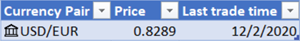
For example, Price represents the exchange rate for the currency pair, Last Trade Time represents the time the exchange rate was quoted.

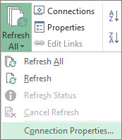
Once you have all the currency data that you want, you can use it in formulas or calculations. To ensure your data is up to date, you can go to Data > Refresh All to get an updated quote.

Caution: Currency information is provided «as-is» and may be delayed. Therefore, this data should not be used for trading purposes or advice. See About our data sources for more information.

Источник

Exchanging Data with Excel FilesпѓЃ

This is a follow up to AIMMS Excel Library — AXLL . The вЂAIMMS Excel Library (AXLL)вЂ™ lets you exchange data between AIMMS and Excel files (.xls and .xlsx) without having Excel installed on that computer. This is very useful when deploying applications using AIMMS PRO as it is typically installed on a terminal server where a copy of Microsoft Office is not available.

In this article, we show you which functions available in axll:: namespace to use depending on the format of the data in your Excel file.

Reading your Excel File in AIMMSпѓЃ

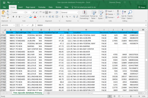
I needed some geographical information about the US for an application I was building. The information was easy to find online. I downloaded the file below, titled free-zipcode-database-Primary.xlsx . It provided the zip code, State, Latitude and Longitude columns I needed.

Next, I created a procedure in my AIMMS project, called ReadFromExcel . In the procedure, first I would like to have AIMMS point to the file so I can read it. Here is the code:

I used a String Parameter WorkBookName to take the file name. The code in the if statement is to avoid opening the workbook again if it is already opened. If it was already opened, I would just select it by calling axll::SelectWorkBook function; otherwise,I would open the file by the axll::OpenWorkBook function.

The next thing is to use axll::SelectSheet to set the sheet I am going to use.

Then I use axll::ReadSet function to read value for set sZipCode .

The first argument, axll::ReadSet::SetReference , is the set name. The second argument, axll::ReadSet::SetRange , is the range in Excel. The third argument, axll::ReadSet::ExtendSuperSets , is telling AIMMS to extend this setвЂ™s super set when the elements read in this Excel are not part of the super set.

Adding ParametersпѓЃ

Next, I want to make sure I can read the following data in two dimensional parameters Coordinates(z,iLonLat) , by using axll::ReadTable .

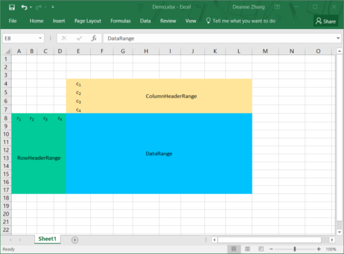
The first argument, IdentifierReference , is the name of the parameter. The second argument, RowHeaderRange , is the range for first index z , which is represented as row range «A2:A42523» in Excel. The third argument, ColumnHeaderRange , is the range for second index iLonLat , which is represented as column range «F1:G1» in Excel. The forth argument, DataRange , is the range for the actual data.

In case you have an identifier with more dimensions, RowHeaderRange is the range where the starting indices reside, and ColumnHeaderRange , is the range where the ending indices reside. For example, identifier MyValue(r1, r2, r3, r4,c1,c2,c3,c4) has 8 indices, and the data in Excel looks like this:

Then the axll::ReadTable statement will be:

Continuing with the zip code example. I then use axll::ReadSet to read in data for set sState .

And axll::ReadList to read in data ZipCodeState(z) , which holds the state name that each zip code belongs to.

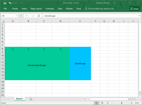
axll::ReadList is designed for reading in data which is represented as lists in Excel. So it is only with RowHeaderRange . The following Excel Sheet is an example with «A8:D17» as RowHeaderRange and «E8:E17» as DataRange.

At this point, everything I need to use in my model is in there, so I use axll::CloseWorkBook to close the workbook.

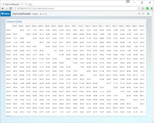
With the data I just imported from Excel, I can do further analyses. For example, I can calculate the distance between zip codes based on the latitude and longitude, and show it in AIMMS WebUI.

Similarly, you can use the AIMMSXLLibrary to write to Excel. You can see the comments in the library for further reference.

Edit this page to fix an error or add an improvement in a pull request
Create an issue to suggest an improvement to this page

Product

Create a topic if there’s something you don’t like about this feature
Propose functionality by submitting a feature request

Support

Not what you where looking for? Search the docs

Источник

Transfer of data from one Excel table to another one

A table in Excel is a complex array with set of parameters. It can consist of values, text cells, formulas and be formatted in various ways (cells can have a certain alignment, color, text direction, special notes, etc.).

When you copy a table, sometimes you do not have to transfer all of its elements, but only some of its. Consider how this can be done.

The past special

It is very convenient to carry out the transfer of the data in the table using the past special. It allows you to select only those parameters that we need when copying. Let’s consider an example.

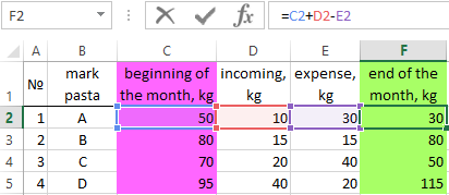
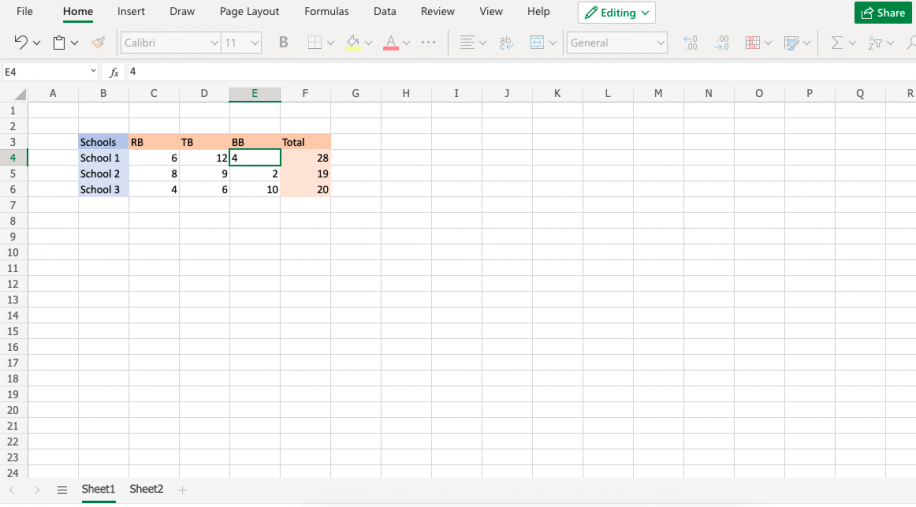
We have the table with the indicators for the presence of macaroni of certain brands in the warehouse of the store. It is clearly visible, how many kilograms were at the beginning of the month, how much of them were bought and sold, and also the balance at the end of the month. Two important columns are highlighted in different colors. The balance at the end of the month is calculated by the elementary formula.

We will try to use the PAST SPECIAL command and copy all the data.

First we select the existing table, right click the menu and click on COPY.

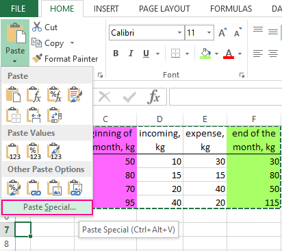
In the free cell, we call the menu again with the right button and press the PAST SPECIAL.

If we leave everything as is by default and just click OK, the table will be inserted completely, with all its parameters.

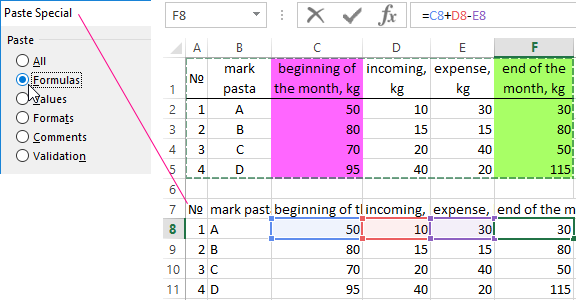
Let’s try to experiment. In the PAST SPECIAL we choose another item, for example, FORMULAS. We have already received an unformatted table, but with working formulas.

Now we will insert not the formulas, but only the VALUES of the results of calculations.

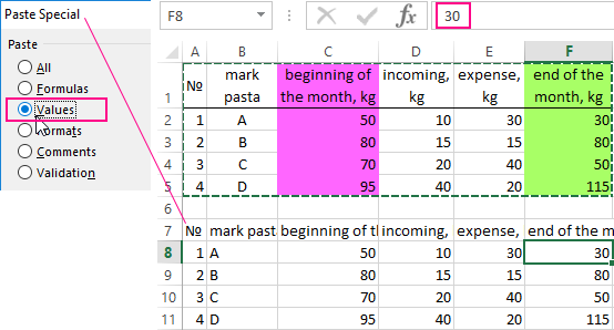
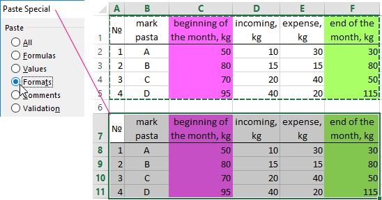
That a new table with values to get the appearance similar to the sample, you need to select it and insert the FORMATS using a special insert.

Now let’s try to choose the item WITHOUT FRAME. We got the full table, but only without the allocated borders.

The wholesome advice! To migrate the format along with the size of the columns, you need to select not the range of the source table, but the entire columns (in this case, the A: F range) before the copying.

Similarly, you can experiment with each item of the PAST SPECIAL to see clearly how it works.

Transfer of data to another sheet

Transferring data to other worksheets in the Excel workbook allows you to link multiple tables. This is convenient because when you replace a value on one sheet, the values change on all the others. When creating annual reports, this is an indispensable thing.

Consider how this works. For a start we rename Excel sheets in months. Then, with the helping of the PAST SPECIAL that we already know, we move the table to February and remove the values from the three columns:

At the beginning of the month.
The incoming.
The expense.

The column «At the end of the month» is given by the formula, so when you delete values from the previous columns, it is automatically reset to zero.

We will transfer to the data on the remainder of macaroni of each brand from January to February. This is done in a couple of clicks.

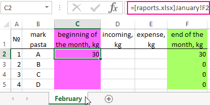
On the FEBRUARY sheet we place the cursor in the cell, indicating the amount of macaroni of grade A at the beginning of the month. You can see the picture above — this will be cell D3.
We put in this cell to the sign EQUAL.
Go to the JANUARY sheet and click on the cell showing the amount of macaroni of grade A at the end of the month (in this case it is cell F2).

We get the following: in the cell C2 the formula was formed, which sends us to the cell F2 of the JANUARY sheet. Stretch the formula down to know the amount of macaroni of each brand at the beginning of February.

Similarly, you can transfer the data to all months and get to the visual annual report.

Data transfer to another file

Similarly, you can transfer data from one file to another one. This book in our example is called EXCEL. Create another one and name it EXAMPLE.

Note. You can create new Excel files even in different folders. The program will automatically search for the specified book, regardless of which folder and on what drive of the computer it is located.

We copy in the book EXAMPLE to the table using the same PAST SPECIAL and again delete the values from the three columns. We will perform the same actions as in the previous paragraph, but we will not go to another sheet, but to another book only.

We have received to the new formula, which shows that the cell refers to the book EXCEL. And we see that the cell =[raports.xlsx]January!F2 looks like =[raports.xlsx]January!$F$2, i. e. it is fixed. And if we want to stretch to the formula in other brands of macaroni, first you need to remove the dollar badges for removing to the commit.

Now you know how to correctly transfer data from tables within one sheet, from one sheet to another, and from one file to another one.

Источник

Exchange rate in Excel

With Office 365, you can insert Exchange rate in your worksheets

The version of Excel in Office 365 allows you to collect the exchange rate of currencies of the current day.

Add Exchange Rate

The Office 365 version provides a great new feature ; Data Type. You just have to fill geographic data or financial data and Excel connects to a database to add values to the original one.

If you want to add financial data to the name of a stock holder or to return the exchange rate between 2 currencies, you just have to write your value in cells and then Click on the button Data > Stocks. You can use any separator ; space, dash, slash, pipe, .

What are the details behind the link

Once your have linked 2 currency to the Data Type tool, you can visualized all the informations in relationship between the 2 currencies by clicking on the icon

As you can see, behind a single connection between 2 currencies, you can return a lot of informations.

Return the last Exchange rate

What is amazing with Data Type, it’s the simplicity to return one of the data linked. To do that, you can click on the little rectangle in order to open the list of data you can add.

Or you can write a formula with a reference to the cell with the icon and then you press dot. Like that, you can also visualise all the information linked. Double-click or press Tab to select the option you want.

In both situation, the formula is

Copy the dotted formula (beware of the format)

Like all the formulas in Excel, you can easily drag-and-drop the fill-handle to copy the formula.

But in this situation, you must take care of the currency format. Of course, when you copy the formula, you copy also the format of the original cell.

But you can force the each format by selecting the option Update Format.

Источник

Обмен данными
через буфер

Обмен
данными через буфер производится для
всех приложений Windows.
Информация заносится в буфер по команде
Правка/Копировать.
Находящиеся в буфере данные в Excel
могут
вставляться
в другой рабочий лист, другую рабочую
книгу. Можно таблицу
Excel
вставить и в другое приложение
Windows,
например текстовый
редактор Word.
В этом случае после копирования данных
в буфер обмена нужно переключиться (или
загрузить) в редактор
Word,
задать команду Правка/Вставка.
Данные скопируются
в виде таблицы Word.

Динамический
обмен данными DDE

Динамический
обмен данными (Dynamic
Data
Exchange
— DDE)
позволяет установить постоянную связь
по обмену данными
между двумя программами Windows,
например,
Excel
с текстовым редактором Word.
Обмен данными в этом случае происходит
автоматически,
т.е. при каждом изменении цифр в таблице
Excel
такое же изменение происходит и в
таблице, находящейся в текстовом
редакторе. Обмен будет происходить
только, если обе программы открыты в
среде Windows
одновременно. Для установки
такой связи надо таблицу (или фрагмент
таблицы)
Excel
скопировать в буфер обмена, переключиться
в текстовый редактор,
задать команду Правка/Специальная
вставка,
выбрать пункт
Форматированный
текст
(rtf)
и включить опцию Связать.
Если
вместо изображения таблицы в документе
показывается строка
символов в фигурных скобках, следует
задать команду Сервис/Опции
и во вкладке Просмотр
сбросить переключатель Коды
полей.
Excel
может выступать и как импортер,
например,
текста из редактора
Word.
В этом случае текст Word
копируется в буфер обмена,
затем нужно переключиться (или загрузить)
в Excel,
задать команду Правка/Вставка/Специальная
вставка
и включить опцию
Связать.
Текст вставляется в виде объекта.
Аналогичным образом
можно вставить диаграмму Excel
на слайд
PowerPoint.

Связь
и внедрение объектов OLE

Функция
связи и внедрения объектов (Object
Linking
And
Embedding
— OLE)
позволяет организовать динамический
обмен данными,
с помощью объектов. Для установки такой
связи таблица
(или фрагмент таблицы) Excel
копируется в буфер обмена, затем нужно
переключиться в текстовый редактор,
установить курсор
в нужное место задать команду
Вставка/Объект,
вкладку Создать
новый,
в поле Тип
объекта
выбрать строку Лист
Microsoft
Excel.
После этого в документ будет вставлена
пустая таблица Excel.
Выделить начальную ячейку таблицы,
задать команду Правка/Вставить,
чтобы перенести данные из буфера обмена
в новую
таблицу. Вставленную таблицу Excel
можно редактировать в состоянии, когда
она обрамлена штриховой
рамкой. Чтобы
продолжить
работу с текстом, достаточно щелкнуть
мышью в области
текста вне таблицы. При необходимости
повторного редактирования
таблицы нужно дважды щелкнуть внутри
нее мышью.

Задание 1

Постройте
диаграмму Образование
сотрудников.
Данные для
построения диаграммы приведены в
табл.2.

Таблица 2

Данные для построения диаграммы

	A	B	C	D
1		Магнолия	Лилия	Фиалка
2	Высшее	25	20	9
3	Среднее	28	23	20
4	ПТУ	27	58	20
5	Всего	80	101	49

Соседние файлы в предмете [НЕСОРТИРОВАННОЕ]

Источник

When you copy a table, sometimes you do not have to transfer all of its elements, but only some of its. Consider how this can be done.

The past special

It is very convenient to carry out the transfer of the data in the table using the past special. It allows you to select only those parameters that we need when copying. Let’s consider an example.

We will try to use the PAST SPECIAL command and copy all the data.

First we select the existing table, right click the menu and click on COPY.

In the free cell, we call the menu again with the right button and press the PAST SPECIAL.

If we leave everything as is by default and just click OK, the table will be inserted completely, with all its parameters.

Let’s try to experiment. In the PAST SPECIAL we choose another item, for example, FORMULAS. We have already received an unformatted table, but with working formulas.

Now we will insert not the formulas, but only the VALUES of the results of calculations.

VALUES.

That a new table with values to get the appearance similar to the sample, you need to select it and insert the FORMATS using a special insert.

Now let’s try to choose the item WITHOUT FRAME. We got the full table, but only without the allocated borders.

Similarly, you can experiment with each item of the PAST SPECIAL to see clearly how it works.

Transfer of data to another sheet

At the beginning of the month.
The incoming.
The expense.

The column «At the end of the month» is given by the formula, so when you delete values from the previous columns, it is automatically reset to zero.

We will transfer to the data on the remainder of macaroni of each brand from January to February. This is done in a couple of clicks.

On the FEBRUARY sheet we place the cursor in the cell, indicating the amount of macaroni of grade A at the beginning of the month. You can see the picture above — this will be cell D3.
We put in this cell to the sign EQUAL.
Go to the JANUARY sheet and click on the cell showing the amount of macaroni of grade A at the end of the month (in this case it is cell F2).

Similarly, you can transfer the data to all months and get to the visual annual report.

Data transfer to another file

Similarly, you can transfer data from one file to another one. This book in our example is called EXCEL. Create another one and name it EXAMPLE.

Now you know how to correctly transfer data from tables within one sheet, from one sheet to another, and from one file to another one.

Источник

Do you regularly work out of multiple Excel sheets? If so, you should know how to transfer data from one sheet to another automatically. This enormous time-saver doesn’t involve complicated formulas or add-ons, and it’s especially practical if you want to transfer specific data from one worksheet to another for reports. Below, you’ll learn two simple methods to copy data from one Excel sheet to another. These methods also link the sheets so that any changes you make to one sheet’s dataset automatically apply to the other. Finally, you’ll learn how to move data from one Excel sheet to another based on criteria by using the filter feature.

If you want to transfer data from one Google Sheet to another automatically, you can do that easily using Layer. Layer is a free add-on that allows you to share sheets or ranges of your main spreadsheet with different people. On top of that, you get to monitor and approve edits and changes made to the shared files before they’re merged back into your master file, giving you more control over your data.

Install the Layer Google Sheets Add-On today and Get Free Access to all the paid features, so you can start managing, automating, and scaling your processes on top of Google Sheets!

Two methods for automatically transferring data from one Excel worksheet to another

While there are various methods for transferring data from one Excel worksheet to another, the two simplest are the Copy and Paste Link and the Worksheet Reference methods.

How to Link Sheets in Excel?

Use Copy and Paste Link to automatically transfer data from one Excel worksheet to another

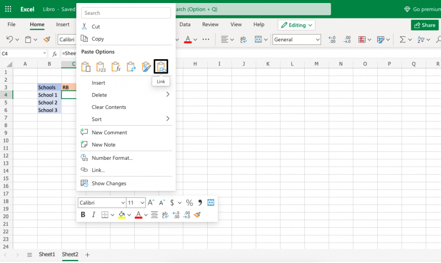
While you’re probably familiar with the standard Copy and Paste function, Excel offers multiple paste options. One of these is Link, which allows you to paste a value from another worksheet and link the pasted value to the copied value. In other words, if you change the original value you copied, the pasted value will automatically change as well.

These steps will show you how to use the Copy and Paste Link function:

1. Open two spreadsheets containing the same simple dataset.

2. In sheet 1, select a cell and type Ctrl + C / Cmd + C to copy it.

3. In sheet 2, right-click on the equivalent cell and go to the Paste > Link.

4. To prove they’re linked, return to sheet 1 and change the value in the cell you copied.

5. Finally, return to sheet 2 to see that the value has also changed.

How to VLOOKUP in Excel with Two Spreadsheets?

Sometimes our data may be spread out among different Excel sheets or workbooks. Here’s how to do VLOOKUP in Excel with two spreadsheets

Use worksheet reference to automatically transfer data from one Excel worksheet to another

This method is more manual than the Copy and Paste method but is equally simple and useful to know, just in case. The following steps will teach you how to use the worksheet reference method to transfer data from one Excel worksheet to another automatically:

1. Open two spreadsheets containing the same, simple dataset.

2. In sheet 2, double-click on a cell to the right of the dataset and type ‘=’.

3. Go to sheet 1, click any cell from the dataset, and press Enter.

You should automatically be returned to Sheet 2, where the cell previously containing ‘=’ now contains the value you chose to transfer from Sheet 1.

4. To prove they’re linked, return to Sheet 1 and change the value you chose to transfer.

Sheet 2 will automatically have changed the value to your chosen new value.

Move data from one Excel sheet to another based on criteria using the filter feature

In this example, you will learn how to filter data based on column criteria so that you keep only what you need. Then, you can copy and paste the data into a new sheet, as demonstrated in the above example.

1. Open a dataset on an Excel worksheet with filterable criteria.

2. Select the criteria column from which you want to filter and go to Data > Filter.

3. Click the small arrow beside the column header to open a drop-down menu.

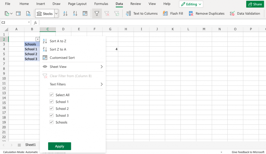
4. At the bottom of this menu, tick the box of the row(s) that you want to keep and click “Apply”.

You should now see only the data you wanted to keep.

To move this data to another sheet, follow the steps that show you how to copy and paste to automatically transfer data from one Excel worksheet to another.

Want to Boost Your Team’s Productivity and Efficiency?

Transform the way your team collaborates with Confluence, a remote-friendly workspace designed to bring knowledge and collaboration together. Say goodbye to scattered information and disjointed communication, and embrace a platform that empowers your team to accomplish more, together.

Key Features and Benefits:

Centralized Knowledge: Access your team’s collective wisdom with ease.
Collaborative Workspace: Foster engagement with flexible project tools.
Seamless Communication: Connect your entire organization effortlessly.
Preserve Ideas: Capture insights without losing them in chats or notifications.
Comprehensive Platform: Manage all content in one organized location.
Open Teamwork: Empower employees to contribute, share, and grow.
Superior Integrations: Sync with tools like Slack, Jira, Trello, and more.

Limited-Time Offer: Sign up for Confluence today and claim your forever-free plan, revolutionizing your team’s collaboration experience.

Conclusion

So, if you didn’t know before how useful it is to link and transfer data from one Excel worksheet to another automatically, you do now. With the Copy and Paste Link and worksheet reference method, you can transfer data effectively in a matter of minutes. What’s more, you’ll never have to worry about these spreadsheets again — any update in one will be automatically transferred to the other immediately. You can also move data from one Excel sheet to another based on criteria by filtering your data to transfer only what you want. This is great for transferring data for important reports, saving you lots of time from unnecessary copy and pasting, and report editing.

If you work with multiple worksheets in Excel and found this article helpful, you should also check out these related posts: How to do VLOOKUP in excel with two spreadsheets, and How to use IMPORTRANGE in Google Sheets.

Hady is Content Lead at Layer.

Hady has a passion for tech, marketing, and spreadsheets. Besides his Computer Science degree, he has vast experience in developing, launching, and scaling content marketing processes at SaaS startups.

Originally published Feb 3 2022, Updated Mar 22 2023

Источник

Excel for Microsoft 365 Excel for Microsoft 365 for Mac Excel for the web More…Less

Note: Currency pairs are only available to Microsoft 365 accounts (Worldwide Multi-Tenant clients.)

Use the Currencies data type to calculate exchange rates

Enter the currency pair in a cell using this format: From Currency / To Currency with the ISO currency codes.

For example, enter «USD/EUR» to get the exchange rate from one United States Dollar to Euros.
Select the cells and then select Insert > Table. Although creating a table isn’t required, it’ll make inserting data from the data type much easier later.
With the cells still selected, go to the Data tab and select the Currencies data type.

If Excel finds a match between the currency pair and our data provider, your text will convert to a data type and you’ll see the Currencies icon in the cell.

Note: If you see   in the cell instead of the Currencies icon, then Excel is having difficulty matching the text with data. Correct any mistakes and press Enter to try again. Or, select the icon to open the Data Selector where you can search for a currency pair or specify the data you need.
To extract more information from the Currencies data type, select one or more converted cells and select the Insert Data button that appears or press Ctrl/Cmd+Shift+F5.
You’ll see a list of all the fields available to choose from. Select the fields to add a new column of data.

For example, Price represents the exchange rate for the currency pair, Last Trade Time represents the time the exchange rate was quoted.
Once you have all the currency data that you want, you can use it in formulas or calculations. To ensure your data is up to date, you can go to Data > Refresh All to get an updated quote.

Caution: Currency information is provided «as-is» and may be delayed. Therefore, this data should not be used for trading purposes or advice. See About our data sources for more information.

Methods To Transfer Data From One Excel Workbook To Another

There are many different ways to transfer data from one Excel workbook to another and they are as follows:

Method #1: Automatically Update One Excel Worksheet From Another Sheet

In MS Excel workbook, we can easily update the data by linking one worksheet to another. This link is known as a dynamic formula that transfers data from one Excel workbook to another automatically.

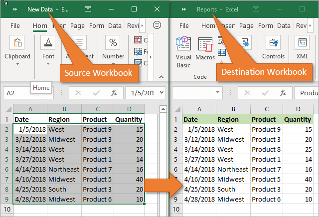
One Excel workbook is called the source worksheet, where this link carries the worksheet data automatically, and the other workbook is called the destination worksheet in which it automatically updates the worksheet data and contains the link formula.

The following are the two different points to link the Excel workbook data for the automatic updates.

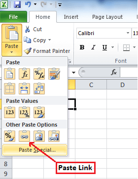
1) With the use of Copy and Paste option

In the source worksheet, select and copy the data that you want to link in another worksheet
Now in the destination worksheet, Paste the data where you have linked the cell source worksheet
After that choose the Paste Link menu from the Other Paste Options in the Excel workbook

Save all your work from the source worksheet before closing it

2) Manually enter the formula

Open your destination worksheet, tap to the cell that is having a link formula and put an equal sign (=) across it
Now go to the source sheet and tap to the cell which is having data. press Enter from your keyboard and save your tasks.

Note- Always remember one thing that the format of the source worksheet and the destination worksheet both are the same.

Method #2: Update Excel Spreadsheet With Data From Another Spreadsheet

To update Excel spreadsheets with data from another spreadsheet, just follow the points given below which will be applicable for the Excel version 2019, 2016, 2013, 2010, 2007.

At first, go to the Data menu
Select Refresh All option

Here you have to see that when or how the connection is refreshed
Now click on any cell that contains the connected data
Again in the Data menu, click on the arrow which is next to Refresh All option and select Connection Properties

After that in the Usage menu, set the options that you want to change
On the Usage tab, set any options you want to change.

Note – If the size of the Excel data workbook is large, then I will recommend checking the Enable background refresh menu on a regular basis.

Method #3: How To Copy Data From One Cell To Another In Excel Automatically

To copy data from one cell to another in Excel, just go through the following points given below:

First, open the source worksheet and the destination worksheet.
In the source worksheet, navigate to the sheet that you want to move or copy
Now, click on the Home menu and choose the Format option
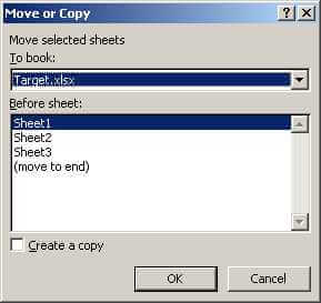
Then, select the Move Or Copy Sheet from the Organize Sheets part
After that, again in the Home menu choose the Format option in the cells group
Here in the Move Or Copy dialog option, select the target sheet and Excel will only display the open worksheets in the list

Else, if you want to copy the worksheet instead of moving, then kindly make a copy of the Excel workbook before

Lastly, select the OK button to copy or move the targeted Excel spreadsheet.

Method #4: How To Copy Data From One Sheet To Another In Excel Using Formula

You can copy data from one sheet to another in Excel using formula. Here are the steps to be followed:

For copy and paste the Excel cell in the present Excel worksheet, as for example; copy cell A1 to D5, you can just select the destination cell D5, then enter =A1 and press the Enter key to get the A1 value.
For copying and pasting cells from one worksheet to another worksheet such as copy cell A1 of Sheet1 to D5 of Sheet2, please select the cell D5 in Sheet2, then enter =Sheet1!A1 and press the Enter key to obtain the value.

Method #5: Copy Data From One Excel Sheet To Another Using Macros

With the help of macros, you can copy data from one worksheet to another but before this here are some important tips that you must take care of:

You should keep the file extension correctly in your Excel workbook.
It’s not necessary that your spreadsheet should be macro enable for doing the task.
The code that you choose can also be stored in a different worksheet.
As the codes already specify the details, so there is no need to activate the Excel workbook or cells first.
Thus, given below is the code for performing this task.

Sub OpenWorkbook()
‘Open a workbook
‘Open method requires full file path to be referenced.
Workbooks.Open “C:UsersusernameDocumentsNew Data.xlsx”

‘Open method has additional parameters
‘Workbooks.Open(FileName, UpdateLinks, ReadOnly, Format, Password, WriteResPassword, IgnoreReadOnlyRecommended, Origin, Delimiter, Editable, Notify, Converter, AddToMru, Local, CorruptLoad)

End Sub

Sub CloseWorkbook()
‘Close a workbook
Workbooks(“New Data.xlsx”).Close SaveChanges:=True
‘Close method has additional parameters
‘Workbooks.Close(SaveChanges, Filename, RouteWorkbook)

End Sub

Conclusion:

Well, I tried my level best to provide the best possible ways to transfer data from one Excel worksheet to another automatically. So from now on, you don’t have to worry about how to copy data from one cell to another in Excel automatically.

I hope you are satisfied with the above methods provided to you about Excel worksheet update.

Thus, make proper use of them and in the future also if you want to know about this, you can take the help of the specified solutions.

Priyanka is an entrepreneur & content marketing expert. She writes tech blogs and has expertise in MS Office, Excel, and other tech subjects. Her distinctive art of presenting tech information in the easy-to-understand language is very impressive. When not writing, she loves unplanned travels.

Источник

With Office 365, you can insert Exchange rate in your worksheets

The version of Excel in Office 365 allows you to collect the exchange rate of currencies of the current day.

Add Exchange Rate

The Office 365 version provides a great new feature ; Data Type. You just have to fill geographic data or financial data and Excel connects to a database to add values to the original one.

What are the details behind the link

Once your have linked 2 currency to the Data Type tool, you can visualized all the informations in relationship between the 2 currencies by clicking on the icon

As you can see, behind a single connection between 2 currencies, you can return a lot of informations.

Return the last Exchange rate

What is amazing with Data Type, it’s the simplicity to return one of the data linked. To do that, you can click on the little rectangle in order to open the list of data you can add.

In both situation, the formula is

=D2.Price

Copy the dotted formula (beware of the format)

Like all the formulas in Excel, you can easily drag-and-drop the fill-handle to copy the formula.

But in this situation, you must take care of the currency format. Of course, when you copy the formula, you copy also the format of the original cell.

But you can force the each format by selecting the option Update Format.

Источник

Download PC Repair Tool to quickly find & fix Windows errors automatically

Microsoft Excel is quite powerful in what it can be used for. If you’re one of the many folks who use Excel for financial data where exchange rates are concerned, you need to learn how to get currency exchange rates from within Excel. Before moving forward, we should point out that this feature is only available to Microsoft Office 365 subscribers. This wasn’t the case before, but Microsoft decided to change its policy, so now is time if you haven’t yet subscribed. Additionally, if you are subscribed the feature will work just as fine with Excel on the Web.

Allowing the Microsoft Excel app to showcase currency exchange data is easier than one might have originally expected. This is mostly due to the built-in tools Excel has provided, tools that are only found in the Office 365 version.

Open Microsoft Excel
Add the currency pairs
Apply the Data Type for each currency
Add the Exchange Data to cells
Get current Exchange Data

1] Open Microsoft Excel

To begin, you must first launch into Microsoft Excel 365 if you haven’t already. This is the easier part, as one might expect.

Look for the Microsoft Excel shortcut icon on your computer.
Click on it to open the app right away without delays.

2] Add the currency pairs

Once the Excel app is up and running, you must open a blank workbook and then add the currency pairs you want to work with. Click on New Workbook to open a new spreadsheet in order to move forward.

From within the new spreadsheet, select one of the top cells.
Add titles for each Cell. For example, add these titles in cells A, B, C, etc.
The first heading, you can call it Currency.
Under the Currency heading, you can add your favorite pairs.
Ensure each pair is added in the following format: (USD/JPY).

3] Apply the Data Type for each currency

You’ll now be required to add a Data Type for each currency pair you’ve added to the spreadsheet. This is important in order for the calculations to work.

Click on the cell where you entered the relevant currency pair.
The next step, then, is to click on the Data tab.
From the Data Types box, select Currencies.
The selected cell should now be updated, demonstrating you’ve employed the Currencies type.

Bear in mind that if you come across a question mark instead of the icon related to the Currencies data, then it means Microsoft Excel is having issues with matching the data you’ve added. Please double-check to see if the ISO codes for the currency type are correct.

4] Add the Exchange Data to cells

We now need to select the Exchange Data in a bid to populate the cells with relevant information.

Select one of the currency pair cells.
Click on the Insert Data icon that appears at the right.
You should now be looking at a list of information.
Select any to insert them into the spreadsheet.

Note that whenever data is selected, it appears in the cell immediately to the right of the symbol cell. As more data is added, they will continue appearing to the further right.

5] Get current Exchange Data

At some point you will want to have the most current details in your spreadsheet, so what to do? Well, it makes no sense to update each cell one after the other, so let us discuss an easier way to get things done.

Return to the Data tab by selecting it.
Navigate to the Queries & Connections section.
Finally, click on Refresh All, then select Refresh from the dropdown menu.

Doing this should effectively update all data on your spreadsheet to the latest if any are available.

Read: How to convert currencies in Excel

Can you get live exchange rates in Excel?

If you’re not interested in getting live exchange rates by going through the hard way, well, luck is on your side because an easier option exists. We suggest downloading a free add-in from the official Professor Excel website.

Read: How to Display or Format Number as Currency in Excel

How do you automatically change the currency in Excel?

Changing the currency in Excel is a simple task. All you have to do is select the cell you want to format, and from there, click on the Home tab, then select Currency from the Number Format. A dropdown menu will appear, and that’s where you’ll select the currency symbols will appear. Choose the currency that you prefer and that’s it for that.

Read next: How to convert Currency and get Stock Data in Google Sheets.

Ezoic

Vamien has studied Computer Information Services and Web Design. He has over 10 years of experience in building desktop computers, fixing problems relating to Windows, and Python coding.

Источник

Get a currency exchange rate

Use the Currencies data type to calculate exchange rates

Exchanging Data with Excel FilesпѓЃ

Reading your Excel File in AIMMSпѓЃ

Adding ParametersпѓЃ

Product

Support

Transfer of data from one Excel table to another one

The past special

Transfer of data to another sheet

Data transfer to another file

Exchange rate in Excel

With Office 365, you can insert Exchange rate in your worksheets

Add Exchange Rate

What are the details behind the link

Return the last Exchange rate

Copy the dotted formula (beware of the format)

Задание 1

Данные для построения диаграммы

The past special

Transfer of data to another sheet

Data transfer to another file

Two methods for automatically transferring data from one Excel worksheet to another

How to Link Sheets in Excel?

Use Copy and Paste Link to automatically transfer data from one Excel worksheet to another

How to VLOOKUP in Excel with Two Spreadsheets?

Use worksheet reference to automatically transfer data from one Excel worksheet to another

Move data from one Excel sheet to another based on criteria using the filter feature

Want to Boost Your Team’s Productivity and Efficiency?

Conclusion

Use the Currencies data type to calculate exchange rates

See also

Need more help?

Want more options?

Practical Scenario

Methods To Transfer Data From One Excel Workbook To Another

Method #1: Automatically Update One Excel Worksheet From Another Sheet

Method #2: Update Excel Spreadsheet With Data From Another Spreadsheet

Method #3: How To Copy Data From One Cell To Another In Excel Automatically

Method #4: How To Copy Data From One Sheet To Another In Excel Using Formula

Method #5: Copy Data From One Excel Sheet To Another Using Macros

Recommended Solution: MS Excel Repair & Recovery Tool

Steps to Utilize MS Excel Repair & Recovery Tool:

Conclusion:

With Office 365, you can insert Exchange rate in your worksheets

Add Exchange Rate

What are the details behind the link

Return the last Exchange rate

Copy the dotted formula (beware of the format)

1] Open Microsoft Excel

2] Add the currency pairs

3] Apply the Data Type for each currency

4] Add the Exchange Data to cells

5] Get current Exchange Data

Can you get live exchange rates in Excel?

How do you automatically change the currency in Excel?