
Excel for Microsoft 365 Excel for Microsoft 365 for Mac Excel for the web More…Less
With the Currencies data type you can easily get and compare exchange rates from around the world. In this article, you’ll learn how to enter currency pairs, convert them into a data type, and extract more information for robust data.
Note: Currency pairs are only available to Microsoft 365 accounts (Worldwide Multi-Tenant clients.)
Use the Currencies data type to calculate exchange rates
-
Enter the currency pair in a cell using this format: From Currency / To Currency with the ISO currency codes.
For example, enter «USD/EUR» to get the exchange rate from one United States Dollar to Euros.
-
Select the cells and then select Insert > Table. Although creating a table isn’t required, it’ll make inserting data from the data type much easier later.
-
With the cells still selected, go to the Data tab and select the Currencies data type.
If Excel finds a match between the currency pair and our data provider, your text will convert to a data type and you’ll see the Currencies icon
 in the cell.
Note: If you see
in the cell instead of the Currencies icon, then Excel is having difficulty matching the text with data. Correct any mistakes and press Enter to try again. Or, select the icon to open the Data Selector where you can search for a currency pair or specify the data you need. -
To extract more information from the Currencies data type, select one or more converted cells and select the Insert Data button
that appears or press Ctrl/Cmd+Shift+F5. -
You’ll see a list of all the fields available to choose from. Select the fields to add a new column of data.
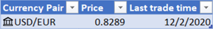
For example, Price represents the exchange rate for the currency pair, Last Trade Time represents the time the exchange rate was quoted.
-
Once you have all the currency data that you want, you can use it in formulas or calculations. To ensure your data is up to date, you can go to Data > Refresh All to get an updated quote.
Caution: Currency information is provided «as-is» and may be delayed. Therefore, this data should not be used for trading purposes or advice. See About our data sources for more information.
See also
Stocks and geography data types
How to write formulas that reference data types
FIELDVALUE function
#FIELD! error
Need more help?
With Office 365, you can insert Exchange rate in your worksheets
The version of Excel in Office 365 allows you to collect the exchange rate of currencies of the current day.

Add Exchange Rate
The Office 365 version provides a great new feature ; Data Type. You just have to fill geographic data or financial data and Excel connects to a database to add values to the original one.
If you want to add financial data to the name of a stock holder or to return the exchange rate between 2 currencies, you just have to write your value in cells and then Click on the button Data > Stocks. You can use any separator ; space, dash, slash, pipe, …

What are the details behind the link
Once your have linked 2 currency to the Data Type tool, you can visualized all the informations in relationship between the 2 currencies by clicking on the icon

As you can see, behind a single connection between 2 currencies, you can return a lot of informations.
Return the last Exchange rate
What is amazing with Data Type, it’s the simplicity to return one of the data linked. To do that, you can click on the little rectangle in order to open the list of data you can add.

Or you can write a formula with a reference to the cell with the icon and then you press dot. Like that, you can also visualise all the information linked. Double-click or press Tab to select the option you want.

In both situation, the formula is
=D2.Price
Copy the dotted formula (beware of the format)
Like all the formulas in Excel, you can easily drag-and-drop the fill-handle to copy the formula.
But in this situation, you must take care of the currency format. Of course, when you copy the formula, you copy also the format of the original cell.
But you can force the each format by selecting the option Update Format.

Download PC Repair Tool to quickly find & fix Windows errors automatically
Microsoft Excel is quite powerful in what it can be used for. If you’re one of the many folks who use Excel for financial data where exchange rates are concerned, you need to learn how to get currency exchange rates from within Excel. Before moving forward, we should point out that this feature is only available to Microsoft Office 365 subscribers. This wasn’t the case before, but Microsoft decided to change its policy, so now is time if you haven’t yet subscribed. Additionally, if you are subscribed the feature will work just as fine with Excel on the Web.
Allowing the Microsoft Excel app to showcase currency exchange data is easier than one might have originally expected. This is mostly due to the built-in tools Excel has provided, tools that are only found in the Office 365 version.
- Open Microsoft Excel
- Add the currency pairs
- Apply the Data Type for each currency
- Add the Exchange Data to cells
- Get current Exchange Data
1] Open Microsoft Excel
To begin, you must first launch into Microsoft Excel 365 if you haven’t already. This is the easier part, as one might expect.
- Look for the Microsoft Excel shortcut icon on your computer.
- Click on it to open the app right away without delays.
2] Add the currency pairs
Once the Excel app is up and running, you must open a blank workbook and then add the currency pairs you want to work with. Click on New Workbook to open a new spreadsheet in order to move forward.
- From within the new spreadsheet, select one of the top cells.
- Add titles for each Cell. For example, add these titles in cells A, B, C, etc.
- The first heading, you can call it Currency.
- Under the Currency heading, you can add your favorite pairs.
- Ensure each pair is added in the following format: (USD/JPY).
3] Apply the Data Type for each currency

You’ll now be required to add a Data Type for each currency pair you’ve added to the spreadsheet. This is important in order for the calculations to work.
- Click on the cell where you entered the relevant currency pair.
- The next step, then, is to click on the Data tab.
- From the Data Types box, select Currencies.
- The selected cell should now be updated, demonstrating you’ve employed the Currencies type.
Bear in mind that if you come across a question mark instead of the icon related to the Currencies data, then it means Microsoft Excel is having issues with matching the data you’ve added. Please double-check to see if the ISO codes for the currency type are correct.
4] Add the Exchange Data to cells

We now need to select the Exchange Data in a bid to populate the cells with relevant information.
- Select one of the currency pair cells.
- Click on the Insert Data icon that appears at the right.
- You should now be looking at a list of information.
- Select any to insert them into the spreadsheet.
Note that whenever data is selected, it appears in the cell immediately to the right of the symbol cell. As more data is added, they will continue appearing to the further right.
5] Get current Exchange Data

At some point you will want to have the most current details in your spreadsheet, so what to do? Well, it makes no sense to update each cell one after the other, so let us discuss an easier way to get things done.
- Return to the Data tab by selecting it.
- Navigate to the Queries & Connections section.
- Finally, click on Refresh All, then select Refresh from the dropdown menu.
Doing this should effectively update all data on your spreadsheet to the latest if any are available.
Read: How to convert currencies in Excel
Can you get live exchange rates in Excel?
If you’re not interested in getting live exchange rates by going through the hard way, well, luck is on your side because an easier option exists. We suggest downloading a free add-in from the official Professor Excel website.
Read: How to Display or Format Number as Currency in Excel
How do you automatically change the currency in Excel?
Changing the currency in Excel is a simple task. All you have to do is select the cell you want to format, and from there, click on the Home tab, then select Currency from the Number Format. A dropdown menu will appear, and that’s where you’ll select the currency symbols will appear. Choose the currency that you prefer and that’s it for that.
Read next: How to convert Currency and get Stock Data in Google Sheets.

Vamien has studied Computer Information Services and Web Design. He has over 10 years of experience in building desktop computers, fixing problems relating to Windows, and Python coding.
Содержание
- Получить обменный курс валюты
- Использование типа данных «Валюты» для расчета обменных курсов
- Get a currency exchange rate
- Use the Currencies data type to calculate exchange rates
- Live and Historic Currency Exchange Rates in Excel
- Exchange rate in Excel
- With Office 365, you can insert Exchange rate in your worksheets
- Add Exchange Rate
- What are the details behind the link
- Return the last Exchange rate
- Copy the dotted formula (beware of the format)
- Currency exchange rate example
- Related functions
- Summary
- Generic formula
- Explanation
- Overview
- Basic currency exchange example
- Connecting the input cells
Получить обменный курс валюты
С помощью типа данных Валюты можно легко получить и сравнить обменные курсы по всему миру. В этой статье вы узнаете, как вводить пары валют, преобразовывать их в тип данных и извлекать дополнительные сведения для надежных данных.
Примечание: Валютные пары доступны только для Microsoft 365 (клиенты с несколькими клиентами по всему миру).
Использование типа данных «Валюты» для расчета обменных курсов
Введите валютную пару в ячейку, используя такой формат: Из валюты / В валюту с кодами валют ISO.
Например, введите «ДОЛЛАР/ЕВРО», чтобы получить курс обмена от одного доллара США к евро.
Выберем ячейки и выберите Вставить > таблицу. Создание таблицы не обязательно, но значительно упростит вставку данных из типа данных.
Выбрав ячейки, перейдите на вкладку Данные и выберите тип данных Валюты.
Если Excel обнаружит совпадение между валютной парой и поставщиком данных, текст преобразуется в тип данных, а в ячейке  значок Валюты.
Примечание: Если в ячейке  вместо значка Валюты, Excel затруднение при совпадении текста с данными. Исправь все ошибки и нажмите ввод, чтобы повторить попытку. Можно также выбрать значок, чтобы открыть селектор данных, в котором можно найти валютную пару или указать нужные данные.
Чтобы извлечь дополнительные сведения из типа данных Валюты, выберите одну или несколько преобразованных ячеек и нажмите кнопку Вставить данные  отобразить или нажать клавиши CTRL/CMD+SHIFT+F5.
Вы увидите список всех доступных полей. Выберите поля, чтобы добавить новый столбец данных.
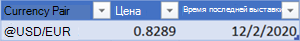
Например, «Цена» представляет обменный курс для валютной пары, а время последней сделки — время, в течение которого курс был цитироваться.
После того как у вас есть все необходимые данные о валюте, их можно использовать в формулахи вычислениях. Чтобы убедиться, что данные обновлены, перейдите в> Обновить все, чтобы получить обновленную кавычка.
Внимание: Сведения о валюте предоставляются «как есть» и могут быть задержаны. Поэтому эти данные не следует использовать в целях торговли или советов. Дополнительные сведения см. всведениях об источниках данных.
Источник
Get a currency exchange rate
With the Currencies data type you can easily get and compare exchange rates from around the world. In this article, you’ll learn how to enter currency pairs, convert them into a data type, and extract more information for robust data.
Note: Currency pairs are only available to Microsoft 365 accounts (Worldwide Multi-Tenant clients.)
Use the Currencies data type to calculate exchange rates
Enter the currency pair in a cell using this format: From Currency / To Currency with the ISO currency codes.
For example, enter «USD/EUR» to get the exchange rate from one United States Dollar to Euros.
Select the cells and then select Insert > Table. Although creating a table isn’t required, it’ll make inserting data from the data type much easier later.
With the cells still selected, go to the Data tab and select the Currencies data type.
If Excel finds a match between the currency pair and our data provider, your text will convert to a data type and you’ll see the Currencies icon  in the cell.
Note: If you see  in the cell instead of the Currencies icon, then Excel is having difficulty matching the text with data. Correct any mistakes and press Enter to try again. Or, select the icon to open the Data Selector where you can search for a currency pair or specify the data you need.
To extract more information from the Currencies data type, select one or more converted cells and select the Insert Data button  that appears or press Ctrl/Cmd+Shift+F5.
You’ll see a list of all the fields available to choose from. Select the fields to add a new column of data.
For example, Price represents the exchange rate for the currency pair, Last Trade Time represents the time the exchange rate was quoted.
Once you have all the currency data that you want, you can use it in formulas or calculations. To ensure your data is up to date, you can go to Data > Refresh All to get an updated quote.
Caution: Currency information is provided «as-is» and may be delayed. Therefore, this data should not be used for trading purposes or advice. See About our data sources for more information.
Источник
Live and Historic Currency Exchange Rates in Excel
Excel Price Feed is ideal for populating your Excel spreadsheet with live currency exchange rates.
Introduction
If you run an international business that deals in a variety of currencies or are simply trying to work out how much you spent on holiday then you have no doubt spent time updating a spreadsheet with the latest exchange rates.
This usually means looking up the rate on a website then copying/pasting the rate into a cell in your sheet. This process is repeated for each currency, and is repeated again whenever you want to update the fx rates (the fx market is open 24 hours a day).
There is an easier way, you can use the Excel Price Feed Add-in to automatically retrieve live exchange rates into Excel cells.
You set up the formula once and then each time you refresh your spreadsheet the latest live exchange rates are retrieved and the rate in the cell is updated.
Live Exchange Rates Example
After installing the Add-in you now have access to 100+ new Excel formulas, including the one below which will retrieve the live Euro / US Dollar (EUR/USD) exchange rate from Yahoo Finance:
This formula uses currency code of the exchange rate you require, the convention for Yahoo Finance is the currency pair code followed by «=X».
If you don’t know the currency code then you can use the search screen on the Configuration Pane, accessed from the button on the toolbar.
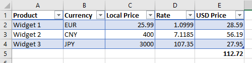
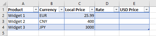
For this example we will start with a table of widgets that we are sourcing from 3 different countries which are priced in 3 different currencies:
To populate the USD price column we just need to provide the live exchange rate to the «Rate» column, for example here we can see the EPF.Yahoo.Price formula used for the Euro widget in the Rate cell:
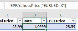
We repeat this formula for the next two rows, we now have the dollar price for each widget and can calculate a dollar total for all 3 widgets:
Any time you wish to update the exchange rates, simply press the «Refresh Sheet» button on the Excel Price Feed toolbar, no more copying/pasting exchange rates!
Historic Exchange Rates
Excel Price Feed also provides the ability to retrieve historic exchange rates into Excel cells. This is achieved using the EPF.Yahoo.Historic.Close formula.
For example, this formula will retrieve the Euro/US Dollar (EURUSD) exchange rate as it was on 1 January 2019:
Summary
We hope this tutorial really helps you save time building Excel spreadsheets that need live currency exchange rates.
Discover the power of Excel Price Feed with 80+ new Excel formulas for live, historic and fundamental data in your spreadsheet. Click the button below to request an Activation Code for your free 10 day trial:
Источник
Exchange rate in Excel
With Office 365, you can insert Exchange rate in your worksheets
The version of Excel in Office 365 allows you to collect the exchange rate of currencies of the current day.
Add Exchange Rate
The Office 365 version provides a great new feature ; Data Type. You just have to fill geographic data or financial data and Excel connects to a database to add values to the original one.
If you want to add financial data to the name of a stock holder or to return the exchange rate between 2 currencies, you just have to write your value in cells and then Click on the button Data > Stocks. You can use any separator ; space, dash, slash, pipe, .
What are the details behind the link
Once your have linked 2 currency to the Data Type tool, you can visualized all the informations in relationship between the 2 currencies by clicking on the icon
As you can see, behind a single connection between 2 currencies, you can return a lot of informations.
Return the last Exchange rate
What is amazing with Data Type, it’s the simplicity to return one of the data linked. To do that, you can click on the little rectangle in order to open the list of data you can add.
Or you can write a formula with a reference to the cell with the icon and then you press dot. Like that, you can also visualise all the information linked. Double-click or press Tab to select the option you want.
In both situation, the formula is
Copy the dotted formula (beware of the format)
Like all the formulas in Excel, you can easily drag-and-drop the fill-handle to copy the formula.
But in this situation, you must take care of the currency format. Of course, when you copy the formula, you copy also the format of the original cell.
But you can force the each format by selecting the option Update Format.
Источник
Currency exchange rate example

Summary
To get historical currency exchange rates over time, you can use the STOCKHISTORY function. In the example shown, the formula in cell B4 is:
The result is the monthly exchange rate for the USD > EUR currency pair shown in cells F5 and F6. Note that STOCKHISTORY returns an array of values that spill onto the worksheet into multiple cells. The STOCKHISTORY is only available in Excel 365.
Generic formula
Explanation
In this example, the goal is to get monthly currency exchange rates for a given currency pair (i.e. USD > EUR, USD > GBP, CAD > JPY, etc.). Currency abbreviations are entered in cells F5 and F6, and the start and end dates are entered in cells F7 and F8. If any of these four inputs are changed, the results seen in columns B and C will update dynamically. This can be done with the STOCKHISTORY function, whose purpose is to retrieve historical information for a financial instrument over time.
Overview
Although the name suggests otherwise, the STOCKHISTORY function can work with a variety of financial instruments, including bonds, index funds, mutual funds, bonds, and currency pairs. To work with currency exchange rates, STOCKHISTORY requires a currency pair entered as text.
STOCKHISTORY takes up to 11 arguments, most of which are optional. The syntax for the first 4 arguments looks like this:
Stock is a unique key for the instrument being retrieved, entered as a text value. For currency exchange rates, stock will be a currency pair like «USD:CAD». Start_date and end_date are Excel dates that define the time period being requested. Interval is the time interval – daily, weekly, or monthly. For a more complete description of all arguments and properties, see our STOCKHISTORY function page.
Basic currency exchange example
To get exchange rates for a given currency pair with STOCKHISTORY, enter the two 3-letter codes separated by a colon (:) as the stock argument. For example, to get the currency exchange rate between the US Dollar («USD») and the Euro («EUR») for the months of January 2021 through March 2021, you can use STOCKHISTORY like this:
In this example, the stock argument is the text value «USD:EUR», start_date is «1-Jan-2021», end_date is «1-Mar-2021». The interval argument specifies the time period to use between prices. The options are daily (0), weekly (1), or monthly (2). In this case, we want a monthly interval, so we provide 2. The result is an array with three months of rates:
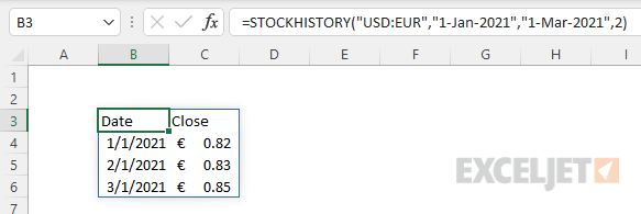
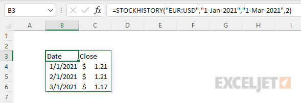
To reverse the direction of the exchange, just swap the order of the currency pairs:
Returns exchange rates in the opposite direction:
Note: in general, it’s safer to use the DATE function to enter dates in other formulas because it eliminates the risk of a text value being misinterpreted on other systems with different locale settings, but in this case dates are entered as text to keep things simple.
Connecting the input cells
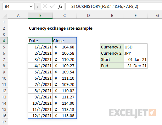
To connect the basic formula above with the input cells in the example, shown, we need to substitute cell references for the hardcoded values. The final formula in cell B4 is:
Notice we assemble the stock argument by concatenating the currency symbols in cells F5 and F6 together, separated by a colon:
The result is fully dynamic. If any of these four inputs are changed, STOCKHISTORY will immediately return a new set of exchange rates. In the screen below, currency 1 has been set to «USD» (US Dollar) and currency 2 has been set to «JPY» (Japanese Yen):
The STOCKHISTORY function automatically sets the currency symbol as needed.
Note: when interval is set to monthly (2) as in this example, the STOCKHISTORY function will return the last available exchange rate in a given month.
Источник
Here’s a ‘no fuss, no muss’ way to grab the latest exchange rates and use them in Excel. No need to lookup a rate and type it in, let Excel do all that work for you.
You might expect Excel to do this out of the box. After all, Microsoft has been banging on about Internet integration for years and their main rival, Google, has an exchange rate function in their spreadsheets (see GoogleFinance() ).
 Real Time Excel
 Real Time Excel
Real-Time Excel – get live stock, fund and bond prices, currency rates and more includes working spreadsheets for this tip and many other examples of getting live information into Excel. Buy and get it today (just a few minutes from now)
Tip: If you have Excel 365 there’s a much easier way see Exchange Rate support in Excel 365
There are many places on the web which supply exchange rate information in a computer readable format. Excel can grab that data and put it into cells for the worksheet. For this article, we set some limitations:
- No VBA code or addons. This removes security concerns or hassles. Our example uses a simple .xlsx worksheet.
- Simple system that’s easy to explore and understand.
- Free access to the exchange rate information
- Xrates in XML format (which Excel understands).
Microsoft once provided a connection to their MSN data source but that’s been dropped.
For our examples, we’ll use data from FloatRates.com because their XML data format is simple and uncomplicated compared to others. The web link is simple, needs no changing parameters and no registration.
For the latest US Dollar exchange rates go to http://www.floatrates.com/daily/usd.xml this is an XML data feed which looks like a web page via a XML style sheet. Choose ‘View Source’ in your browser to see the underlying data which is what Excel will copy into a worksheet.

FloatRates.com web page (left) and source page as XML (right)
FloatRates.com also has exchange rates with other currencies as a base.
Canada: http://www.floatrates.com/daily/cad.xml
UK: http://www.floatrates.com/daily/gbp.xml
Euro: http://www.floatrates.com/daily/eur.xml
Australia: http://www.floatrates.com/daily/aud.xml
New Zealand: http://www.floatrates.com/daily/nzd.xml
For the full list go to http://www.floatrates.com/feeds.html
Data Connection
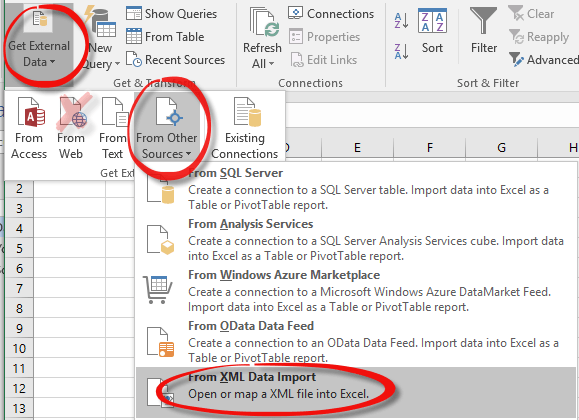
The standard recommendation for web data importing is Data | Get External Data | From Web which works for web pages with tables (the <TABLE> tag) but that doesn’t work if the XML data is changed with a style sheet.
So, we dig a little deeper to Get External Data | From Other Sources | From XML data import. This tells Excel to ignore the style sheet formatting and use the XML data only.
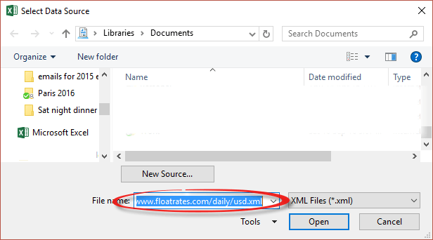
Paste the web link (complete with http:// or preferably https:// prefix) in the Select Data Source dialog. See above for a list of options.
Excel will warn if there’s no XML schema available, that’s OK, let Excel create one for you. An XML schema is the structure of the XML data feed which, officially, should always be supplied. In practice, many XML feeds don’t have a schema because it’s obvious from the feed itself.

Next, tell Excel where to put the data, most likely a New worksheet.
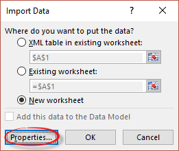
Before clicking OK, check out the Properties.

Name: make sure the Query name is self-explanatory
Refresh Control: Make the refresh rate suitable to the data feed. In this case the data is only updated every 12 hours, so there’s no point in refreshing every hour (the default).
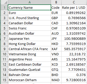
Now there’s a worksheet with 92 current conversions from US Dollar to international currencies in your worksheet.
Use Vlookup() to grab the exchange rate you want for your calculation.

Note: Vlookup requires the source data to be sorted on the column you’ll be using for the lookup. Do that from the Data | Sort tab.

You have to re-sort the list after each time the data is refreshed. Real-Time Excel – get live stock prices, currency rates and more shows how to get around that Excel limitation.
Check your calculation!
It’s too easy to get an exchange rate ‘turned around’. Even experts can get the Buy and Sell rates for a currency confused. Here’s a snippet of the ‘USD dollar’ rate feed.

These rates apply if you have US dollars and what you’ll get if you buy the other currency. For example, if you have USD$1 you’ll get 0.89 Euro, 77 UK pence or $1.311 Aussie dollars.
The common mistake is the multiply the rate given when you want to buy (convert into) the base currency. That’s wrong and will give you very misleading answers.
Reverse xrate: if you want to convert from other currencies to the base currency (US dollars in this case) divide the rate into 1. ( = 1/rate ). Do that by making a ‘parallel’ column that converts the rate.

Now you can convert from and to the base currency. Just make sure you choose the correct column/rate!
Double check: check your worksheet logic by doing tests against one of the many currency conversion web sites.
That’s just the basics of online data import into Excel for currency conversions. Real-Time Excel – get live stock prices, currency rates and more has useful extra info you should get with the currency data. Also, other online data that Excel can grab.
Excel Price Feed is ideal for populating your Excel spreadsheet with live currency exchange rates.
Introduction
If you run an international business that deals in a variety of currencies or are simply trying to work out how much you spent on holiday then you have no doubt spent time updating a spreadsheet with the latest exchange rates.
This usually means looking up the rate on a website then copying/pasting the rate into a cell in your sheet. This process is repeated for each currency, and is repeated again whenever you want to update the fx rates (the fx market is open 24 hours a day).
There is an easier way, you can use the Excel Price Feed Add-in to automatically retrieve live exchange rates into Excel cells.
You set up the formula once and then each time you refresh your spreadsheet the latest live exchange rates are retrieved and the rate in the cell is updated.
Live Exchange Rates Example
After installing the Add-in you now have access to 100+ new Excel formulas, including the one below which will retrieve the live Euro / US Dollar (EUR/USD) exchange rate from Yahoo Finance:
=EPF.Yahoo.Price("EURUSD=X")
This formula uses currency code of the exchange rate you require, the convention for Yahoo Finance is the currency pair code followed by «=X».
If you don’t know the currency code then you can use the search screen on the Configuration Pane, accessed from the button on the toolbar.
For this example we will start with a table of widgets that we are sourcing from 3 different countries which are priced in 3 different currencies:
To populate the USD price column we just need to provide the live exchange rate to the «Rate» column, for example here we can see the EPF.Yahoo.Price formula used for the Euro widget in the Rate cell:
We repeat this formula for the next two rows, we now have the dollar price for each widget and can calculate a dollar total for all 3 widgets:
Any time you wish to update the exchange rates, simply press the «Refresh Sheet» button on the Excel Price Feed toolbar, no more copying/pasting exchange rates!
Historic Exchange Rates
Excel Price Feed also provides the ability to retrieve historic exchange rates into Excel cells. This is achieved using the EPF.Yahoo.Historic.Close formula.
For example, this formula will retrieve the Euro/US Dollar (EURUSD) exchange rate as it was on 1 January 2019:
=EPF.Yahoo.Historic.Close("EURUSD=X","1 Jan 2019")
Summary
We hope this tutorial really helps you save time building Excel spreadsheets that need live currency exchange rates.
Discover the power of Excel Price Feed with 80+ new Excel formulas for live, historic and fundamental data in your spreadsheet. Click the button below to request an Activation Code for your free 10 day trial:
Try it FREE for 10 days
In this example, the goal is to get monthly currency exchange rates for a given currency pair (i.e. USD > EUR, USD > GBP, CAD > JPY, etc.). Currency abbreviations are entered in cells F5 and F6, and the start and end dates are entered in cells F7 and F8. If any of these four inputs are changed, the results seen in columns B and C will update dynamically. This can be done with the STOCKHISTORY function, whose purpose is to retrieve historical information for a financial instrument over time.
Overview
Although the name suggests otherwise, the STOCKHISTORY function can work with a variety of financial instruments, including bonds, index funds, mutual funds, bonds, and currency pairs. To work with currency exchange rates, STOCKHISTORY requires a currency pair entered as text.
STOCKHISTORY takes up to 11 arguments, most of which are optional. The syntax for the first 4 arguments looks like this:
=STOCKHISTORY(stock,start_date,[end_date],[interval])
Stock is a unique key for the instrument being retrieved, entered as a text value. For currency exchange rates, stock will be a currency pair like «USD:CAD». Start_date and end_date are Excel dates that define the time period being requested. Interval is the time interval – daily, weekly, or monthly. For a more complete description of all arguments and properties, see our STOCKHISTORY function page.
Basic currency exchange example
To get exchange rates for a given currency pair with STOCKHISTORY, enter the two 3-letter codes separated by a colon (:) as the stock argument. For example, to get the currency exchange rate between the US Dollar («USD») and the Euro («EUR») for the months of January 2021 through March 2021, you can use STOCKHISTORY like this:
=STOCKHISTORY("USD:EUR","1-Jan-2021","1-Mar-2021",2)
In this example, the stock argument is the text value «USD:EUR», start_date is «1-Jan-2021», end_date is «1-Mar-2021». The interval argument specifies the time period to use between prices. The options are daily (0), weekly (1), or monthly (2). In this case, we want a monthly interval, so we provide 2. The result is an array with three months of rates:

To reverse the direction of the exchange, just swap the order of the currency pairs:
=STOCKHISTORY("EUR:USD","1-Jan-2021","1-Mar-2021",2)
Returns exchange rates in the opposite direction:

Note: in general, it’s safer to use the DATE function to enter dates in other formulas because it eliminates the risk of a text value being misinterpreted on other systems with different locale settings, but in this case dates are entered as text to keep things simple.
Connecting the input cells
To connect the basic formula above with the input cells in the example, shown, we need to substitute cell references for the hardcoded values. The final formula in cell B4 is:
=STOCKHISTORY(F5&":"&F6,F7,F8,2)
Notice we assemble the stock argument by concatenating the currency symbols in cells F5 and F6 together, separated by a colon:
F5&":"&F6 // returns ""USD:EUR"
The result is fully dynamic. If any of these four inputs are changed, STOCKHISTORY will immediately return a new set of exchange rates. In the screen below, currency 1 has been set to «USD» (US Dollar) and currency 2 has been set to «JPY» (Japanese Yen):

The STOCKHISTORY function automatically sets the currency symbol as needed.
Note: when interval is set to monthly (2) as in this example, the STOCKHISTORY function will return the last available exchange rate in a given month.

If you use Microsoft Excel for financial data where exchange rates are part of what you need, check out the Currencies data type. This gives you various exchange details that you can include in your spreadsheet.
You can obtain the last trade time, high and low, change percent, and more by entering a pair of ISO currency codes. Then, simply select the details you want to include and refresh the data as needed.
Note: As of May 2022, the feature is only available to Microsoft 365 subscribers. You can use the feature in Excel for Microsoft 365 on Windows and Mac as well as Excel for the web.
Enter the Currency Pairs
You’ll enter a pair of currencies using the ISO codes as: From Currency / To Currency. You can use a colon instead of a slash if you prefer, but Excel will convert it to a slash when you apply the data type.
RELATED: How to Convert Currency in Microsoft Excel
So, to obtain the exchange rate and details from U.S. dollars to Euros, you would enter: USD/EUR. Or, for Australian dollars to U.S. dollars you would enter: AUD/USD.

Once you add the pair(s) you want to use, you’ll apply the data type and select the details to display.
Apply the Currencies Data Type
Select the cell where you entered the currency pair. Go to the Data tab and choose “Currencies” in the Data Types box.
You’ll see your cell update to display the data type icon on the left, indicating you’ve applied the Currencies type.
Note: If you see a question mark instead of the Currencies data type icon, that means Excel is having trouble matching the data you entered. Double-check the ISO codes for the currency types or click the question mark for more help.
Select the Exchange Data
With the currency pair cell selected, click the Insert Data icon that appears on the right. You’ll see a list of information that you can select from and insert into your sheet.
By default, the data you pick appears in the cell immediately to the right of the cell containing the currency pair. As you select more details to add, each one displays to the right as well.
Note this caution from Microsoft when obtaining currency exchange rates using this Excel feature:
Currency information is provided “as-is” and may be delayed. Therefore, this data should not be used for trading purposes or advice.
Refresh the Exchange Data
To have the most current details in your sheet, you can refresh the data as needed. For all items, go to the Data tab and click “Refresh All” in the Queries & Connections section of the ribbon.
For a particular item, select it and use the Refresh All drop-down arrow to pick “Refresh.”
If you like using the Currencies data type feature, take a look at how to use the Geography and Stocks options or even create your own data type!
READ NEXT
- › HoloLens Now Has Windows 11 and Incredible 3D Ink Features
- › BLUETTI Slashed Hundreds off Its Best Power Stations for Easter Sale
- › Google Chrome Is Getting Faster
- › The New NVIDIA GeForce RTX 4070 Is Like an RTX 3080 for $599
- › How to Adjust and Change Discord Fonts
- › This New Google TV Streaming Device Costs Just $20
How-To Geek is where you turn when you want experts to explain technology. Since we launched in 2006, our articles have been read billions of times. Want to know more?

You can use Microsoft Excel not only to create regular spreadsheets. There is a way to make your currency converter. In other words, you can make your currency exchange rates if you need to show some financial data report, for example. A special Currencies function is used for this purpose in Microsoft Excel.
You can get the time of the last trade, highs and lows, percent change, and more by entering a couple of ISO currency codes. Then simply select the details you want to include and update the data as needed.
You should also know that the Currencies option is only available now to Microsoft 365 subscribers. Well, there’s nothing complicated about getting currency exchange rates in Microsoft Excel. Here’s how you can do it.
How to use the Currencies option to calculate exchange rates in Microsoft Excel
With the Currencies option, you can easily obtain and compare currency rates from around the world. So, follow these steps:
- First of all, enter a currency pair in the cell using this format: From Currency / To Currency with ISO currency codes. For example, enter “USD/EUR” to get the exchange rate of one U.S. dollar to one euro.
- Then highlight the cells and click “Insert”.
- Select “Table” from the list. Although creating a table is optional, it will make it much easier to insert data from the data type later on.
- After that, go to the “Data” tab and select the “Currencies” data type.
If the program finds a match between the currency pair and the data provider, your text will be converted to the data type and the Currencies icon for the stock will appear in the cell.
If you see a question mark instead of a Currencies icon in a cell, Excel is having trouble matching text to data. Fix any errors and press Enter to try again. Alternatively, select the icon to open the Data Selector, where you can find the currency pair or specify the data you want.
Next, you need to:
- Select one or more converted cells and choose the Insert Data button that appears, or press Ctrl/Cmd + Shift + F5.
- You will see a list of all available fields to select from. Choose the fields to add a new data column.
Now, you can use it in formulas or calculations. To make sure your data is up to date, you can click “Data” and select “Refresh All” to get an updated quote. If you want to update only one pair you can select it and click “Refresh”.
How to convert currencies in Microsoft Excel
There is a way to convert currencies in Microsoft Excel without using a currency converter. To do this, you only need to use one formula.
To convert one currency to another, you must use 3 columns on the Excel sheet. The first column is for the target currency, the second is for the exchange rate, and the third is for the converted currency.
The formulas look like this: [Location of the first cell]*$[Column for exchange rate]$[Row for exchange rate]
Where [Location of the first cell] is the location of the first cell in the column of cells with the monetary values of the target currency. [Column for exchange rate] and [Row for exchange rate] are the column letter and row numbers for the cell in which the exchange rate is mentioned.
Essentially, this formula is designed to simply multiply the target currency by the exchange rate.
Read Also:
- How to add today’s date in Microsoft Excel
- How to switch the X and Y-axis in Microsoft Excel
- How to build a bubble chart in Microsoft Excel
How to calculate the exchange rate between two currencies in Microsoft Excel
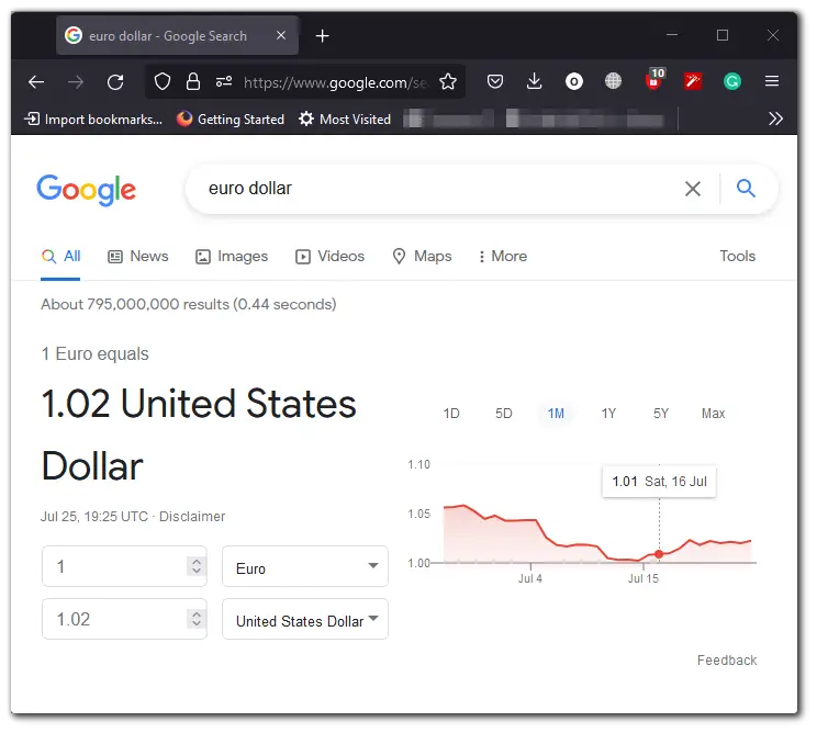
Finding an exchange rate between two currencies is easy. Open Google and simply type in the abbreviations of the two currencies you want to compare. It will automatically display the exchange rate per unit of the first currency.
Suppose you have a column of values in dollars with values located from cell A2 to A6. You need the corresponding values in euros in column C, starting in cells C2 through C6.
- Write the exchange rate in cell B2.
- Now write the formula = A2*$B$2 in cell C2 and press Enter.
- Click anywhere outside of cell C2 and then again on cell C2 to highlight the Fill button.
- Pull down cell C2 to cell C6, and it will display all the euro values in sequence.
Adding a unit of currency is one of the difficulties of this method. Nevertheless, it’s better than buying a special tool specifically for this.