Of all the functions introduced in Excel 2007, 2010, and 2013, my personal favorite is SUMIFS. The SUMIFS function performs multiple condition summing. The function is designed with AND logic, but, there are several techniques that allow us to use OR logic instead. This post explores a few of them.
Note: if your version of Excel has the FILTER function, check out this post as well.
Objective
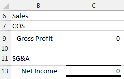
Let’s be clear about our objective by taking a look at a worksheet. Let’s assume we are trying to generate a little report based on data exported from an accounting system. We would like to write formulas to populate the report shown below.
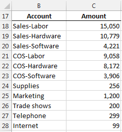
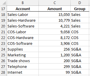
We want to populate the report by aggregating the values from the exported accounting data, shown below.
Since the SUMIFS function is designed with AND logic, the following formula wouldn’t work to populate the report’s sales value:
=SUMIFS($C$18:$C$28,
$B$18:$B$28,"Sales-Labor",
$B$18:$B$28,"Sales-Hardware",
$B$18:$B$28,"Sales-Software")
The formula wouldn’t work because there are no rows where the account is equal to Sales-Labor AND equal to Sales-Hardware AND equal to Sales-Software. As a result, the formula above returns zero.
Now that we have a clear idea of the situation, let’s work through several approaches.
SUMIFS and Wildcard
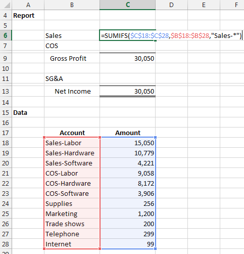
If we are lucky, there is a uniform pattern in the labels that we can use with wildcards. For example, in the data above, all of the sales accounts happen to start with “Sales-” and that makes us really lucky. We can simply use a wildcard to tell the SUMIFS function to add up any rows where the account begins with Sales- as shown in the formula below:
=SUMIFS($C$18:$C$28,$B$18:$B$28,"Sales-*")
Here it is in the report:
Note: Alternatively, we could reference the report label in the cell, and update the third argument to B6&”*”
A similar function could populate the COS report value, as follows:
=SUMIFS($C$18:$C$28,$B$18:$B$28,"COS-*")
And then we could populate the SG&A report value by adding up all of the accounts that do not have a dash, as follows:
=SUMIFS($C$18:$C$28,$B$18:$B$28,"<>*-*")
However, in practice, we are not often lucky enough to have such a pattern. So, let’s explore other options.
SUMIFS+SUMIFS
Another option is to simply string together a series of SUMIFS functions, each one designed to aggregate a specific label. For example, we could use SUMIFS to add up all rows where the account is equal to Sales-Labor, and then add to its result a SUMIFS function designed to add up all rows where account is equal to Sales-Hardware, and so on. This idea can be illustrated as follows:
=SUMIFS()+SUMIFS()+SUMIFS()
The corresponding formula to populate the sales report value is shown below.
=SUMIFS($C$18:$C$28,$B$18:$B$28,"Sales-Labor")+
SUMIFS($C$18:$C$28,$B$18:$B$28,"Sales-Hardware")+
SUMIFS($C$18:$C$28,$B$18:$B$28,"Sales-Software")
When there are only a couple of criteria values, this approach may get the job done. When there are several criteria values, we can simplify the formula and remove the redundancy by using an array criteria value argument. Let’s examine this approach now.
SUM(SUMIFS({}))
We can create a list of criteria values and include them in a single SUMIFS argument. To create a list like this, technically called an array, we simply surround it with {curly brackets}. There is one little trick to get this approach to work, but, let’s take it one step at a time.
First, let’s take a look at a formula that includes the account list in an array argument:
=SUMIFS($C$18:$C$28,$B$18:$B$28,{"Sales-Labor","Sales-Hardware","Sales-Software"})
You’ll notice that we used a SUMIFS function with a single criteria value argument. The criteria value argument is a comma-separated list surrounded by {curly braces}. This essentially tell’s the function to return the amounts for each of the listed accounts.
However, when we hit Enter, we notice that the formula only returns the sum of the first account, Sales-Labor. This brings us to our little trick. The array argument causes the formula to return three results, and since we wrote the formula in a single cell, we only see the first result. To have our cell show the sum of all three results, we simply enclose the SUMIFS function in a SUM function, as follows:
=SUM(SUMIFS($C$18:$C$28,
$B$18:$B$28,{"Sales-Labor","Sales-Hardware","Sales-Software"}))
Note: if you are familiar with array formulas, you can select three cells, then hit Ctrl+Enter to view the three results in three cells.
While each of the approaches above may achieve our objective, there is another approach that may work better for recurring-use workbooks. The concern with all of the options above is that they store the criteria values, the account names, in the cells as text strings. This prevents us from using consistent formulas within the report range. Whenever possible, we try to write consistent formulas within a range that can be filled down. We are unable to fill the above formulas because the criteria values are embedded in them. Since this makes the worksheet more difficult to maintain over time, it is often preferred to store the criteria values in cells and then reference the cells in the SUMIFS function. We can accomplish this by using a simple report group lookup table.
Report Group Lookup
Before we dig into the mechanics, let’s take a step back for a moment. Essentially, we are trying to group transaction values for reporting purposes, but, the group labels do not appear in the data. Had the accounting system exported the report group labels, our job would have been easy. The good news is that even though it didn’t, we can easily define the report groups with a simple lookup table.
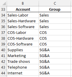
Consider the following lookup table which defines the desired report groups.
We can easily add a helper column to the data table that retrieves the proper report group. We can use our favorite lookup function to accomplish this task. For example, the following formula retrieves the report group with a VLOOKUP function:
=VLOOKUP(B18,$B$34:$C$44,2,0)
When we fill the formula down, the updated data table includes the report group, as shown below.
Now, we can populate the report’s sales value with a simple formula.
=SUMIFS($C$18:$C$28,$D$18:$D$28,B6)
We can fill this formula down throughout the report as shown below.
The consistent formulas make us very happy and the report group column makes it clear how the values flow into the report.
If you have any other techniques for using OR logic with SUMIFS, please share by posting a comment below…thanks!
Additional Resources
- Download sample file: SUMIFS with OR
- The SUMPRODUCT function can also be used to perform conditional summing with OR logic
- If you needed to use OR logic for numerous column, instead of within a single column as discussed above, be careful not to double-count rows that meet both criteria
- Excel University Volume 2 explores the SUMIFS and VLOOKUP functions in detail
Суммирование числовых значений ячеек в диапазоне с учетом нескольких условий в коде VBA Excel. Метод WorksheetFunction.SumIfs – синтаксис, параметры, примеры.
WorksheetFunction.SumIfs – это метод VBA Excel, который вычисляет сумму числовых значений в диапазоне ячеек с учетом нескольких условий (критериев).
WorksheetFunction.SumIfs (ДСумм, ДУсл_1, Усл_1, ДУсл_2, Усл_2, ..., ДУсл_14, Усл_14)
- ДСумм – диапазон суммирования, представляющий из себя часть таблицы, в ячейках которого, соответствующих условиям (критериям), суммируются значения.
- ДУсл – диапазон условия, представляющий из себя часть обрабатываемой таблицы, в ячейках которого ищется совпадение с условием (критерием) суммирования.
- Усл – это условие, которое применимо к диапазону, указанному перед ним, и определяющее критерий суммирования.
Первые три аргумента являются обязательными, остальные – необязательные. Всего выражение может содержать один диапазон суммирования (ДСумм) и четырнадцать пар диапазон+условие (ДУсл+Усл).
Диапазоны условий не должны повторяться – повторение приведет к ошибке. Диапазон суммирования можно один раз использовать как диапазон условия.
В параметре «Усл» метода WorksheetFunction.SumIfs можно использовать знаки подстановки:
- вопросительный знак (?) – заменяет один любой символ;
- звездочка (*) – заменяет любую последовательность символов (в том числе ни одного символа);
- тильда (~) – ставится перед вопросительным знаком или звездочкой, чтобы они обозначали сами себя.
Вычисление сумм с несколькими условиями
Таблица, которая использовалась для реализации примеров в коде VBA Excel:
| Дата | Магазин | Продавец | Выручка |
|---|---|---|---|
| 01.11.2019 | Липка | Лыкова | 20000 |
| 01.11.2019 | Берёзка | Серёжкина | 18000 |
| 01.11.2019 | Дубок | Бочкина | 23000 |
| 02.11.2019 | Липка | Лаптева | 30000 |
| 02.11.2019 | Берёзка | Брунькина | 25000 |
| 02.11.2019 | Дубок | Жёлудева | 17000 |
| 03.11.2019 | Липка | Лыкова | 24000 |
| 03.11.2019 | Берёзка | Серёжкина | 19000 |
| 03.11.2019 | Дубок | Бочкина | 35000 |
| 04.11.2019 | Липка | Лаптева | 27000 |
| 04.11.2019 | Берёзка | Брунькина | 31000 |
| 04.11.2019 | Дубок | Жёлудева | 26000 |
| 05.11.2019 | Липка | Лыкова | 16000 |
| 05.11.2019 | Берёзка | Серёжкина | 22000 |
| 05.11.2019 | Дубок | Бочкина | 33000 |
| 06.11.2019 | Липка | Лаптева | 16000 |
| 06.11.2019 | Берёзка | Брунькина | 28000 |
| 06.11.2019 | Дубок | Жёлудева | 29000 |
Если хотите повторить примеры, скопируйте эту таблицу и вставьте на рабочий лист Excel в ячейку A1. Таблица займет диапазон A1:D19.
Пример 1
Применение двух числовых условий в качестве критериев суммирования и использование диапазона суммирования в качестве диапазона условия:
|
Sub Primer1() Dim a As Double a = WorksheetFunction.SumIfs(Range(«D2:D19»), _ Range(«A2:A19»), DateValue(«03.11.2019»), _ Range(«D2:D19»), «>20000») MsgBox a End Sub |
В этом примере кода VBA Excel складываются все значения в диапазоне D2:D19, которые соответствуют дате 03.11.2019 в диапазоне A2:A19 и превышают 20000 в диапазоне D2:D19. Обратите внимание, что условие «>20000» заключено в прямые кавычки.
Диапазон D2:D19 используется одновременно как диапазон суммирования и как диапазон условия.
Столбец «Дата» в исходной таблице содержит даты в числовом формате, поэтому мы текстовое отображение нужной даты преобразовали в число: DateValue(«03.11.2019»). Если ячейкам этого столбца присвоить текстовый формат, то в условии суммирования дату необходимо будет указать как строку: «03.11.2019».
Пример 2
Использование в условиях суммирования переменных и подстановочных знаков:
|
Sub Primer2() Dim a As Double, b As String, c As String b = «>=» & CLng(DateValue(«04.11.2019»)) c = «*ина» a = WorksheetFunction.SumIfs(Range(«D2:D19»), _ Range(«A2:A19»), b, Range(«B2:B19»), «Берёзка», _ Range(«C2:C19»), c) MsgBox a End Sub |
В коде второго примера переменные в строке с методом WorksheetFunction.SumIfs можно заменить выражениями, которые присваиваются этим переменным.
Переменная «b» содержит условие, которое помогает отобрать из диапазона A2:A19 все даты, начиная с 04.11.2019 по 06.11.2019. Функция преобразования типа данных CLng необходима для того, чтобы при записи в строковую переменную дата записалась в виде числа, а не в формате «ДД.ММ.ГГГГ».
Из диапазона B2:B19 отбираются строки, содержащие текст «Берёзка».
Переменная «c» позволяет выбрать в диапазоне C2:C19 все фамилии, оканчивающиеся на «ина».
Третье условие на результаты выполнения кода примера 2 не влияет, так как фамилии всех продавцов «Берёзки» оканчиваются на «ина»: Серёжкина, Брунькина. Но вот если исключить второе условие, то к ним добавится Бочкина.
Смотрите также статьи о методах WorksheetFunction.Sum (суммирование без условия) и WorksheetFunction.SumIf (суммирование с одним условием).
Summing up cells based on specific conditions using SUMIFS is one of the most common tasks Excel users do. You may need to perform those sums using VBA when doing some parts of an automation task. In this post, we will show you how to write Excel SUMIFS in VBA with examples.
VBA SUMIFS function
SUMIFS is an Excel worksheet function. In VBA, you can access SUMIFS by its function name, prefixed by WorksheetFunction, as follows:
WorksheetFunction.SumIfs(...)Or,
Application.WorksheetFunction.SumIfs(...)When working with VBA code in Excel, you will be using the objects provided by the Excel object model. The top of the hierarchy is the Application object, and it has many properties, including the WorksheetFunction. If a worksheet function is used without an object being specified, then Application is automatically supplied as the object. So, in this case, you can safely omit the Application object qualifier to make your code shorter.
Excel VBA SUMIFS syntax and parameters
When you access SUMIFS in VBA, you’ll see the following syntax:
As you can see in the above image, SUMIFS returns Double. The last argument is [Arg29], but actually, the function has up to 255 arguments, which allows for 127 range-criteria pairs. This makes SUMIFS great for summing up values based on multiple criteria.
See the following explanation of the SUMIFS arguments.
Arguments or parameters
| Name | Required/Optional | Description |
Arg1 |
Required | sum_range. The range of cells to sum. |
Arg2, Arg3 |
Required | criteria_range1, criteria1. The pair of the first criteria range and criteria. |
[Arg4, Arg5], … |
Optional | [criteria_range2, criteria2], …Additional pairs of criteria range and criteria. |
Notice that the first pair of the criteria range and the criteria is required, while the rest are not. Thus, you can also use it for single criteria like SUMIF Excel.
Advanced filters using operators & wildcards in SUMIFS VBA
When using SUMIFS to filter cells based on certain criteria, you can use operators and wildcards for partial matching. This is part of the reason why this function is so powerful when used correctly!
Operators
Here are the operators you can use with your criteria:
- “
>” (greater than) - “
>=” (greater than or equal to) - “
<” (less than) - “
<=” (less than or equal to) - “
<>” (not equal to) - “
=” (equal to — but it’s optional to use this operator when using “is equal to” criteria)
Wildcards
Use the following wildcard characters in the criteria to help you find similar but not exact matches.
- A question mark (
?) matches any single character.
For example,Ja?ematches “Jade” and “Jane” - An asterisk (
*) matches any sequence of characters.
For example,Ja*matches “Jane”, “Jade”, “Jake”, and “James” - A tilde (
~) followed by?,*, or~matches a question mark, asterisk, or tilde.
For example, Discount~* matches “Discount*”
Knowing how to perform Excel functions in VBA can be a great benefit if you’re dealing with Excel every day. You may need to write SUMIFS in VBA as part of a bigger task. For example, every week, you need to automatically import data from multiple sources, process the data, summarize it using SUMIFS, and finally send a report in MS Word or Powerpoint.
Using VBA, you can import data from multiple external sources, clean it, and prepare it for further analysis and reporting. However, if you want an alternative to importing data without coding, take a look at Coupler.io. It’s a solution that allows you to import data from different sources such as Shopify, Jira, Airtable, etc., into Excel, Google Sheets, or BigQuery.
Now, let’s see a basic example of writing Excel SUMIFS in VBA. You can download the following file to follow along:
SumIfs – Basic example.xlsm
VBA SUMIFS: Basic example
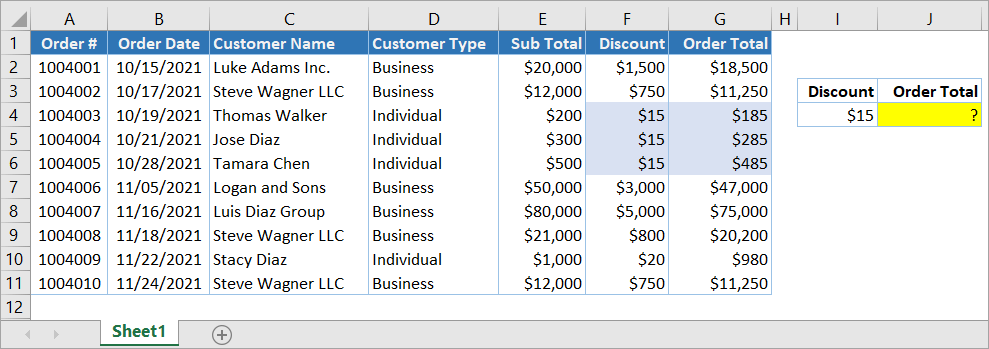
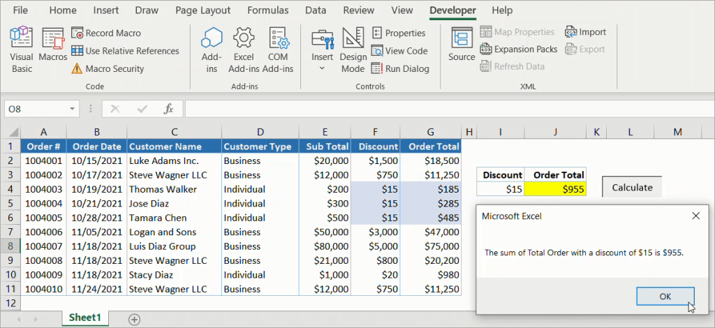
Suppose you have a workbook containing order data in Sheet1, as shown in the following screenshot. Using VBA, you want to sum the Order Total for orders with a discount based on the value in cell I4, which is $15.
If you look closely at the above screenshot, the result is expected to be $955, which results from $185+$285+$485. The following steps show you how to create a sub-procedure (macro) in VBA to get the result using SUMIFS:
- Press Alt+11 to open the Visual Basic Editor (VBE). Alternatively, you can open the VBE by clicking the Visual Basic button of the Developer tab.
- On the menu, click Insert > Module.
- In the code window, type the following procedure:
Sub SumOrderTotalByDiscount()
    Range("J4") = WorksheetFunction.SumIfs(Range("G2:G11"), Range("F2:F11"), Range("I4"))
End Sub
The code adds up the cells in range G2:G11 if the discount value in F2:F11 equals the value in I4. Then, it outputs the result in J4.
- Run the code by pressing F5.
- Check your worksheet. In cell J4, you should see
$955.
VBA SUMIFS: How to use variables
You can use variables to label the data with more descriptive names. This way, your code can be more legible and easier to understand by other people. Take a look at the following procedure that uses variables and outputs the result of SUMIFS in a message box.
Sub SumOrderTotalByDiscountUsingVariables()
    ' Declaring variables
    Dim sumRange As Range
    Dim criteriaRange As Range
    Dim criteria As Integer
    Dim result As Double

    ' Assigning values to variables
    Set sumRange = Range("G2:G11")
    Set criteriaRange = Range("F2:F11")
    criteria = Range("I4")

    ' Calculating the result using the SUMIFS function
    result = WorksheetFunction.SumIfs(sumRange, criteriaRange, criteria)

    ' Displaying the result in a message box
    MsgBox "The sum of Total Order with a discount of $" & criteria & " is $" & result & "."
End Sub
Result:
In the above SumOrderTotalByDiscountUsingVariables() code, we declared variables within the scope of the procedure. This means they can only be used in the procedure and will no longer exist once it ends. So, in this case, there’s no need to add Set variable = Nothing for each variable just before they go out of scope.
Executing SUMIFS in VBA macro using a button
Let’s say you need to build code in VBA for someone who may not be familiar with the VBE. They might not know how to run the code using the editor or even what the Macro dialog box looks like. In this case, using buttons can be very useful because even a novice will know that clicking on one typically makes something happen.
In this example, we will take the running SumOrderTotalByDiscountUsingVariables() procedure one step further by executing it on a button click.
Here are the steps:
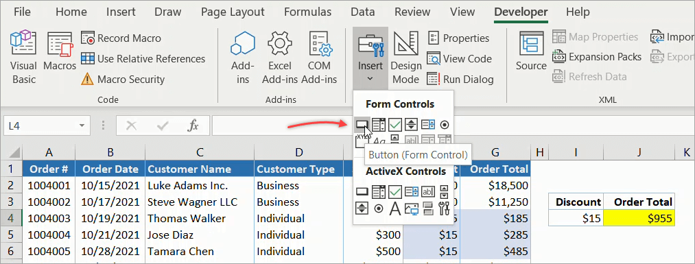
- Click the Developer tab, then click Insert > Button (Form Control).
- Click and drag anywhere on the worksheet to create a button.
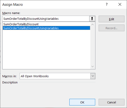
- In the “Assign Macro” dialog, select
SumOrderTotalByDiscountUsingVariables, then click OK.
- If you want, click the button’s text and edit it to “Calculate” to give it a more descriptive name.
- Now, test the button by clicking on it. You’ll see a message box appear showing the result.
More VBA SUMIFS examples: Single & multiple criteria
Now, let’s take a look at some SUMIFS examples below in VBA. We cover examples with single and multiple criteria, as well as examples with different data types for the criteria.
VBA SUMIFS less than numeric criteria
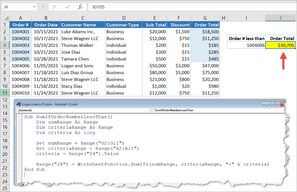
The following SUMIFS VBA code sums the Order Total for orders with numbers less than 1004006.
Sub SumIfOrderNumberLessThan()
    Dim sumRange As Range
    Dim criteriaRange As Range
    Dim criteria As Long

    Set sumRange = Range("G2:G11")
    Set criteriaRange = Range("A2:A11")
    criteria = Range("I4").Value

    Range("J4") = WorksheetFunction.SumIfs(sumRange, criteriaRange, "<" & criteria)
End Sub
We assign the criteria variable with the value from cell I4. Then, to make the “less than” filter work, we combine the “<” operator with criteria using an ampersand symbol. Also, notice that we use a Long data type for the criteria variable because Integer won’t be enough to store a 7 digit order number value.
VBA SUMIFS date criteria
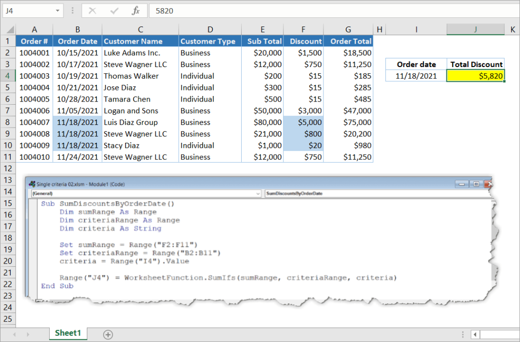
In this example, we’re summing the total discounts for orders made on 11/18/2021.
Sub SumDiscountsByOrderDate()
    Dim sumRange As Range
    Dim criteriaRange As Range
    Dim criteria As String

    Set sumRange = Range("F2:F11")
    Set criteriaRange = Range("B2:B11")
    criteria = Range("I4").Value

    Range("J4") = WorksheetFunction.SumIfs(sumRange, criteriaRange, criteria)
End Sub
We use a String data type for the criteria variable. After assigning it with the value from I4, the value will be “11/18/2021“. The “is equal to” criteria is used in the SUMIFS function, but as you can see, it’s not necessary to use the “=” operator.
VBA SUMIFS string criteria with wildcards
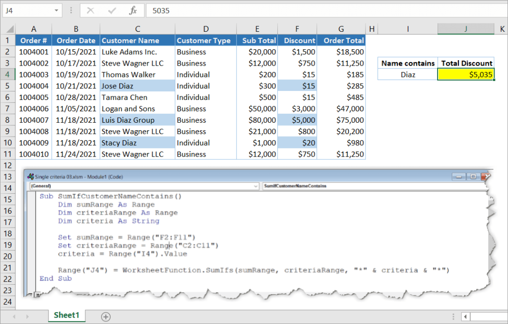
The following SUMIFS VBA sums the total discounts for orders made by customers with names containing “Diaz”.
Sub SumIfCustomerNameContains()
    Dim sumRange As Range
    Dim criteriaRange As Range
    Dim criteria As String

    Set sumRange = Range("F2:F11")
    Set criteriaRange = Range("C2:C11")
    criteria = Range("I4").Value

    Range("J4") = WorksheetFunction.SumIfs(sumRange, criteriaRange, "*" & criteria & "*")
End Sub
Notice that we use the “*” wildcard at the beginning and end of the criteria. It will match the customer names that contain “Diaz” in any position: beginning, middle, or end.
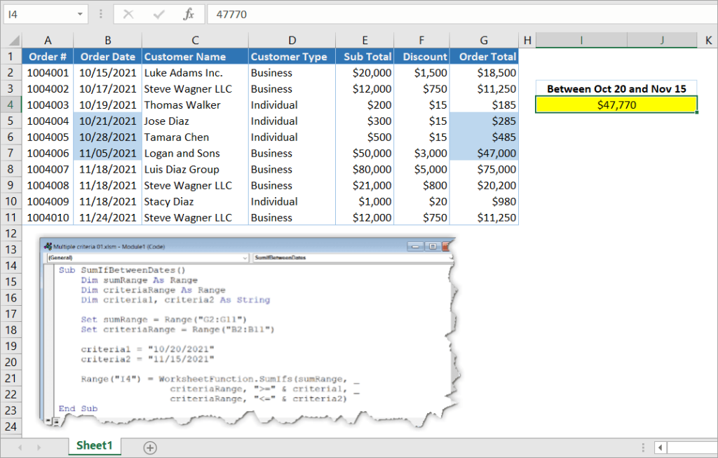
Excel VBA SUMIFS between dates
The following SUMIFS VBA procedure sums the Total Order for orders made between October 20, 2021, and November 15, 2021.
Sub SumIfBetweenDates()
    Dim sumRange As Range
    Dim criteriaRange As Range
    Dim criteria1, criteria2 As String

    Set sumRange = Range("G2:G11")
    Set criteriaRange = Range("B2:B11")

    criteria1 = "10/20/2021"
    criteria2 = "11/15/2021"

    Range("I4") = WorksheetFunction.SumIfs(sumRange, _
                    criteriaRange, ">=" & criteria1, _
                    criteriaRange, "<=" & criteria2)
End Sub
To sum values between dates, notice that we use two criteria in our SUMIFS function.
- The first criteria is for order dates that are on or after “10/20/2021”. For this, we use the “greater than or equal to” operator (>=).
- The second criteria is for order dates that are on or before “11/15/2021”. And for this, we use the “less than or equal to” operator (<=).
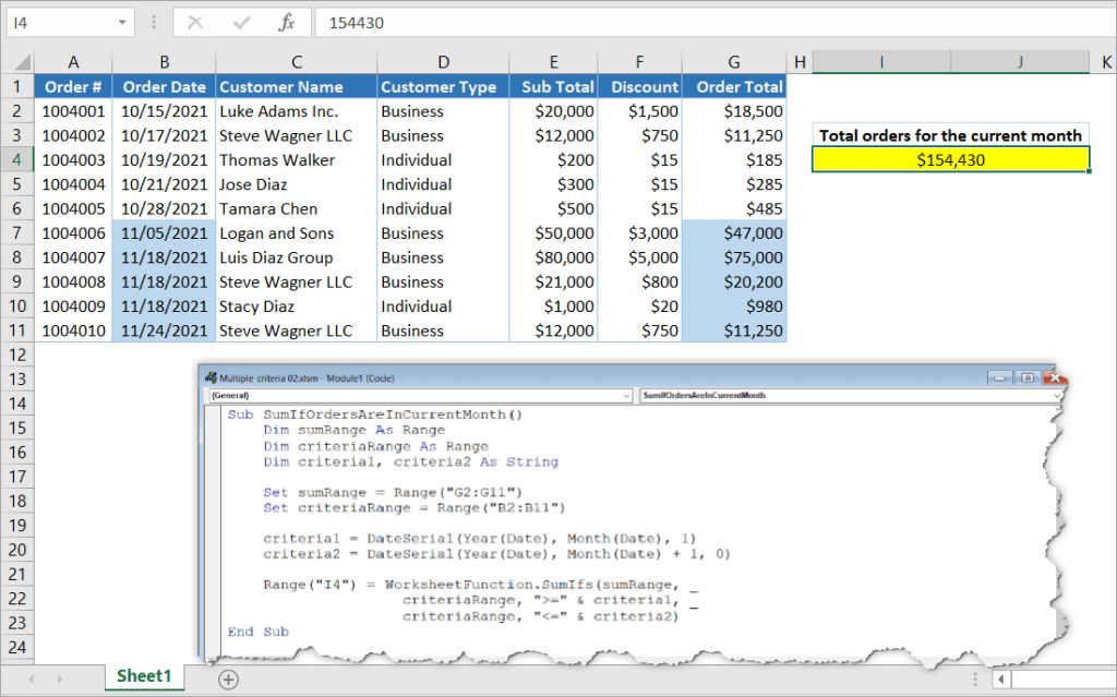
Excel VBA SUMIFS for the current month
Now, assume this month is November 2021, and you want to calculate the total discounts for orders placed this month. The solution is similar to the previous SUMIFS between dates example. You just need to change the date criteria with the start and end date of the current month.
Sub SumIfOrdersAreInCurrentMonth()
    Dim sumRange As Range
    Dim criteriaRange As Range
    Dim criteria1, criteria2 As String

    Set sumRange = Range("G2:G11")
    Set criteriaRange = Range("B2:B11")

    criteria1 = DateSerial(Year(Date), Month(Date), 1)
    criteria2 = DateSerial(Year(Date), Month(Date) + 1, 0)

    Range("I4") = WorksheetFunction.SumIfs(sumRange, _
                    criteriaRange, ">=" & criteria1, _
                    criteriaRange, "<=" & criteria2)
End Sub
In the above sub procedure, we use the following VBA functions to get the first and end date of the current month:
DateSerial(Year(Date), Month(Date), 1)— returns “11/1/2021”, which is the first day of the current month.DateSerial(Year(Date), Month(Date) + 1, 0)— returns “11/30/2021”, which is the last date of the current month.
How to combine SUMIFS with other functions in VBA
SUMIFS can be combined with other functions in VBA. For example, you can combine SUMIFS with VLOOKUP or SUM for more complex scenarios. Take a look at the following examples.
Excel VBA SUMIFS + VLOOKUP
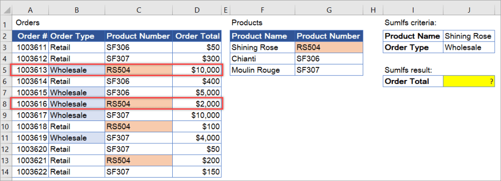
Suppose you have the following tables and want to sum up the total of wholesale orders for “Shining Rose”. You want to do the calculation using VBA and put the result in J6.
However, the Orders table does not have a Product Name, but instead it has a Product Number column. So, you need to get the Product Number of “Shining Rose” from the Products table first, then use it as one of the criteria to find the result from the Orders table using SUMIFS.
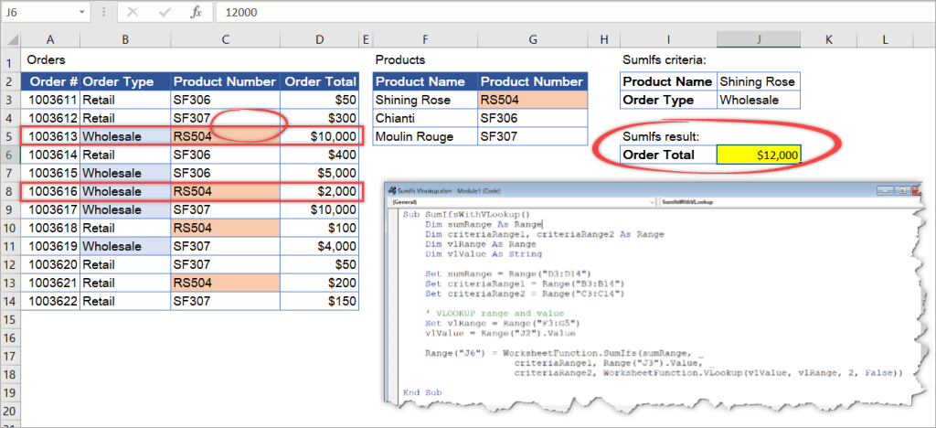
Here’s an example solution in VBA. Notice that we use WorksheetFunction.VLookup inside the SUMIFS function.
Sub SumIfsWithVLookup()
    Dim sumRange As Range
    Dim criteriaRange1, criteriaRange2 As Range
    Dim vlRange As Range
    Dim vlValue As String

    Set sumRange = Range("D3:D14")
    Set criteriaRange1 = Range("B3:B14")
    Set criteriaRange2 = Range("C3:C14")

    ' VLOOKUP range and value
    Set xRange = Range("F3:G5")
    vlValue = Range("J2").Value

    Range("J6") = WorksheetFunction.SumIfs(sumRange, _
                    criteriaRange1, Range("J3").Value, _
                    criteriaRange2, WorksheetFunction.VLookup(vlValue, vlRange, 2, False))

End Sub
Result:
Excel VBA SUMIFS + SUM across multiple sheets
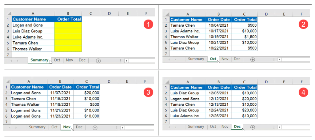
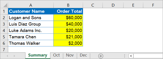
Suppose you have identical ranges in separate worksheets and want to summarize the order total by customer name in the first worksheet, as shown in the following image:
Here’s an example solution using VBA:
Sub GetOrderTotalByCustomerName()
    Dim criteria As String
    Dim result As Double
    Dim ws As Worksheet

    ' Activating the first worksheet
    Worksheets("Summary").Activate

    ' Selecting the first customer name
    Range("A2").Select

    ' Loop for each customer name
    Do Until ActiveCell.Value = ""
        criteria = ActiveCell.Value
        result = 0

        ' Loop for each worksheet other than the Summary worksheet
        For Each ws In Worksheets
            If ws.Name <> "Summary" Then

                result = WorksheetFunction.Sum(result, _
                    WorksheetFunction.SumIfs(ws.Range("C2:C6"), ws.Range("A2:A6"), criteria))
            End If
        Next ws

        ActiveCell.Offset(0, 1) = result
        ActiveCell.Offset(1, 0).Select
    Loop

End Sub
Code explanation:
- First, the code activates the Summary worksheet and selects the first customer name in cell A2.
- Then, it loops for each customer from A2, A3, … until the value in the cell is blank. Inside the loop, there’s another loop that iterates through each worksheet and performs a sum of SUMIFS.
- For each customer, their total order is output in column B.
After executing the procedure from VBE, here’s the result:
Bonus: SUMIFS VBA with array arguments for multiple OR criteria not working + solution
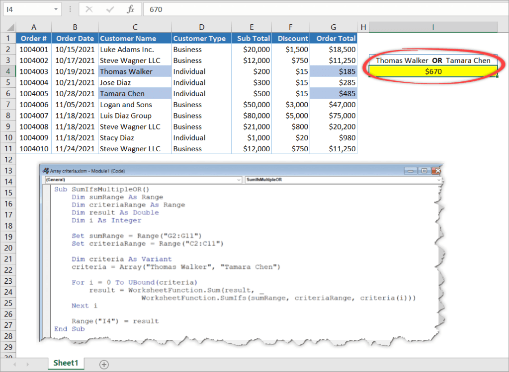
With the following table, suppose you want to sum the total order made by either Thomas Walker OR Tamara Chen.
When using a formula in a cell, you can simply use the following combination of SUM and SUMIFS with an array in its criteria argument:
=SUM(SUMIFS(G2:G11,C2:C11, {"Thomas Walker","Tamara Chen"}))
However, the following VBA code will not work:
Worksheetfunction.Sum(Worksheetfunction.SumIfs(Range("G2:G11"), Range("C2:C11"), {"Thomas Walker","Tamara Chen"}))
One of the solutions is to sum up the SUMIFS results for each criteria one by one in a loop, as follows:
Sub SumIfsMultipleOR()
    Dim sumRange As Range
    Dim criteriaRange As Range
    Dim result As Double
    Dim i As Integer

    Set sumRange = Range("G2:G11")
    Set criteriaRange = Range("C2:C11")

    Dim criteria As Variant
    criteria = Array("Thomas Walker", "Tamara Chen")

    For i = 0 To UBound(criteria)
        result = WorksheetFunction.Sum(result, _
                    WorksheetFunction.SumIfs(sumRange, criteriaRange, criteria(i)))
    Next i

    Range("I4") = result
End Sub
Result:
Wrapping up – SUMIFS VBA
The SUMIFS function is one of the most powerful functions in Excel. It can be used for summing up values based on multiple criteria, which makes it a valuable tool for data analysis and reporting. We’ve covered various examples of writing SUMIFS in VBA, including the syntax it uses, parameters, and examples of how to use it with other functions in VBA.
Interested in learning how to import data from multiple different sources into Excel with Coupler.io? Check out the Microsoft Excel integration Coupler.io offers today, as well as how this tool can help you save time and eliminate repetitive work.
-
Senior analyst programmer
Back to Blog
Focus on your business
goals while we take care of your data!
Try Coupler.io
dcuellar
New Member
- Joined
- Apr 27, 2015
- Messages
- 42
-
#1
I would like to get a SumIFs function through VBA that uses an array as criteria. This is what I have so far.
Code:
summarySht.range("O15").Value = Application.WorksheetFunction.SumIfs(dataSht.range(janCol & ":" & janCol), _
dataSht.range(GetColumnLetter(projectStatusCol) & ":" & GetColumnLetter(projectStatusCol)), projectStatus, _
dataSht.range(GetColumnLetter(programsCol) & ":" & GetColumnLetter(programsCol)), programs, _
dataSht.range(GetColumnLetter(beltDesignationCol) & ":" & GetColumnLetter(beltDesignationCol)), beltDesignation, _
dataSht.range(GetColumnLetter(benefitTypeCol) & ":" & GetColumnLetter(benefitTypeCol)), benefitType)
The variables projectStatus, programs, beltDesignation and benefitType are set up as «Dim projectStatus (0 to 3) As String», for example.
In excel the formula would allow an array within «{}». That will not work in VBA.
Any help with this would be greatly appreciated.
Last edited: Sep 1, 2016
Excel Facts
Fastest way to copy a worksheet?
Hold down the Ctrl key while dragging tab for Sheet1 to the right. Excel will make a copy of the worksheet.
RoryA
MrExcel MVP, Moderator
- Joined
- May 2, 2008
- Messages
- 40,511
- Office Version
-
- 365
- 2016
- Platform
-
- Windows
- MacOS
-
#2
Is the result supposed to be the total of every permutation of the various criteria arrays? (I ask since that wouldn’t work as a formula either)
dcuellar
New Member
- Joined
- Apr 27, 2015
- Messages
- 42
-
#3
Also, I had it set up originally to filter the different columns and then sum. My question is, will using a sumif function in VBA make the macro run faster than filter and then summing the column?
dcuellar
New Member
- Joined
- Apr 27, 2015
- Messages
- 42
-
#4
Is the result supposed to be the total of every permutation of the various criteria arrays? (I ask since that wouldn’t work as a formula either)
Yes, if I understand you correctly. So, it would be the equivalent of filtering column A for two criteria, Column B for two criteria and then summing Column C.
Last edited: Sep 1, 2016
RoryA
MrExcel MVP, Moderator
- Joined
- May 2, 2008
- Messages
- 40,511
- Office Version
-
- 365
- 2016
- Platform
-
- Windows
- MacOS
-
#5
It is probably simplest to use nested loops to loop through your three criteria arrays and accumulate the results, but I suspect a filter might be faster.
Last edited: Sep 1, 2016
Similar threads
Sometimes we need to make small amendments to formulas to make them effective.
Just like that, SUMIF OR. It’s an advanced formula that helps you to increase the flexibility of SUMIF. Yes, you can also do SUMIFS as well. But before we use it let me tell you one thing about SUMIF.
In SUMIF, you can only use one criterion and in SUMIFS, you can use more than one criterion to get a sum.
Just a thing like this. Let’s say, in SUMIFS, if you specify two different criteria, it will sum only those cells which meet both of the criteria.
Because it works with AND logic, all the criteria should meet to get a cell included. When you combine OR logic with SUMIF/SUMIFS you can sum values using two different criteria at the same time.
Without any further ado let’s learn this amazing formula.
Do We Really Need OR Logic? Any Example?
Let me show you an example where we need to add an OR logic in SUMIFS or SUMIF.
Take a look at below data table where you have a list of products with their quantity and the current status of the shipment.

In this data, you have two types of products (Faulty and Damaged) that you need to return to our vendor.
But before that, you want to calculate the total quantity of both types of products. If you go with the normal method, you have to apply SUMIF twice to get this total.
But if you use an OR condition in SUMIF then you can get the total of both of the products with just one formula.
OK, Let’s Apply OR with SUMIFS
Before we start, please download this sample file from here to follow along.
In any other cell in your worksheet where you want to calculate the total, insert the below formula and hit enter.
=SUM(SUMIFS(C2:C21,B2:B21,{"Damage","Faulty"}))
In the above formula, you have used SUMIFS but if you want to use SUMIF you can insert the below formula in the cell.
=SUM(SUMIF(B2:B21,{"Damage","Faulty"},C2:C21))By using both of the above formulas you will get 540 in the result. To cross-verify, just check the total manually.

How this formula Works
As I said, the SUMIFS function uses AND logic to sum values. But, the formula which you have used above includes an OR logic in it.
To understand this formula you have to split it into three different parts.

- The first thing is to understand that, you have used two different criteria in this formula by using the array concept. Learn more about the array from here.
- The second thing is when you specify two different values using an array, SUMIFS has to look for both of the values separately.
- The third thing is even after using an array formula, SUMIFS is not able to return the sum of both of the values in a single cell. So, that’s why you have to enclose it with the SUM function.
With the above concept, you are able to get a total for both types of products in a single cell.
It will work the same with SUMIF and SUMIFS.
And, you can also further expand your formula by specifying the product name in the second criteria in SUMIFS to get the total for a single product.
sample-file
Using Dynamic Criteria Range
In the comment section, Shay asked me about using a cell reference to add multiple criteria instead of inserting them directly into the formula.
Well, that’s a super valid question and you can do this by using a dynamic named range instead of hardcore values.
And for this, you need to do just two little amendments to your formula.
- The first is that instead of using curly brackets you need to use a named range (the best way is to use a table) of your value.
- And after that, you need to enter this formula by using Ctrl + Shift + Enter as a proper array formula.
So, now your formula will be:

Let me take you to next level of this formula. Just look at the below data table.

In this table, you have two different columns with two different kinds of statuses. Now, from this data table, you need to sum the quantity where the product is damaged return status is “No”.
That means only those Damage and Faulty products which are not been returned yet. And, the formula for this will be.
=SUM(SUMIFS(D2:D21,B2:B21,{"Damage","Faulty"},C2:C21,"No"))
sample-file
Conclusion
The best part about using the OR technique is you can add as many criteria to it. If you want to use only OR logic then it’s fine to use SUMIF. And if you want to create an OR condition and AND condition in a single formula then you can use SUMIFS for that.
You know, this is one of my favorite formula tips and I hope you found it useful.
Now tell me one thing. Have you ever used this kind of formula before? Share your views with me in the comment section, I’d love to hear from you, and please don’t forget to share this tip with your friends.

