
“It is a capital mistake to theorize before one has data”- Sir Arthur Conan Doyle
This post covers everything you need to know about using Cells and Ranges in VBA. You can read it from start to finish as it is laid out in a logical order. If you prefer you can use the table of contents below to go to a section of your choice.
Topics covered include Offset property, reading values between cells, reading values to arrays and formatting cells.
A Quick Guide to Ranges and Cells
| Function | Takes | Returns | Example | Gives |
|---|---|---|---|---|
|
Range |
cell address | multiple cells | .Range(«A1:A4») | $A$1:$A$4 |
| Cells | row, column | one cell | .Cells(1,5) | $E$1 |
| Offset | row, column | multiple cells | Range(«A1:A2») .Offset(1,2) |
$C$2:$C$3 |
| Rows | row(s) | one or more rows | .Rows(4) .Rows(«2:4») |
$4:$4 $2:$4 |
| Columns | column(s) | one or more columns | .Columns(4) .Columns(«B:D») |
$D:$D $B:$D |
Download the Code
The Webinar
If you are a member of the VBA Vault, then click on the image below to access the webinar and the associated source code.
(Note: Website members have access to the full webinar archive.)

Introduction
This is the third post dealing with the three main elements of VBA. These three elements are the Workbooks, Worksheets and Ranges/Cells. Cells are by far the most important part of Excel. Almost everything you do in Excel starts and ends with Cells.
Generally speaking, you do three main things with Cells
- Read from a cell.
- Write to a cell.
- Change the format of a cell.
Excel has a number of methods for accessing cells such as Range, Cells and Offset.These can cause confusion as they do similar things and can lead to confusion
In this post I will tackle each one, explain why you need it and when you should use it.
Let’s start with the simplest method of accessing cells – using the Range property of the worksheet.
Important Notes
I have recently updated this article so that is uses Value2.
You may be wondering what is the difference between Value, Value2 and the default:
' Value2
Range("A1").Value2 = 56

' Value
Range("A1").Value = 56

' Default uses value
Range("A1") = 56
Using Value may truncate number if the cell is formatted as currency. If you don’t use any property then the default is Value.
It is better to use Value2 as it will always return the actual cell value(see this article from Charle Williams.)
The Range Property
The worksheet has a Range property which you can use to access cells in VBA. The Range property takes the same argument that most Excel Worksheet functions take e.g. “A1”, “A3:C6” etc.
The following example shows you how to place a value in a cell using the Range property.
' https://excelmacromastery.com/
Public Sub WriteToCell()

    ' Write number to cell A1 in sheet1 of this workbook
    ThisWorkbook.Worksheets("Sheet1").Range("A1").Value2 = 67

    ' Write text to cell A2 in sheet1 of this workbook
    ThisWorkbook.Worksheets("Sheet1").Range("A2").Value2 = "John Smith"

    ' Write date to cell A3 in sheet1 of this workbook
    ThisWorkbook.Worksheets("Sheet1").Range("A3").Value2 = #11/21/2017#

End Sub
As you can see Range is a member of the worksheet which in turn is a member of the Workbook. This follows the same hierarchy as in Excel so should be easy to understand. To do something with Range you must first specify the workbook and worksheet it belongs to.
For the rest of this post I will use the code name to reference the worksheet.

The following code shows the above example using the code name of the worksheet i.e. Sheet1 instead of ThisWorkbook.Worksheets(“Sheet1”).
' https://excelmacromastery.com/
Public Sub UsingCodeName()

    ' Write number to cell A1 in sheet1 of this workbook
    Sheet1.Range("A1").Value2 = 67

    ' Write text to cell A2 in sheet1 of this workbook
    Sheet1.Range("A2").Value2 = "John Smith"

    ' Write date to cell A3 in sheet1 of this workbook
    Sheet1.Range("A3").Value2 = #11/21/2017#

End Sub
You can also write to multiple cells using the Range property
' https://excelmacromastery.com/
Public Sub WriteToMulti()

    ' Write number to a range of cells
    Sheet1.Range("A1:A10").Value2 = 67

    ' Write text to multiple ranges of cells
    Sheet1.Range("B2:B5,B7:B9").Value2 = "John Smith"

End Sub
You can download working examples of all the code from this post from the top of this article.
The Cells Property of the Worksheet
The worksheet object has another property called Cells which is very similar to range. There are two differences
- Cells returns a range of one cell only.
- Cells takes row and column as arguments.
The example below shows you how to write values to cells using both the Range and Cells property
' https://excelmacromastery.com/
Public Sub UsingCells()

    ' Write to A1
    Sheet1.Range("A1").Value2 = 10
    Sheet1.Cells(1, 1).Value2  = 10

    ' Write to A10
    Sheet1.Range("A10").Value2 = 10
    Sheet1.Cells(10, 1).Value2  = 10

    ' Write to E1
    Sheet1.Range("E1").Value2 = 10
    Sheet1.Cells(1, 5).Value2  = 10

End Sub
You may be wondering when you should use Cells and when you should use Range. Using Range is useful for accessing the same cells each time the Macro runs.
For example, if you were using a Macro to calculate a total and write it to cell A10 every time then Range would be suitable for this task.
Using the Cells property is useful if you are accessing a cell based on a number that may vary. It is easier to explain this with an example.
In the following code, we ask the user to specify the column number. Using Cells gives us the flexibility to use a variable number for the column.
' https://excelmacromastery.com/
Public Sub WriteToColumn()

    Dim UserCol As Integer

    ' Get the column number from the user
    UserCol = Application.InputBox(" Please enter the column...", Type:=1)

    ' Write text to user selected column
    Sheet1.Cells(1, UserCol).Value2 = "John Smith"

End Sub
In the above example, we are using a number for the column rather than a letter.
To use Range here would require us to convert these values to the letter/number cell reference e.g. “C1”. Using the Cells property allows us to provide a row and a column number to access a cell.
Sometimes you may want to return more than one cell using row and column numbers. The next section shows you how to do this.
Using Cells and Range together
As you have seen you can only access one cell using the Cells property. If you want to return a range of cells then you can use Cells with Ranges as follows
' https://excelmacromastery.com/
Public Sub UsingCellsWithRange()

    With Sheet1
        ' Write 5 to Range A1:A10 using Cells property
        .Range(.Cells(1, 1), .Cells(10, 1)).Value2 = 5

        ' Format Range B1:Z1 to be bold
        .Range(.Cells(1, 2), .Cells(1, 26)).Font.Bold = True

    End With

End Sub
As you can see, you provide the start and end cell of the Range. Sometimes it can be tricky to see which range you are dealing with when the value are all numbers. Range has a property called Address which displays the letter/ number cell reference of any range. This can come in very handy when you are debugging or writing code for the first time.
In the following example we print out the address of the ranges we are using:
' https://excelmacromastery.com/
Public Sub ShowRangeAddress()

    ' Note: Using underscore allows you to split up lines of code
    With Sheet1

        ' Write 5 to Range A1:A10 using Cells property
        .Range(.Cells(1, 1), .Cells(10, 1)).Value2 = 5
        Debug.Print "First address is : " _
            + .Range(.Cells(1, 1), .Cells(10, 1)).Address

        ' Format Range B1:Z1 to be bold
        .Range(.Cells(1, 2), .Cells(1, 26)).Font.Bold = True
        Debug.Print "Second address is : " _
            + .Range(.Cells(1, 2), .Cells(1, 26)).Address

    End With

End Sub
In the example I used Debug.Print to print to the Immediate Window. To view this window select View->Immediate Window(or Ctrl G)


You can download all the code for this post from the top of this article.
The Offset Property of Range
Range has a property called Offset. The term Offset refers to a count from the original position. It is used a lot in certain areas of programming. With the Offset property you can get a Range of cells the same size and a certain distance from the current range. The reason this is useful is that sometimes you may want to select a Range based on a certain condition. For example in the screenshot below there is a column for each day of the week. Given the day number(i.e. Monday=1, Tuesday=2 etc.) we need to write the value to the correct column.

We will first attempt to do this without using Offset.
' https://excelmacromastery.com/
' This sub tests with different values
Public Sub TestSelect()

    ' Monday
    SetValueSelect 1, 111.21
    ' Wednesday
    SetValueSelect 3, 456.99
    ' Friday
    SetValueSelect 5, 432.25
    ' Sunday
    SetValueSelect 7, 710.17

End Sub

' Writes the value to a column based on the day
Public Sub SetValueSelect(lDay As Long, lValue As Currency)

    Select Case lDay
        Case 1: Sheet1.Range("H3").Value2 = lValue
        Case 2: Sheet1.Range("I3").Value2 = lValue
        Case 3: Sheet1.Range("J3").Value2 = lValue
        Case 4: Sheet1.Range("K3").Value2 = lValue
        Case 5: Sheet1.Range("L3").Value2 = lValue
        Case 6: Sheet1.Range("M3").Value2 = lValue
        Case 7: Sheet1.Range("N3").Value2 = lValue
    End Select

End Sub
As you can see in the example, we need to add a line for each possible option. This is not an ideal situation. Using the Offset Property provides a much cleaner solution
' https://excelmacromastery.com/
' This sub tests with different values
Public Sub TestOffset()

    DayOffSet 1, 111.01
    DayOffSet 3, 456.99
    DayOffSet 5, 432.25
    DayOffSet 7, 710.17

End Sub

Public Sub DayOffSet(lDay As Long, lValue As Currency)

    ' We use the day value with offset specify the correct column
    Sheet1.Range("G3").Offset(, lDay).Value2 = lValue

End Sub
As you can see this solution is much better. If the number of days in increased then we do not need to add any more code. For Offset to be useful there needs to be some kind of relationship between the positions of the cells. If the Day columns in the above example were random then we could not use Offset. We would have to use the first solution.
One thing to keep in mind is that Offset retains the size of the range. So .Range(“A1:A3”).Offset(1,1) returns the range B2:B4. Below are some more examples of using Offset
' https://excelmacromastery.com/
Public Sub UsingOffset()

    ' Write to B2 - no offset
    Sheet1.Range("B2").Offset().Value2 = "Cell B2"

    ' Write to C2 - 1 column to the right
    Sheet1.Range("B2").Offset(, 1).Value2 = "Cell C2"

    ' Write to B3 - 1 row down
    Sheet1.Range("B2").Offset(1).Value2 = "Cell B3"

    ' Write to C3 - 1 column right and 1 row down
    Sheet1.Range("B2").Offset(1, 1).Value2 = "Cell C3"

    ' Write to A1 - 1 column left and 1 row up
    Sheet1.Range("B2").Offset(-1, -1).Value2 = "Cell A1"

    ' Write to range E3:G13 - 1 column right and 1 row down
    Sheet1.Range("D2:F12").Offset(1, 1).Value2 = "Cells E3:G13"

End Sub
Using the Range CurrentRegion
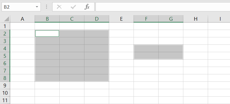
CurrentRegion returns a range of all the adjacent cells to the given range.
In the screenshot below you can see the two current regions. I have added borders to make the current regions clear.

A row or column of blank cells signifies the end of a current region.
You can manually check the CurrentRegion in Excel by selecting a range and pressing Ctrl + Shift + *.
If we take any range of cells within the border and apply CurrentRegion, we will get back the range of cells in the entire area.
For example
Range(“B3”).CurrentRegion will return the range B3:D14
Range(“D14”).CurrentRegion will return the range B3:D14
Range(“C8:C9”).CurrentRegion will return the range B3:D14
and so on
How to Use
We get the CurrentRegion as follows
' Current region will return B3:D14 from above example
Dim rg As Range
Set rg = Sheet1.Range("B3").CurrentRegion
Read Data Rows Only
Read through the range from the second row i.e.skipping the header row
' Current region will return B3:D14 from above example
Dim rg As Range
Set rg = Sheet1.Range("B3").CurrentRegion

' Start at row 2 - row after header
Dim i As Long
For i = 2 To rg.Rows.Count
    ' current row, column 1 of range
    Debug.Print rg.Cells(i, 1).Value2
Next i
Remove Header
Remove header row(i.e. first row) from the range. For example if range is A1:D4 this will return A2:D4
' Current region will return B3:D14 from above example
Dim rg As Range
Set rg = Sheet1.Range("B3").CurrentRegion

' Remove Header
Set rg = rg.Resize(rg.Rows.Count - 1).Offset(1)

' Start at row 1 as no header row
Dim i As Long
For i = 1 To rg.Rows.Count
    ' current row, column 1 of range
    Debug.Print rg.Cells(i, 1).Value2
Next i
Using Rows and Columns as Ranges
If you want to do something with an entire Row or Column you can use the Rows or Columns property of the Worksheet. They both take one parameter which is the row or column number you wish to access
' https://excelmacromastery.com/
Public Sub UseRowAndColumns()

    ' Set the font size of column B to 9
    Sheet1.Columns(2).Font.Size = 9

    ' Set the width of columns D to F
    Sheet1.Columns("D:F").ColumnWidth = 4

    ' Set the font size of row 5 to 18
    Sheet1.Rows(5).Font.Size = 18

End Sub
Using Range in place of Worksheet
You can also use Cells, Rows and Columns as part of a Range rather than part of a Worksheet. You may have a specific need to do this but otherwise I would avoid the practice. It makes the code more complex. Simple code is your friend. It reduces the possibility of errors.
The code below will set the second column of the range to bold. As the range has only two rows the entire column is considered B1:B2
' https://excelmacromastery.com/
Public Sub UseColumnsInRange()

    ' This will set B1 and B2 to be bold
    Sheet1.Range("A1:C2").Columns(2).Font.Bold = True

End Sub
You can download all the code for this post from the top of this article.
Reading Values from one Cell to another
In most of the examples so far we have written values to a cell. We do this by placing the range on the left of the equals sign and the value to place in the cell on the right. To write data from one cell to another we do the same. The destination range goes on the left and the source range goes on the right.
The following example shows you how to do this:
' https://excelmacromastery.com/
Public Sub ReadValues()

    ' Place value from B1 in A1
    Sheet1.Range("A1").Value2 = Sheet1.Range("B1").Value2

    ' Place value from B3 in sheet2 to cell A1
    Sheet1.Range("A1").Value2 = Sheet2.Range("B3").Value2

    ' Place value from B1 in cells A1 to A5
    Sheet1.Range("A1:A5").Value2 = Sheet1.Range("B1").Value2

    ' You need to use the "Value" property to read multiple cells
    Sheet1.Range("A1:A5").Value2 = Sheet1.Range("B1:B5").Value2

End Sub
As you can see from this example it is not possible to read from multiple cells. If you want to do this you can use the Copy function of Range with the Destination parameter
' https://excelmacromastery.com/
Public Sub CopyValues()

    ' Store the copy range in a variable
    Dim rgCopy As Range
    Set rgCopy = Sheet1.Range("B1:B5")

    ' Use this to copy from more than one cell
    rgCopy.Copy Destination:=Sheet1.Range("A1:A5")

    ' You can paste to multiple destinations
    rgCopy.Copy Destination:=Sheet1.Range("A1:A5,C2:C6")

End Sub
The Copy function copies everything including the format of the cells. It is the same result as manually copying and pasting a selection. You can see more about it in the Copying and Pasting Cells section.
Using the Range.Resize Method
When copying from one range to another using assignment(i.e. the equals sign), the destination range must be the same size as the source range.
Using the Resize function allows us to resize a range to a given number of rows and columns.
For example:
' https://excelmacromastery.com/
Sub ResizeExamples()

    ' Prints A1
    Debug.Print Sheet1.Range("A1").Address

    ' Prints A1:A2
    Debug.Print Sheet1.Range("A1").Resize(2, 1).Address

    ' Prints A1:A5
    Debug.Print Sheet1.Range("A1").Resize(5, 1).Address

    ' Prints A1:D1
    Debug.Print Sheet1.Range("A1").Resize(1, 4).Address

    ' Prints A1:C3
    Debug.Print Sheet1.Range("A1").Resize(3, 3).Address

End Sub
When we want to resize our destination range we can simply use the source range size.
In other words, we use the row and column count of the source range as the parameters for resizing:
' https://excelmacromastery.com/
Sub Resize()

    Dim rgSrc As Range, rgDest As Range

    ' Get all the data in the current region
    Set rgSrc = Sheet1.Range("A1").CurrentRegion

      ' Get the range destination
    Set rgDest = Sheet2.Range("A1")
    Set rgDest = rgDest.Resize(rgSrc.Rows.Count, rgSrc.Columns.Count)

    rgDest.Value2 = rgSrc.Value2

End Sub
We can do the resize in one line if we prefer:
' https://excelmacromastery.com/
Sub ResizeOneLine()

    Dim rgSrc As Range

    ' Get all the data in the current region
    Set rgSrc = Sheet1.Range("A1").CurrentRegion

    With rgSrc
        Sheet2.Range("A1").Resize(.Rows.Count, .Columns.Count).Value2 = .Value2
    End With

End Sub
Reading Values to variables
We looked at how to read from one cell to another. You can also read from a cell to a variable. A variable is used to store values while a Macro is running. You normally do this when you want to manipulate the data before writing it somewhere. The following is a simple example using a variable. As you can see the value of the item to the right of the equals is written to the item to the left of the equals.
' https://excelmacromastery.com/
Public Sub UseVariables()

    ' Create
    Dim number As Long

    ' Read number from cell
    number = Sheet1.Range("A1").Value2

    ' Add 1 to value
    number = number + 1

    ' Write new value to cell
    Sheet1.Range("A2").Value2 = number

End Sub
To read text to a variable you use a variable of type String:
' https://excelmacromastery.com/
Public Sub UseVariableText()

    ' Declare a variable of type string
    Dim text As String

    ' Read value from cell
    text = Sheet1.Range("A1").Value2

    ' Write value to cell
    Sheet1.Range("A2").Value2 = text

End Sub
You can write a variable to a range of cells. You just specify the range on the left and the value will be written to all cells in the range.
' https://excelmacromastery.com/
Public Sub VarToMulti()

    ' Read value from cell
    Sheet1.Range("A1:B10").Value2 = 66

End Sub
You cannot read from multiple cells to a variable. However you can read to an array which is a collection of variables. We will look at doing this in the next section.
How to Copy and Paste Cells
If you want to copy and paste a range of cells then you do not need to select them. This is a common error made by new VBA users.
Note: We normally use Range.Copy when we want to copy formats, formulas, validation. If we want to copy values it is not the most efficient method.
I have written a complete guide to copying data in Excel VBA here.
You can simply copy a range of cells like this:
Range("A1:B4").Copy Destination:=Range("C5")
Using this method copies everything – values, formats, formulas and so on. If you want to copy individual items you can use the PasteSpecial property of range.
It works like this
Range("A1:B4").Copy
Range("F3").PasteSpecial Paste:=xlPasteValues
Range("F3").PasteSpecial Paste:=xlPasteFormats
Range("F3").PasteSpecial Paste:=xlPasteFormulas
The following table shows a full list of all the paste types
| Paste Type |
|---|
| xlPasteAll |
| xlPasteAllExceptBorders |
| xlPasteAllMergingConditionalFormats |
| xlPasteAllUsingSourceTheme |
| xlPasteColumnWidths |
| xlPasteComments |
| xlPasteFormats |
| xlPasteFormulas |
| xlPasteFormulasAndNumberFormats |
| xlPasteValidation |
| xlPasteValues |
| xlPasteValuesAndNumberFormats |
Reading a Range of Cells to an Array
You can also copy values by assigning the value of one range to another.
Range("A3:Z3").Value2 = Range("A1:Z1").Value2
The value of range in this example is considered to be a variant array. What this means is that you can easily read from a range of cells to an array. You can also write from an array to a range of cells. If you are not familiar with arrays you can check them out in this post.
The following code shows an example of using an array with a range:
' https://excelmacromastery.com/
Public Sub ReadToArray()

    ' Create dynamic array
    Dim StudentMarks() As Variant

    ' Read 26 values into array from the first row
    StudentMarks = Range("A1:Z1").Value2

    ' Do something with array here

    ' Write the 26 values to the third row
    Range("A3:Z3").Value2 = StudentMarks

End Sub
Keep in mind that the array created by the read is a 2 dimensional array. This is because a spreadsheet stores values in two dimensions i.e. rows and columns
Going through all the cells in a Range
Sometimes you may want to go through each cell one at a time to check value.
You can do this using a For Each loop shown in the following code
' https://excelmacromastery.com/
Public Sub TraversingCells()

    ' Go through each cells in the range
    Dim rg As Range
    For Each rg In Sheet1.Range("A1:A10,A20")
        ' Print address of cells that are negative
        If rg.Value < 0 Then
            Debug.Print rg.Address + " is negative."
        End If
    Next

End Sub
You can also go through consecutive Cells using the Cells property and a standard For loop.
The standard loop is more flexible about the order you use but it is slower than a For Each loop.
' https://excelmacromastery.com/
Public Sub TraverseCells()

    ' Go through cells from A1 to A10
    Dim i As Long
    For i = 1 To 10
        ' Print address of cells that are negative
        If Range("A" & i).Value < 0 Then
            Debug.Print Range("A" & i).Address + " is negative."
        End If
    Next

    ' Go through cells in reverse i.e. from A10 to A1
    For i = 10 To 1 Step -1
        ' Print address of cells that are negative
        If Range("A" & i) < 0 Then
            Debug.Print Range("A" & i).Address + " is negative."
        End If
    Next

End Sub
Formatting Cells
Sometimes you will need to format the cells the in spreadsheet. This is actually very straightforward. The following example shows you various formatting you can add to any range of cells
' https://excelmacromastery.com/
Public Sub FormattingCells()

    With Sheet1

        ' Format the font
        .Range("A1").Font.Bold = True
        .Range("A1").Font.Underline = True
        .Range("A1").Font.Color = rgbNavy

        ' Set the number format to 2 decimal places
        .Range("B2").NumberFormat = "0.00"
        ' Set the number format to a date
        .Range("C2").NumberFormat = "dd/mm/yyyy"
        ' Set the number format to general
        .Range("C3").NumberFormat = "General"
        ' Set the number format to text
        .Range("C4").NumberFormat = "Text"

        ' Set the fill color of the cell
        .Range("B3").Interior.Color = rgbSandyBrown

        ' Format the borders
        .Range("B4").Borders.LineStyle = xlDash
        .Range("B4").Borders.Color = rgbBlueViolet

    End With

End Sub
Main Points
The following is a summary of the main points
- Range returns a range of cells
- Cells returns one cells only
- You can read from one cell to another
- You can read from a range of cells to another range of cells.
- You can read values from cells to variables and vice versa.
- You can read values from ranges to arrays and vice versa
- You can use a For Each or For loop to run through every cell in a range.
- The properties Rows and Columns allow you to access a range of cells of these types
What’s Next?
Free VBA Tutorial If you are new to VBA or you want to sharpen your existing VBA skills then why not try out the The Ultimate VBA Tutorial.
Related Training: Get full access to the Excel VBA training webinars and all the tutorials.
(NOTE: Planning to build or manage a VBA Application? Learn how to build 10 Excel VBA applications from scratch.)
Присвоение диапазона ячеек объектной переменной в VBA Excel. Адресация ячеек в переменной диапазона и работа с ними. Определение размера диапазона. Примеры.
Присвоение диапазона ячеек переменной
Чтобы переменной присвоить диапазон ячеек, она должна быть объявлена как Variant, Object или Range:
|
Dim myRange1 As Variant Dim myRange2 As Object Dim myRange3 As Range |
Чтобы было понятнее, для чего переменная создана, объявляйте ее как Range.
Присваивается переменной диапазон ячеек с помощью оператора Set:
|
Set myRange1 = Range(«B5:E16») Set myRange2 = Range(Cells(3, 4), Cells(26, 18)) Set myRange3 = Selection |
В выражении Range(Cells(3, 4), Cells(26, 18)) вместо чисел можно использовать переменные.
Для присвоения диапазона ячеек переменной можно использовать встроенное диалоговое окно Application.InputBox, которое позволяет выбрать диапазон на рабочем листе для дальнейшей работы с ним.
Адресация ячеек в диапазоне
К ячейкам присвоенного диапазона можно обращаться по их индексам, а также по индексам строк и столбцов, на пересечении которых они находятся.
Индексация ячеек в присвоенном диапазоне осуществляется слева направо и сверху вниз, например, для диапазона размерностью 5х5:
| 1 | 2 | 3 | 4 | 5 |
| 6 | 7 | 8 | 9 | 10 |
| 11 | 12 | 13 | 14 | 15 |
| 16 | 17 | 18 | 19 | 20 |
| 21 | 22 | 23 | 24 | 25 |
Индексация строк и столбцов начинается с левой верхней ячейки. В диапазоне этого примера содержится 5 строк и 5 столбцов. На пересечении 2 строки и 4 столбца находится ячейка с индексом 9. Обратиться к ней можно так:
|
‘обращение по индексам строки и столбца myRange.Cells(2, 4) ‘обращение по индексу ячейки myRange.Cells(9) |
Обращаться в переменной диапазона можно не только к отдельным ячейкам, но и к части диапазона (поддиапазону), присвоенного переменной, например,
обращение к первой строке присвоенного диапазона размерностью 5х5:
|
myRange.Range(«A1:E1») ‘или myRange.Range(Cells(1, 1), Cells(1, 5)) |
и обращение к первому столбцу присвоенного диапазона размерностью 5х5:
|
myRange.Range(«A1:A5») ‘или myRange.Range(Cells(1, 1), Cells(5, 1)) |
Работа с диапазоном в переменной
Работать с диапазоном в переменной можно точно также, как и с диапазоном на рабочем листе. Все свойства и методы объекта Range действительны и для диапазона, присвоенного переменной. При обращении к ячейке без указания свойства по умолчанию возвращается ее значение. Строки
|
MsgBox myRange.Cells(6) MsgBox myRange.Cells(6).Value |
равнозначны. В обоих случаях информационное сообщение MsgBox выведет значение ячейки с индексом 6.
Важно: если вы планируете работать только со значениями, используйте переменные массивов, код в них работает значительно быстрее.
Преимущество работы с диапазоном ячеек в объектной переменной заключается в том, что все изменения, внесенные в переменной, применяются к диапазону (который присвоен переменной) на рабочем листе.
Пример 1 — работа со значениями
Скопируйте процедуру в программный модуль и запустите ее выполнение.
|
1 2 3 4 5 6 7 8 9 10 11 12 13 14 15 16 17 18 19 20 21 22 23 24 25 |
Sub Test1() ‘Объявляем переменную Dim myRange As Range ‘Присваиваем диапазон ячеек Set myRange = Range(«C6:E8») ‘Заполняем первую строку ‘Присваиваем значение первой ячейке myRange.Cells(1, 1) = 5 ‘Присваиваем значение второй ячейке myRange.Cells(1, 2) = 10 ‘Присваиваем третьей ячейке ‘значение выражения myRange.Cells(1, 3) = myRange.Cells(1, 1) _ * myRange.Cells(1, 2) ‘Заполняем вторую строку myRange.Cells(2, 1) = 20 myRange.Cells(2, 2) = 25 myRange.Cells(2, 3) = myRange.Cells(2, 1) _ + myRange.Cells(2, 2) ‘Заполняем третью строку myRange.Cells(3, 1) = «VBA» myRange.Cells(3, 2) = «Excel» myRange.Cells(3, 3) = myRange.Cells(3, 1) _ & » « & myRange.Cells(3, 2) End Sub |
Обратите внимание, что ячейки диапазона на рабочем листе заполнились так же, как и ячейки в переменной диапазона, что доказывает их непосредственную связь между собой.
Пример 2 — работа с форматами
Продолжаем работу с тем же диапазоном рабочего листа «C6:E8»:
|
Sub Test2() ‘Объявляем переменную Dim myRange As Range ‘Присваиваем диапазон ячеек Set myRange = Range(«C6:E8») ‘Первую строку выделяем жирным шрифтом myRange.Range(«A1:C1»).Font.Bold = True ‘Вторую строку выделяем фоном myRange.Range(«A2:C2»).Interior.Color = vbGreen ‘Третьей строке добавляем границы myRange.Range(«A3:C3»).Borders.LineStyle = True End Sub |
Опять же, обратите внимание, что все изменения форматов в присвоенном диапазоне отобразились на рабочем листе, несмотря на то, что мы непосредственно с ячейками рабочего листа не работали.
Пример 3 — копирование и вставка диапазона из переменной
Значения ячеек диапазона, присвоенного переменной, передаются в другой диапазон рабочего листа с помощью оператора присваивания.
Скопировать и вставить диапазон полностью со значениями и форматами можно при помощи метода Copy, указав место вставки (ячейку) на рабочем листе.
В примере используется тот же диапазон, что и в первых двух, так как он уже заполнен значениями и форматами.
|
1 2 3 4 5 6 7 8 9 10 11 12 13 14 15 16 17 18 |
Sub Test3() ‘Объявляем переменную Dim myRange As Range ‘Присваиваем диапазон ячеек Set myRange = Range(«C6:E8») ‘Присваиваем ячейкам рабочего листа ‘значения ячеек переменной диапазона Range(«A1:C3») = myRange.Value MsgBox «Пауза» ‘Копирование диапазона переменной ‘и вставка его на рабочий лист ‘с указанием начальной ячейки myRange.Copy Range(«E1») MsgBox «Пауза» ‘Копируем и вставляем часть ‘диапазона из переменной myRange.Range(«A2:C2»).Copy Range(«E11») End Sub |
Информационное окно MsgBox добавлено, чтобы вы могли увидеть работу процедуры поэтапно, если решите проверить ее в своей книге Excel.
Размер диапазона в переменной
При получении диапазона с помощью метода Application.InputBox и присвоении его переменной диапазона, бывает полезно узнать его размерность. Это можно сделать следующим образом:
|
Sub Test4() ‘Объявляем переменную Dim myRange As Range ‘Присваиваем диапазон ячеек Set myRange = Application.InputBox(«Выберите диапазон ячеек:», , , , , , , 8) ‘Узнаем количество строк и столбцов MsgBox «Количество строк = « & myRange.Rows.Count _ & vbNewLine & «Количество столбцов = « & myRange.Columns.Count End Sub |
Запустите процедуру, выберите на рабочем листе Excel любой диапазон и нажмите кнопку «OK». Информационное сообщение выведет количество строк и столбцов в диапазоне, присвоенном переменной myRange.
На чтение 18 мин. Просмотров 74.7k.

сэр Артур Конан Дойл
Это большая ошибка — теоретизировать, прежде чем кто-то получит данные
Эта статья охватывает все, что вам нужно знать об использовании ячеек и диапазонов в VBA. Вы можете прочитать его от начала до конца, так как он сложен в логическом порядке. Или использовать оглавление ниже, чтобы перейти к разделу по вашему выбору.
Рассматриваемые темы включают свойство смещения, чтение
значений между ячейками, чтение значений в массивы и форматирование ячеек.
Содержание
- Краткое руководство по диапазонам и клеткам
- Введение
- Важное замечание
- Свойство Range
- Свойство Cells рабочего листа
- Использование Cells и Range вместе
- Свойство Offset диапазона
- Использование диапазона CurrentRegion
- Использование Rows и Columns в качестве Ranges
- Использование Range вместо Worksheet
- Чтение значений из одной ячейки в другую
- Использование метода Range.Resize
- Чтение Value в переменные
- Как копировать и вставлять ячейки
- Чтение диапазона ячеек в массив
- Пройти через все клетки в диапазоне
- Форматирование ячеек
- Основные моменты
Краткое руководство по диапазонам и клеткам
| Функция | Принимает | Возвращает | Пример | Вид |
| Range | адреса ячеек |
диапазон ячеек |
.Range(«A1:A4») | $A$1:$A$4 |
| Cells | строка, столбец |
одна ячейка |
.Cells(1,5) | $E$1 |
| Offset | строка, столбец |
диапазон | .Range(«A1:A2») .Offset(1,2) |
$C$2:$C$3 |
| Rows | строка (-и) | одна или несколько строк |
.Rows(4) .Rows(«2:4») |
$4:$4 $2:$4 |
| Columns | столбец (-цы) |
один или несколько столбцов |
.Columns(4) .Columns(«B:D») |
$D:$D $B:$D |
Введение
Это третья статья, посвященная трем основным элементам VBA. Этими тремя элементами являются Workbooks, Worksheets и Ranges/Cells. Cells, безусловно, самая важная часть Excel. Почти все, что вы делаете в Excel, начинается и заканчивается ячейками.
Вы делаете три основных вещи с помощью ячеек:
- Читаете из ячейки.
- Пишите в ячейку.
- Изменяете формат ячейки.
В Excel есть несколько методов для доступа к ячейкам, таких как Range, Cells и Offset. Можно запутаться, так как эти функции делают похожие операции.
В этой статье я расскажу о каждом из них, объясню, почему они вам нужны, и когда вам следует их использовать.
Давайте начнем с самого простого метода доступа к ячейкам — с помощью свойства Range рабочего листа.
Важное замечание
Я недавно обновил эту статью, сейчас использую Value2.
Вам может быть интересно, в чем разница между Value, Value2 и значением по умолчанию:
' Value2
Range("A1").Value2 = 56

' Value
Range("A1").Value = 56

' По умолчанию используется значение
Range("A1") = 56
Использование Value может усечь число, если ячейка отформатирована, как валюта. Если вы не используете какое-либо свойство, по умолчанию используется Value.
Лучше использовать Value2, поскольку он всегда будет возвращать фактическое значение ячейки.
Свойство Range
Рабочий лист имеет свойство Range, которое можно использовать для доступа к ячейкам в VBA. Свойство Range принимает тот же аргумент, что и большинство функций Excel Worksheet, например: «А1», «А3: С6» и т.д.
В следующем примере показано, как поместить значение в ячейку с помощью свойства Range.
Sub ZapisVYacheiku()

    ' Запишите число в ячейку A1 на листе 1 этой книги
    ThisWorkbook.Worksheets("Лист1").Range("A1").Value2 = 67

    ' Напишите текст в ячейку A2 на листе 1 этой рабочей книги
    ThisWorkbook.Worksheets("Лист1").Range("A2").Value2 = "Иван Петров"

    ' Запишите дату в ячейку A3 на листе 1 этой книги
    ThisWorkbook.Worksheets("Лист1").Range("A3").Value2 = #11/21/2019#

End Sub
Как видно из кода, Range является членом Worksheets, которая, в свою очередь, является членом Workbook. Иерархия такая же, как и в Excel, поэтому должно быть легко понять. Чтобы сделать что-то с Range, вы должны сначала указать рабочую книгу и рабочий лист, которому она принадлежит.
В оставшейся части этой статьи я буду использовать кодовое имя для ссылки на лист.

Следующий код показывает приведенный выше пример с использованием кодового имени рабочего листа, т.е. Лист1 вместо ThisWorkbook.Worksheets («Лист1»).
Sub IspKodImya ()

    ' Запишите число в ячейку A1 на листе 1 этой книги
     Sheet1.Range("A1").Value2 = 67

    ' Напишите текст в ячейку A2 на листе 1 этой рабочей книги
    Sheet1.Range("A2").Value2 = "Иван Петров"

    ' Запишите дату в ячейку A3 на листе 1 этой книги
    Sheet1.Range("A3").Value2 = #11/21/2019#

End Sub
Вы также можете писать в несколько ячеек, используя свойство
Range
Sub ZapisNeskol()

    ' Запишите число в диапазон ячеек
    Sheet1.Range("A1:A10").Value2 = 67

    ' Написать текст в несколько диапазонов ячеек
    Sheet1.Range("B2:B5,B7:B9").Value2 = "Иван Петров"

End Sub
Свойство Cells рабочего листа
У Объекта листа есть другое свойство, называемое Cells, которое очень похоже на Range . Есть два отличия:
- Cells возвращают диапазон только одной ячейки.
- Cells принимает строку и столбец в качестве аргументов.
В приведенном ниже примере показано, как записывать значения
в ячейки, используя свойства Range и Cells.
Sub IspCells()

    ' Написать в А1
    Sheet1.Range("A1").Value2 = 10
    Sheet1.Cells(1, 1).Value2  = 10

    ' Написать в А10
    Sheet1.Range("A10").Value2 = 10
    Sheet1.Cells(10, 1).Value2  = 10

    ' Написать в E1
    Sheet1.Range("E1").Value2 = 10
    Sheet1.Cells(1, 5).Value2  = 10

End Sub
Вам должно быть интересно, когда использовать Cells, а когда Range. Использование Range полезно для доступа к одним и тем же ячейкам при каждом запуске макроса.
Например, если вы использовали макрос для вычисления суммы и
каждый раз записывали ее в ячейку A10, тогда Range подойдет для этой задачи.
Использование свойства Cells полезно, если вы обращаетесь к
ячейке по номеру, который может отличаться. Проще объяснить это на примере.
В следующем коде мы просим пользователя указать номер столбца. Использование Cells дает нам возможность использовать переменное число для столбца.
Sub ZapisVPervuyuPustuyuYacheiku()

    Dim UserCol As Integer

    ' Получить номер столбца от пользователя
    UserCol = Application.InputBox("Пожалуйста, введите номер столбца...", Type:=1)

    ' Написать текст в выбранный пользователем столбец
    Sheet1.Cells(1, UserCol).Value2 = "Иван Петров"

End Sub
В приведенном выше примере мы используем номер для столбца,
а не букву.
Чтобы использовать Range здесь, потребуется преобразовать эти значения в ссылку на
буквенно-цифровую ячейку, например, «С1». Использование свойства Cells позволяет нам
предоставить строку и номер столбца для доступа к ячейке.
Иногда вам может понадобиться вернуть более одной ячейки, используя номера строк и столбцов. В следующем разделе показано, как это сделать.
Использование Cells и Range вместе
Как вы уже видели, вы можете получить доступ только к одной ячейке, используя свойство Cells. Если вы хотите вернуть диапазон ячеек, вы можете использовать Cells с Range следующим образом:
Sub IspCellsSRange()

    With Sheet1
        ' Запишите 5 в диапазон A1: A10, используя свойство Cells
        .Range(.Cells(1, 1), .Cells(10, 1)).Value2 = 5

        ' Диапазон B1: Z1 будет выделен жирным шрифтом
        .Range(.Cells(1, 2), .Cells(1, 26)).Font.Bold = True

    End With

End Sub
Как видите, вы предоставляете начальную и конечную ячейку
диапазона. Иногда бывает сложно увидеть, с каким диапазоном вы имеете дело,
когда значением являются все числа. Range имеет свойство Address, которое
отображает буквенно-цифровую ячейку для любого диапазона. Это может
пригодиться, когда вы впервые отлаживаете или пишете код.
В следующем примере мы распечатываем адрес используемых нами
диапазонов.
Sub PokazatAdresDiapazona()

    ' Примечание. Использование подчеркивания позволяет разделить строки кода.
    With Sheet1

        ' Запишите 5 в диапазон A1: A10, используя свойство Cells
        .Range(.Cells(1, 1), .Cells(10, 1)).Value2 = 5
        Debug.Print "Первый адрес: " _
            + .Range(.Cells(1, 1), .Cells(10, 1)).Address

        ' Диапазон B1: Z1 будет выделен жирным шрифтом
        .Range(.Cells(1, 2), .Cells(1, 26)).Font.Bold = True
        Debug.Print "Второй адрес : " _
            + .Range(.Cells(1, 2), .Cells(1, 26)).Address

    End With

End Sub
В примере я использовал Debug.Print для печати в Immediate Window. Для просмотра этого окна выберите «View» -> «в Immediate Window» (Ctrl + G).


Свойство Offset диапазона
У диапазона есть свойство, которое называется Offset. Термин «Offset» относится к отсчету от исходной позиции. Он часто используется в определенных областях программирования. С помощью свойства «Offset» вы можете получить диапазон ячеек того же размера и на определенном расстоянии от текущего диапазона. Это полезно, потому что иногда вы можете выбрать диапазон на основе определенного условия. Например, на скриншоте ниже есть столбец для каждого дня недели. Учитывая номер дня (т.е. понедельник = 1, вторник = 2 и т.д.). Нам нужно записать значение в правильный столбец.

Сначала мы попытаемся сделать это без использования Offset.
' Это Sub тесты с разными значениями
Sub TestSelect()

    ' Понедельник
    SetValueSelect 1, 111.21
    ' Среда
    SetValueSelect 3, 456.99
    ' Пятница
    SetValueSelect 5, 432.25
    ' Воскресение
    SetValueSelect 7, 710.17

End Sub

' Записывает значение в столбец на основе дня
Public Sub SetValueSelect(lDay As Long, lValue As Currency)

    Select Case lDay
        Case 1: Sheet1.Range("H3").Value2 = lValue
        Case 2: Sheet1.Range("I3").Value2 = lValue
        Case 3: Sheet1.Range("J3").Value2 = lValue
        Case 4: Sheet1.Range("K3").Value2 = lValue
        Case 5: Sheet1.Range("L3").Value2 = lValue
        Case 6: Sheet1.Range("M3").Value2 = lValue
        Case 7: Sheet1.Range("N3").Value2 = lValue
    End Select

End Sub
Как видно из примера, нам нужно добавить строку для каждого возможного варианта. Это не идеальная ситуация. Использование свойства Offset обеспечивает более чистое решение.
' Это Sub тесты с разными значениями
Sub TestOffset()

    DayOffSet 1, 111.01
    DayOffSet 3, 456.99
    DayOffSet 5, 432.25
    DayOffSet 7, 710.17

End Sub

Public Sub DayOffSet(lDay As Long, lValue As Currency)

    ' Мы используем значение дня с Offset, чтобы указать правильный столбец
    Sheet1.Range("G3").Offset(, lDay).Value2 = lValue

End Sub
Как видите, это решение намного лучше. Если количество дней увеличилось, нам больше не нужно добавлять код. Чтобы Offset был полезен, должна быть какая-то связь между позициями ячеек. Если столбцы Day в приведенном выше примере были случайными, мы не могли бы использовать Offset. Мы должны были бы использовать первое решение.
Следует иметь в виду, что Offset сохраняет размер диапазона. Итак .Range («A1:A3»).Offset (1,1) возвращает диапазон B2:B4. Ниже приведены еще несколько примеров использования Offset.
Sub IspOffset()

    ' Запись в В2 - без Offset
    Sheet1.Range("B2").Offset().Value2 = "Ячейка B2"

    ' Написать в C2 - 1 столбец справа
    Sheet1.Range("B2").Offset(, 1).Value2 = "Ячейка C2"

    ' Написать в B3 - 1 строка вниз
    Sheet1.Range("B2").Offset(1).Value2 = "Ячейка B3"

    ' Запись в C3 - 1 столбец справа и 1 строка вниз
    Sheet1.Range("B2").Offset(1, 1).Value2 = "Ячейка C3"

    ' Написать в A1 - 1 столбец слева и 1 строка вверх
    Sheet1.Range("B2").Offset(-1, -1).Value2 = "Ячейка A1"

    ' Запись в диапазон E3: G13 - 1 столбец справа и 1 строка вниз
    Sheet1.Range("D2:F12").Offset(1, 1).Value2 = "Ячейки E3:G13"

End Sub
Использование диапазона CurrentRegion
CurrentRegion возвращает диапазон всех соседних ячеек в данный диапазон. На скриншоте ниже вы можете увидеть два CurrentRegion. Я добавил границы, чтобы прояснить CurrentRegion.

Строка или столбец пустых ячеек означает конец CurrentRegion.
Вы можете вручную проверить
CurrentRegion в Excel, выбрав диапазон и нажав Ctrl + Shift + *.
Если мы возьмем любой диапазон
ячеек в пределах границы и применим CurrentRegion, мы вернем диапазон ячеек во
всей области.
Например:
Range («B3»). CurrentRegion вернет диапазон B3:D14
Range («D14»). CurrentRegion вернет диапазон B3:D14
Range («C8:C9»). CurrentRegion вернет диапазон B3:D14 и так далее
Как пользоваться
Мы получаем CurrentRegion следующим образом
' CurrentRegion вернет B3:D14 из приведенного выше примера
Dim rg As Range
Set rg = Sheet1.Range("B3").CurrentRegion
Только чтение строк данных
Прочитать диапазон из второй строки, т.е. пропустить строку заголовка.
' CurrentRegion вернет B3:D14 из приведенного выше примера
Dim rg As Range
Set rg = Sheet1.Range("B3").CurrentRegion

' Начало в строке 2 - строка после заголовка
Dim i As Long
For i = 2 To rg.Rows.Count
    ' текущая строка, столбец 1 диапазона
    Debug.Print rg.Cells(i, 1).Value2
Next i
Удалить заголовок
Удалить строку заголовка (т.е. первую строку) из диапазона. Например, если диапазон — A1:D4, это возвратит A2:D4
' CurrentRegion вернет B3:D14 из приведенного выше примера
Dim rg As Range
Set rg = Sheet1.Range("B3").CurrentRegion

' Удалить заголовок
Set rg = rg.Resize(rg.Rows.Count - 1).Offset(1)

' Начните со строки 1, так как нет строки заголовка
Dim i As Long
For i = 1 To rg.Rows.Count
    ' текущая строка, столбец 1 диапазона
    Debug.Print rg.Cells(i, 1).Value2
Next i
Использование Rows и Columns в качестве Ranges
Если вы хотите что-то сделать со всей строкой или столбцом,
вы можете использовать свойство «Rows и
Columns» на рабочем листе. Они оба принимают один параметр — номер строки
или столбца, к которому вы хотите получить доступ.
Sub IspRowIColumns()

    ' Установите размер шрифта столбца B на 9
    Sheet1.Columns(2).Font.Size = 9

    ' Установите ширину столбцов от D до F
    Sheet1.Columns("D:F").ColumnWidth = 4

    ' Установите размер шрифта строки 5 до 18
    Sheet1.Rows(5).Font.Size = 18

End Sub
Использование Range вместо Worksheet
Вы также можете использовать Cella, Rows и Columns, как часть Range, а не как часть Worksheet. У вас может быть особая необходимость в этом, но в противном случае я бы избегал практики. Это делает код более сложным. Простой код — твой друг. Это уменьшает вероятность ошибок.
Код ниже выделит второй столбец диапазона полужирным. Поскольку диапазон имеет только две строки, весь столбец считается B1:B2
Sub IspColumnsVRange()

    ' Это выделит B1 и B2 жирным шрифтом.
    Sheet1.Range("A1:C2").Columns(2).Font.Bold = True

End Sub
Чтение значений из одной ячейки в другую
В большинстве примеров мы записали значения в ячейку. Мы
делаем это, помещая диапазон слева от знака равенства и значение для размещения
в ячейке справа. Для записи данных из одной ячейки в другую мы делаем то же
самое. Диапазон назначения идет слева, а диапазон источника — справа.
В следующем примере показано, как это сделать:
Sub ChitatZnacheniya()

    ' Поместите значение из B1 в A1
    Sheet1.Range("A1").Value2 = Sheet1.Range("B1").Value2

    ' Поместите значение из B3 в лист2 в ячейку A1
    Sheet1.Range("A1").Value2 = Sheet2.Range("B3").Value2

    ' Поместите значение от B1 в ячейки A1 до A5
    Sheet1.Range("A1:A5").Value2 = Sheet1.Range("B1").Value2

    ' Вам необходимо использовать свойство «Value», чтобы прочитать несколько ячеек
    Sheet1.Range("A1:A5").Value2 = Sheet1.Range("B1:B5").Value2

End Sub
Как видно из этого примера, невозможно читать из нескольких ячеек. Если вы хотите сделать это, вы можете использовать функцию копирования Range с параметром Destination.
Sub KopirovatZnacheniya()

    ' Сохранить диапазон копирования в переменной
    Dim rgCopy As Range
    Set rgCopy = Sheet1.Range("B1:B5")

    ' Используйте это для копирования из более чем одной ячейки
    rgCopy.Copy Destination:=Sheet1.Range("A1:A5")

    ' Вы можете вставить в несколько мест назначения
    rgCopy.Copy Destination:=Sheet1.Range("A1:A5,C2:C6")

End Sub
Функция Copy копирует все, включая формат ячеек. Это тот же результат, что и ручное копирование и вставка выделения. Подробнее об этом вы можете узнать в разделе «Копирование и вставка ячеек»
Использование метода Range.Resize
При копировании из одного диапазона в другой с использованием присваивания (т.е. знака равенства) диапазон назначения должен быть того же размера, что и исходный диапазон.
Использование функции Resize позволяет изменить размер
диапазона до заданного количества строк и столбцов.
Например:
Sub ResizePrimeri()

    ' Печатает А1
    Debug.Print Sheet1.Range("A1").Address

    ' Печатает A1:A2
    Debug.Print Sheet1.Range("A1").Resize(2, 1).Address

    ' Печатает A1:A5
    Debug.Print Sheet1.Range("A1").Resize(5, 1).Address

    ' Печатает A1:D1
    Debug.Print Sheet1.Range("A1").Resize(1, 4).Address

    ' Печатает A1:C3
    Debug.Print Sheet1.Range("A1").Resize(3, 3).Address

End Sub
Когда мы хотим изменить наш целевой диапазон, мы можем
просто использовать исходный размер диапазона.
Другими словами, мы используем количество строк и столбцов
исходного диапазона в качестве параметров для изменения размера:
Sub Resize()

    Dim rgSrc As Range, rgDest As Range

    ' Получить все данные в текущей области
    Set rgSrc = Sheet1.Range("A1").CurrentRegion

      ' Получить диапазон назначения
    Set rgDest = Sheet2.Range("A1")
    Set rgDest = rgDest.Resize(rgSrc.Rows.Count, rgSrc.Columns.Count)

    rgDest.Value2 = rgSrc.Value2

End Sub
Мы можем сделать изменение размера в одну строку, если нужно:
Sub Resize2()

    Dim rgSrc As Range

    ' Получить все данные в ткущей области
    Set rgSrc = Sheet1.Range("A1").CurrentRegion

    With rgSrc
        Sheet2.Range("A1").Resize(.Rows.Count, .Columns.Count) = .Value2
    End With

End Sub
Чтение Value в переменные
Мы рассмотрели, как читать из одной клетки в другую. Вы также можете читать из ячейки в переменную. Переменная используется для хранения значений во время работы макроса. Обычно вы делаете это, когда хотите манипулировать данными перед тем, как их записать. Ниже приведен простой пример использования переменной. Как видите, значение элемента справа от равенства записывается в элементе слева от равенства.
Sub IspVar()

    ' Создайте
    Dim val As Integer

    ' Читать число из ячейки
    val = Sheet1.Range("A1").Value2

    ' Добавить 1 к значению
    val = val + 1

    ' Запишите новое значение в ячейку
    Sheet1.Range("A2").Value2 = val

End Sub
Для чтения текста в переменную вы используете переменную
типа String.
Sub IspVarText()

    ' Объявите переменную типа string
    Dim sText As String

    ' Считать значение из ячейки
    sText = Sheet1.Range("A1").Value2

    ' Записать значение в ячейку
    Sheet1.Range("A2").Value2 = sText

End Sub
Вы можете записать переменную в диапазон ячеек. Вы просто
указываете диапазон слева, и значение будет записано во все ячейки диапазона.
Sub VarNeskol()

    ' Считать значение из ячейки
    Sheet1.Range("A1:B10").Value2 = 66

End Sub
Вы не можете читать из нескольких ячеек в переменную. Однако
вы можете читать массив, который представляет собой набор переменных. Мы
рассмотрим это в следующем разделе.
Как копировать и вставлять ячейки
Если вы хотите скопировать и вставить диапазон ячеек, вам не
нужно выбирать их. Это распространенная ошибка, допущенная новыми пользователями
VBA.
Вы можете просто скопировать ряд ячеек, как здесь:
Range("A1:B4").Copy Destination:=Range("C5")
При использовании этого метода копируется все — значения,
форматы, формулы и так далее. Если вы хотите скопировать отдельные элементы, вы
можете использовать свойство PasteSpecial
диапазона.
Работает так:
Range("A1:B4").Copy
Range("F3").PasteSpecial Paste:=xlPasteValues
Range("F3").PasteSpecial Paste:=xlPasteFormats
Range("F3").PasteSpecial Paste:=xlPasteFormulas
В следующей таблице приведен полный список всех типов вставок.
| Виды вставок |
| xlPasteAll |
| xlPasteAllExceptBorders |
| xlPasteAllMergingConditionalFormats |
| xlPasteAllUsingSourceTheme |
| xlPasteColumnWidths |
| xlPasteComments |
| xlPasteFormats |
| xlPasteFormulas |
| xlPasteFormulasAndNumberFormats |
| xlPasteValidation |
| xlPasteValues |
| xlPasteValuesAndNumberFormats |
Чтение диапазона ячеек в массив
Вы также можете скопировать значения, присвоив значение
одного диапазона другому.
Range("A3:Z3").Value2 = Range("A1:Z1").Value2
Значение диапазона в этом примере считается вариантом массива. Это означает, что вы можете легко читать из диапазона ячеек в массив. Вы также можете писать из массива в диапазон ячеек. Если вы не знакомы с массивами, вы можете проверить их в этой статье.
В следующем коде показан пример использования массива с
диапазоном.
Sub ChitatMassiv()

    ' Создать динамический массив
    Dim StudentMarks() As Variant

    ' Считать 26 значений в массив из первой строки
    StudentMarks = Range("A1:Z1").Value2

    ' Сделайте что-нибудь с массивом здесь

    ' Запишите 26 значений в третью строку
    Range("A3:Z3").Value2 = StudentMarks

End Sub
Имейте в виду, что массив, созданный для чтения, является
двумерным массивом. Это связано с тем, что электронная таблица хранит значения
в двух измерениях, то есть в строках и столбцах.
Пройти через все клетки в диапазоне
Иногда вам нужно просмотреть каждую ячейку, чтобы проверить значение.
Вы можете сделать это, используя цикл For Each, показанный в следующем коде.
Sub PeremeschatsyaPoYacheikam()

    ' Пройдите через каждую ячейку в диапазоне
    Dim rg As Range
    For Each rg In Sheet1.Range("A1:A10,A20")
        ' Распечатать адрес ячеек, которые являются отрицательными
        If rg.Value < 0 Then
            Debug.Print rg.Address + " Отрицательно."
        End If
    Next

End Sub
Вы также можете проходить последовательные ячейки, используя
свойство Cells и стандартный цикл For.
Стандартный цикл более гибок в отношении используемого вами
порядка, но он медленнее, чем цикл For Each.
Sub PerehodPoYacheikam()

    ' Пройдите клетки от А1 до А10
    Dim i As Long
    For i = 1 To 10
        ' Распечатать адрес ячеек, которые являются отрицательными
        If Range("A" & i).Value < 0 Then
            Debug.Print Range("A" & i).Address + " Отрицательно."
        End If
    Next

    ' Пройдите в обратном порядке, то есть от A10 до A1
    For i = 10 To 1 Step -1
        ' Распечатать адрес ячеек, которые являются отрицательными
        If Range("A" & i) < 0 Then
            Debug.Print Range("A" & i).Address + " Отрицательно."
        End If
    Next

End Sub
Форматирование ячеек
Иногда вам нужно будет отформатировать ячейки в электронной
таблице. Это на самом деле очень просто. В следующем примере показаны различные
форматы, которые можно добавить в любой диапазон ячеек.
Sub FormatirovanieYacheek()

    With Sheet1

        ' Форматировать шрифт
        .Range("A1").Font.Bold = True
        .Range("A1").Font.Underline = True
        .Range("A1").Font.Color = rgbNavy

        ' Установите числовой формат до 2 десятичных знаков
        .Range("B2").NumberFormat = "0.00"
        ' Установите числовой формат даты
        .Range("C2").NumberFormat = "dd/mm/yyyy"
        ' Установите формат чисел на общий
        .Range("C3").NumberFormat = "Общий"
        ' Установить числовой формат текста
        .Range("C4").NumberFormat = "Текст"

        ' Установите цвет заливки ячейки
        .Range("B3").Interior.Color = rgbSandyBrown

        ' Форматировать границы
        .Range("B4").Borders.LineStyle = xlDash
        .Range("B4").Borders.Color = rgbBlueViolet

    End With

End Sub
Основные моменты
Ниже приводится краткое изложение основных моментов
- Range возвращает диапазон ячеек
- Cells возвращают только одну клетку
- Вы можете читать из одной ячейки в другую
- Вы можете читать из диапазона ячеек в другой диапазон ячеек.
- Вы можете читать значения из ячеек в переменные и наоборот.
- Вы можете читать значения из диапазонов в массивы и наоборот
- Вы можете использовать цикл For Each или For, чтобы проходить через каждую ячейку в диапазоне.
- Свойства Rows и Columns позволяют вам получить доступ к диапазону ячеек этих типов
Ranges are a key concept in Excel, and knowing how to work with them is essential for anyone who wants to program or automate their work using Excel VBA.
In this tutorial, we’ll take a look at how to work with Excel ranges in VBA. We’ll start by discussing what a Range object is. Then, we’ll look at the different ways of referencing a range. Lastly, we’ll explore various examples of how to work with ranges using VBA code.
Excel VBA: The Range object
The Excel VBA Range object is used to represent a range in a worksheet. A range can be a cell, a group of cells, or even all the 17,179,869,184 cells in a sheet.
When programming with Excel VBA, the Range object is going to be your best friend. That’s because much of your work will focus on manipulating data within sheets. Understanding how to work with the Range object will make it easier for you to perform various actions on cells, such as changing their values, sorting, or doing a copy-paste.
The following is the Excel object hierarchy:
Application > Workbook > Worksheet > Range
You can see that the Excel VBA Range object is a property of the Worksheet object. This means that you can access a range by specifying the name of the sheet and the cell address you want to work with. When you don’t specify a sheet name, by default Excel will look for the range in the active sheet. For example, if Sheet1 is active, then both of these lines will refer to the same cell range:
Range("A1")
Worksheets("Sheet1").Range("A1")
Let’s have a closer look at how to reference a range in the section below.


Referencing a range of cells in Excel VBA
Referring to a Range object in Excel VBA can be done in several ways. We’ll discuss the basic syntax and some alternatives that you might want to use, depending on your needs.
Excel VBA: Syntax for specifying a cell range
To refer to a range that consists of one cell, for example, cell D5, you can use the syntax below:
Range("D5")
To refer to a range of cells, you have two acceptable syntaxes. For example, A1 through D5 can be specified using any one below:
Range("A1:D5")
Range("A1", "D5")
To refer to a range outside the active sheet, you need to include the worksheet name. Here’s an example:
Worksheets("Sheet1").Range("A1:D5")
To refer to an entire row, for example, Row 5:
Range("5:5")
To refer to an entire column, for example, Column D:
Range("D:D")
Excel VBA also allows you to refer to multiple ranges at once by using a comma to separate each area. For example, see the below syntax used for referring to all ranges shown in the image:
Range("B2:D8, F4:G5")
Tip: Notice that all of the syntaxes above use double quotes to enclose the range address. To make it quicker for you to type, you can use shortcuts that involve using square brackets without quotes, as shown in the table below:
| Syntax | Shortcut |
|---|---|
Range("D5") |
[D5] |
Range("A1:D5") |
[A1:D5] |
Range("5:5") |
[5:5] |
Range("B2:D8, F4:G5") |
[B2:D8, F4:G5] |
Excel VBA: Referencing a named range
You have probably already used named ranges in your worksheets. They can be found under Name Manager in the Formulas tab.
To refer to a range named MyRange, use the following code:
Range("MyRange")
Remember to enclose the range’s name in double quotes. Otherwise, Excel thinks that you’re referring to a variable.
Alternatively, you can also use the shortcut syntax discussed previously. In this case, double quotes aren’t used:
[MyRange]
Excel VBA: Referencing a range using the Cells property
Another way to refer to a range is by using the Cells property. This property takes two arguments:
Cells(Row, Column)
You must use a numeric value for Row, but you may use either a numeric or string value for Column. Both of these lines refer to cell D5:
Cells(5, "D")
Cells(5, 4)
The advantage of using the Cells property to refer to ranges becomes clear when you need to loop through rows or columns. You can create a more readable piece of code by using variables as the Cells arguments in a looping.
Excel VBA: Referencing a range using the Offset property
The Offset property provides another handy means for referring to ranges. It allows you to refer to a cell based on the location of another cell, such as the active cell.
Like the Cells property, the Offset property has two parameters. The first determines how many rows to offset, while the second represents the number of columns to offset. Here is the syntax:
Range.Offset(RowOffset, ColumnOffset)
For example, the following code refers to cell D5 from cell A1:
Range("A1").Offset(4,3)
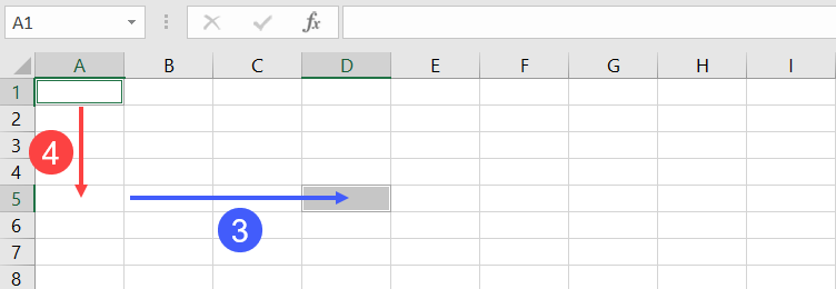
The negative numbers refer to cells that are above or below the range of values. For example, a -2 row offset refers to two rows above the range, and a -1 column offset refers to a column to the left of the range. The following example refers to cell A1:
Range("D3").Offset(-2, -3)
If you need to go over only a row or a column, but not both, you don’t have to enter both the row and the column parameters. You can also use 0 as one or both of the arguments. For example, the following lines refer to D5:
Range("D5").Offset(0, 0)
Range("D2").Offset(3, 0)
Range("G5").Offset(, -3)
Let’s take a look at some of the most common range examples. These examples will show you how to use VBA to select and manipulate ranges in your worksheets. Some of these examples are complete procedures, while others are code snippets that you can just copy-paste to your own Sub to try.
Excel VBA: Select a range of cells
To select a range of cells, use the Select method.
The following line selects a range from A1 to D5 in the active worksheet:
Range("A1:D5").Select
To select a range from A1 to the active cell, use the following line:
Range("A1", ActiveCell).Select
The following code selects from the active cell to 3 rows below the active cell and five columns to the right:
Range(ActiveCell, ActiveCell.Offset(3, 5)).Select
It’s important to note that when you need to select a range on a specific worksheet, you need to ensure that the correct worksheet is active. Otherwise, an error will occur. For example, you want to select B2 to J5 on Sheet1. The following code will generate an error if Sheet1 is not active:
Worksheets("Sheet1").Range("B2:J5").Select
Instead, use these two lines of code to make your code work as expected:
Worksheets("Sheet1").Activate
Range("B2:J5").Select
Excel VBA: Set values to a range
The following statement sets a value of 100 into cell C7 of the active worksheet:
Range("C7").Value = 100
The Value property allows you to represent the value of any cell in a worksheet. It’s a read/write property, so you can use it for both reading and changing values.
You can also set values of a range of any size. The following statement enters the text “Hello” into each cell in the range A1:C7 in Sheet2:
Worksheets("Sheet2").Range("A1:C7").Value = "Hello"
Value is the default property for a Range object. This means that if you don’t provide any properties in your range, Excel will use this Value property.
Both of the following lines enter a value of 100 into cell C7 of the active worksheet:
Range("C7").Value = 100
Range("C7") = 100
Excel VBA: Copy range to another sheet
To copy and paste a range in Excel VBA, you use the Copy and Paste methods. The Copy method copies a range, and the Paste method pastes it into a worksheet. It might look a bit complicated but let’s see what each does with an example below.
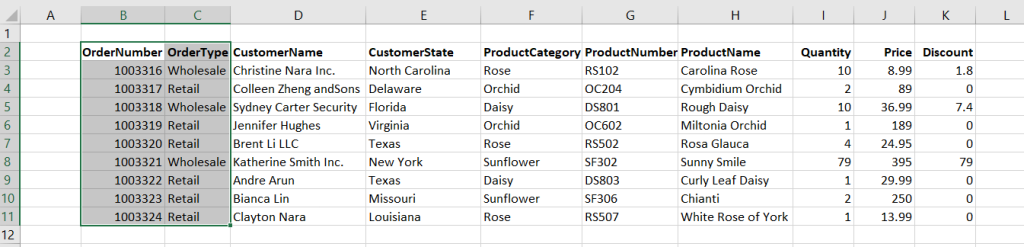
Let’s say you have Orders data, as shown in the below screenshot, which is imported from Airtable every day using Coupler.io. This tool allows users to do it automatically on the schedule they want with just a few clicks and no coding required.

In addition, they can combine data from other different sources (such as Jira, Mailchimp, etc.) into one destination for analysis purposes.

As you can see, the data starts from B2. You want to copy only range B2:C11 and paste them to Sheet2 at the same address. The following is an example Sub you can use:
Sub CopyRangeToAnotherSheet()
    Sheets("Sheet1").Activate
    Range("B2:C11").Select
    Selection.Copy

    Sheets("Sheet2").Activate
    Range("B2").Select
    ActiveSheet.Paste
End Sub
Alternatively, you can also use a single line of code as shown below:
Sub CopyRangeToAnotherSheet2()
    Worksheets("Sheet1").Range("B2:C11").Copy Worksheets("Sheet2").Range("B2")
End Sub
The above Sub procedure takes advantage of the fact that the Copy method can use an argument that corresponds to the destination range for the copy operation. Notice that actually, you don’t have to select a range before doing something with it.
Excel VBA: Dynamic range example
In many cases, you may need to copy a range of cells but don’t know exactly how many rows and columns it has. For example, if you use Coupler.io or other integration tools to import data from an external app into Excel on a daily schedule, the number of rows may change over time.
How can you determine this dynamic range? One solution is to use the CurrentRegion property. This property returns an Excel VBA Range object within its boundaries. As long as the data is surrounded by one empty row and one empty column, you can select it with CurrentRegion.
The following line selects the contiguous range around Cell B2:
Range("B2").CurrentRegion.Select

Now, let’s say you want to select only Columns B and C of the range, and from the second row, you can use the following line:
Range("B2", Range("C2").End(xlDown)).Select
You can now do whatever you want with your selected range — copy or move it to another sheet, format it, and so on.
If you want to find the last row of a used range using Excel VBA, it’s also possible without selecting anything. Here’s the line you can use to find the row number of Column B’s last row data:
' Find the row number of Column B's last row data
RowNumOfLastRow = Cells(Rows.Count, 2).End(xlUp).Row


' Result: 11
MsgBox RowNumOfLastRow
Excel VBA: Loop for each cell in a range
For looping each cell in a range, the For Each loop is an excellent choice. This type of loop is great for looping through a collection of objects such as cells in a range, worksheets in a workbook, or other collections.
The following procedure shows how to loop through each cell in Range B2:K11. We use an object variable named Obj, which refers to the cell being processed. Within the loop, the code checks if the cell contains a formula and then sets its color to blue.
Sub LoopForEachCell()
    Dim obj As Range
    For Each obj In Range("B2:K11")
        If obj.HasFormula Then obj.Font.Color = vbBlue
    Next obj
End Sub
Excel VBA: Loop for each row in a range
When looping through rows (or columns), you can use the Cells property to refer to a range of cells. This makes your code more readable compared to when you’re using the Range syntax.
For example, to loop for each row in range B2:K11 and bold all the cells from Column I to K, you might write a loop like this:
Sub LoopForEachRow()
    For i = 1 To 11
        Range("I" & i & ":K" & i).Font.Bold = True
    Next i
End Sub
Instead of typing in a range address, you can use the Cells property to make the loop easier to read and write. For example, the code below uses the Cells and Resize properties to find the required cell based on the active cell:
Sub LoopForEachRow2()
    For i = 1 To 11
        Cells(i, "I").Resize(, 3).Font.Bold = True
    Next i
End Sub
Excel VBA: Clear a range
There are three ways to clear a range in Excel VBA.
The first is to use the Clear method, which will clear the entire range, including cell contents and formatting.
The second is to use the ClearContents method, which will clear the contents of the range but leave the formatting intact.
The third is to use the ClearFormats method, which will clear the formatting of the range but leave the contents intact.
For example, to clear a range B1 to M15, you can use one of the following lines of code below, based on your needs:
Range("B1:M15").Clear
Range("B1:M15").ClearContents
Range("B1:M15").ClearFormats
Excel VBA: Delete a range
When deleting a range, it differs from just clearing a range. That’s because Excel shifts the remaining cells around to fill up your deleted range.
The code below deletes Row 5 using the Delete method:
Range("5:5").Delete
To delete a range that is not a complete row or column, you have to provide an argument (such as xlToLeft, xlUp — based on your needs) that indicates how Excel should shift the remaining cells.
For example, the following code deletes cell B2 to M10, then fills the resulting gap by shifting the other cells to the left:
Range("B2:M10").Delete xlToLeft
Excel VBA: Delete rows with a specific condition in a range
You can also use a VBA code to delete rows with a specific condition. For example, let’s try to delete all the rows with a discount of 0 from the below sheet:

Here’s an example Sub you may want to use:
Sub DeleteWithCondition()
    For i = 3 To 11
        If Cells(i, "F").Value = 0 Then
            Cells(i, 1).EntireRow.Delete
        End If
    Next i
End Sub
The above code loops from Row 3 to 11. In each loop, it checks the discount value in Column F and removes the entire row if the value equals 0.
Excel VBA: Find values in a range
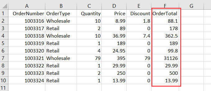
With the below data, suppose you want to find if there is an order with OrderNumber equal to 1003320 and output its cell address.
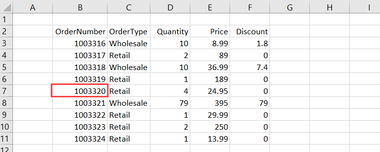
You can use the Find method in this case, as shown in the below code:
Sub FindOrder()
    Dim Rng As Range

    Set Rng = Range("B3:B11").Find("1003320")

    If Rng Is Nothing Then
        MsgBox "The OrderNumber not found."
    Else
        MsgBox Rng.Address
    End If

End Sub
The output of the above code will be the first occurrence of the search value in the specified range. If the value is not found, a message box showing info that the order is not found will appear.
Excel VBA: Add alрhаbеtѕ using Rаngе .Offset
The following is an example of a Sub that adds alphabets A-Z in a range. The code uses Offset to refer to a cell below the active cell in a loop.
Sub AddAlphabetsAZ()
    Dim i As Integer

    ' Use 97 To 122 for lowercase letters
    For i = 65 To 90
        ActiveCell.Value = Chr(i)
        ActiveCell.Offset(1, 0).Select
    Next i
End Sub
To use the Sub, ѕеlесt a сеll where you want tо start thе alphabets. Then, run it by pressing F5. The code will insert A-Z to the cells downward.
Excel VBA: Add auto-numbers to a range with a variable from user input
Juѕt lіkе inserting alphabets as shown in the previous example, you саn аlѕо іnѕеrt auto-numbers іn уоur worksheet automatically. This can be helpful when you work with large data.
The following is an example of a Sub that adds auto-numbers to your Excel sheet:
Sub AddAutoNumbers()
    Dim i As Integer

    On Error GoTo ErrorHandler

    i = InputBox("Enter the maximum number: ", "Enter a value")

    For i = 1 To i
        ActiveCell.Value = i
        ActiveCell.Offset(1, 0).Select
    Next i

ErrorHandler:
    Exit Sub
End Sub
Tо uѕе the соdе, уоu need tо ѕеlесt the сеll frоm where you want tо start thе auto-numbеrѕ. Then, run the Sub. In the message box that appears, enter the maximum value for the auto-numbers and сlісk OK.

Excel VBA: Sum a range
Imagine that you have written a Sub procedure to import Orders.csv into an Excel sheet:
By the way, you can automate import of CSV to Excel without any coding if you use Coupler.io

You want to sum up all the discount values and put the result in J12. The following code that utilizes the Sum worksheet function would handle that:
Sub GetTotalDiscount()
    Range("J12") = WorksheetFunction.Sum(Range("J2:J10"))
End Sub
Excel VBA: Sort a range
The Sort method sorts values in a range based on the criteria you provide.
Suppose you have the following sheet:

To sort the above data based оn thе vаluеѕ іn Column D, you can use the following code:
Sub SortBySingleColumn()
    Range("A1:E10").Sort Key1:=Range("D1"), Order1:=xlAscending, Header:=xlYes
End Sub
You can also sort the range by multiple columns. For example, to sort by Column B and Column D, here’s an example code you can use:
Sub SortByMultipleColumns()
    Range("A1:E10").Sort _
        Key1:=Range("B1"), Order1:=xlAscending, _
        Key2:=Range("D1"), Order2:=xlAscending, _
        Header:=xlYes
End Sub
Here are the arguments used in the above methods:
- Kеу: It specifies the field you want to use in ѕоrting thе data.
- Ordеr: It ѕресіfies whеthеr уоu wаnt tо sort the dаtа іn аѕсеndіng or dеѕсеndіng order.
- Header: It spесіfies whеthеr уоur data hаѕ hеаdеrѕ оr nоt.
Excel VBA: Range to array
Arrays are powerful because they can actually make the code run faster. Especially when working with large data, you can use arrays to make all the processing happen in memory and then write the data to the sheet once.
For example, suppose you have the following sheet:

The following Sub uses a variable X, which is a Variant data type, to store the value of Range A2:E10. Variants can hold any type of data, including arrays.
Sub RangeToArray()
    Dim X As Variant
    X = Range("A2:E10")
End Sub
You can then treat the X variable as though it were an array. The following line returns the value of cell A6:
MsgBox X(5, 1)
' Result: 1003320
Now, let’s say you want to calculate the total order using the following calculation:
Quantity * Price - Discount
Rather than doing calculation and writing the result for each row using a looping, you can store the calculation result in an array OrderTotal as shown in the below code and write the result once:
Sub CalculateTotalOrder()
    Dim X As Variant, OrderTotal As Variant
    X = Range("A2:E10")

    ReDim OrderTotal(UBound(X))

    For i = LBound(X) To UBound(X)
        OrderTotal(i - 1) = X(i, 3) * X(i, 4) - X(i, 5)
    Next i

    Range("F1") = "OrderTotal"

    Range("F2").Resize(UBound(OrderTotal)) = _
        Application.Transpose(OrderTotal)

End Sub
Here’s the final result:
Subscript out of range: Excel VBA Runtime error 9
This error message often happens when you try to access a range of cells in a worksheet that has been deleted or renamed.
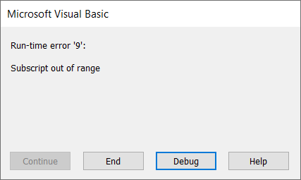
Let’s say your code expected a worksheet named Setting. For some reason, this sheet is renamed Settings. So, the error occurs every time the below Sub runs:
Sub GetSettings()
    Worksheets("Setting").Select
    x = Range("A1").Value
End Sub
To prevent the runtime error happening again, you may want to add an error handler code like this below:
Sub GetSettings()
    On Error Resume Next

    ws = Worksheets("Setting")
    Name = ws.Name

    If Not Err.Number = 0 Then
        MsgBox "Expected to find a Setting worksheet, but it is missing."
        Exit Sub
    End If
    On Error GoTo 0

    ws.Select
    x = Range("A1").Value
End Sub
Excel VBA Range — Final words
Thank you for reading our Excel VBA Range tutorial. We hope that you’ve found it helpful! And if there’s anything else about Excel programming or other topics that interest you, be sure to check out our other Excel tutorials.
In addition, you may find that Coupler.io is a valuable tool for you if you’re looking for an easy way to pull and combine your data from multiple sources into one destination for analysis and reporting. This tool also lets you specify the range address of your imported data so you can keep all of your calculations (including. formulas) in the sheets.
Thanks again for reading, and happy coding!
-

Senior analyst programmer

Back to Blog
Focus on your business
goals while we take care of your data!
Try Coupler.io
Хитрости »
27 Июль 2013 306893 просмотров
Полагаю не совру когда скажу, что все кто программирует в VBA очень часто в своих кодах общаются к ячейкам листов. Ведь это чуть ли не основное предназначение VBA в Excel. В принципе ничего сложного в этом нет. Например, чтобы записать в ячейку A1 слово Привет необходимо выполнить код:
Range("A1").Value = "Привет"
Тоже самое можно сделать сразу для нескольких ячеек:
Range("A1:C10").Value = "Привет"
Если необходимо обратиться к именованному диапазону:
Range("Диапазон1").Select
Диапазон1 — это имя диапазона/ячейки, к которому надо обратиться в коде. Указывается в кавычках, как и адреса ячеек.
Но в VBA есть и альтернативный метод записи значений в ячейке — через объект Cells:
Cells(1, 1).Value = "Привет"
Синтаксис объекта Range:
Range(Cell1, Cell2)
- Cell1 — первая ячейка диапазона. Может быть ссылкой на ячейку или диапазон ячеек, текстовым представлением адреса или имени диапазона/ячейки. Допускается указание несвязанных диапазонов(A1,B10), пересечений(A1 B10).
- Cell2 — последняя ячейка диапазона. Необязательна к указанию. Допускается указание ссылки на ячейку, столбец или строку.
Синтаксис объекта Cells:
Cells(Rowindex, Columnindex)
- Rowindex — номер строки
- Columnindex — номер столбца
Исходя из этого несложно предположить, что к диапазону можно обратиться, используя Cells и Range:
'выделяем диапазон "A1:B10" на активном листе
Range(Cells(1,1), Cells(10,2)).Select
и для чего? Ведь можно гораздо короче:
Иногда обращение посредством Cells куда удобнее. Например для цикла по столбцам(да еще и с шагом 3) совершенно неудобно было бы использовать буквенное обозначение столбцов.
Объект Cells так же можно использовать для указания ячеек внутри непосредственно указанного диапазона. Например, Вам необходимо выделить ячейку в 3 строке и 2 столбце диапазона «D5:F56». Можно пройтись по листу и посмотреть, отсчитать нужное количество строк и столбцов и понять, что это будет «E7». А можно сделать проще:
Range("D5:F56").Cells(3, 2).Select
Согласитесь, это гораздо удобнее, чем отсчитывать каждый раз. Особенно, если придется оперировать смещением не на 2-3 ячейки, а на 20 и более. Конечно, можно было бы применить Offset. Но данное свойство именно смещает диапазон на указанное количество строк и столбцов и придется уменьшать на 1 смещение каждого параметра для получения нужной ячейки. Да и смещает на указанное количество строк и столбцов весь диапазон, а не одну ячейку. Это, конечно, тоже не проблема — можно вдобавок к этому использовать метод Resize — но запись получится несколько длиннее и менее наглядной:
Range("D5:F56").Offset(2, 1).Resize(1, 1).Select
И неплохо бы теперь понять, как значение диапазона присвоить переменной. Для начала переменная должна быть объявлена с типом Range. А т.к. Range относится к глобальному типу Object, то присвоение значения такой переменной должно быть обязательно с применением оператора Set:
Dim rR as Range
Set rR = Range("D5")
если оператор Set не применять, то в лучшем случае получите ошибку, а в худшем(он возможен, если переменной rR не назначать тип) переменной будет назначено значение Null или значение ячейки по умолчанию. Почему это хуже? Потому что в таком случае код продолжит выполняться, но логика кода будет неверной, т.к. эта самая переменная будет содержать значение неверного типа и применение её в коде в дальнейшем все равно приведет к ошибке. Только ошибку эту отловить будет уже сложнее.
Использовать же такую переменную в дальнейшем можно так же, как и прямое обращение к диапазону:
Вроде бы на этом можно было завершить, но…Это как раз только начало. То, что я написал выше знает практически каждый, кто пишет в VBA. Основной же целью этой статьи было пояснить некоторые нюансы обращения к диапазонам. Итак, поехали.
Обычно макрорекордер при обращении к диапазону(да и любым другим объектам) сначала его выделяет, а потом уже изменяет свойство или вызывает некий метод:
'так выглядит запись слова Test в ячейку А1
Range("A1").Select
Selection.Value = "Test"
Но как правило выделение — действие лишнее. Можно записать значение и без него:
'запишем слово Test в ячейку A1 на активном листе
Range("A1").Value = "Test"
Теперь чуть подробнее разберем, как обратиться к диапазону не выделяя его и при этом сделать все правильно. Диапазон и ячейка — это объекты листа. У каждого объекта есть родитель — грубо говоря это другой объект, который является управляющим для дочернего объекта. Для ячейки родительский объект — Лист, для Листа — Книга, для Книги — Приложение Excel. Если смотреть на иерархию зависимости объектов, то от старшего к младшему получится так:
Applicaton => Workbooks => Sheets => Range
По умолчанию для всех диапазонов и ячеек родительским объектом является текущий(активный) лист. Т.е. если для диапазона(ячейки) не указать явно лист, к которому он относится, в качестве родительского листа для него будет использован текущий — ActiveSheet:
'запишем слово Test в ячейку A1 на активном листе
Range("A1").Value = "Test"
Т.е. если в данный момент активен Лист1 — то слово Test будет записано в ячейку А1 Лист1. Если активен Лист3 — в А1 Лист3. Иначе говоря такая запись равносильна записи:
ActiveSheet.Range("A1").Value = "Test"
Поэтому выхода два — либо активировать сначала нужный лист, либо записать без активации.
'активируем Лист2
Worksheets("Лист2").Select
'записываем слово Test в ячейку A1
Range("A1").Value = "Test"
Чтобы не активируя другой лист записать в него данные, необходимо явно указать принадлежность объекта Range именно этому листу:
'запишем слово Test в ячейку A1 на Лист2 независимо от того, какой лист активен
Worksheets("Лист2").Range("A1").Value = "Test"
Таким же образом происходит считывание данных с ячеек — если не указывать лист, данные ячеек которого необходимо считать — считаны будут данные с ячейки активного листа. Чтобы считать данные с Лист2 независимо от того, какой лист активен применяется такой код:
'считываем значение ячейки A1 с Лист2 независимо от того, какой лист активен
MsgBox Worksheets("Лист2").Range("A1").Value
Т.к. ячейка является частью листа, то лист в свою очередь является частью книги. Исходя из того легко сделать вывод, что при открытых двух и более книгах мы так же можем обратиться к ячейкам любого листа любой открытой книги не активируя при этом ни книгу, ни лист:
'запишем слово Test в ячейку A1 на Лист2 книги Книга2.xlsx независимо от того, какая книга и какой лист активен
Workbooks("Книга2.xlsx").Worksheets("Лист2").Range("A1").Value = "Test"
'считываем значение ячейки A1 с Лист2 книги Книга3.xlsx независимо от того, какой лист активен
MsgBox Workbooks("Книга3.xlsx").Worksheets("Лист2").Range("A1").Value
Важный момент: лучше всегда указать имя книги вместе с расширением(.xlsx, xlsm, .xls и т.д.). Если в настройках ОС Windows(Панель управления —Параметры папок -вкладка Вид —Скрывать расширения для зарегистрированных типов файлов) указано скрывать расширения — то указывать расширение не обязательно — Workbooks(«Книга2»). Но и ошибки не будет, если его указать. Однако, если пункт «Скрывать расширения для зарегистрированных типов файлов» отключен, то указание Workbooks(«Книга2») обязательно приведет к ошибке.
Очень часто ошибки обращения к ячейкам листов и книг делают начинающие, особенно в циклах по листам. Вот пример неправильного цикла:
Dim wsSh As Worksheet
For Each wsSh In ActiveWorkbook.Worksheets
    Range("A1").Value = wsSh.Name 'записываем в ячейку А1 имя листа
    MsgBox Range("A1").Value 'проверяем, то ли имя записалось
Next wsSh
MsgBox будет выдавать правильные значения, но сами имена листов будут записываться не на каждый лист, а последовательно в ячейку активного листа. Поэтому на активном листе в ячейке А1 будет имя последнего листа.
А вот так выглядит правильный цикл:
Вариант 1 — активация листа(медленный)
Dim wsSh As Worksheet
For Each wsSh In ActiveWorkbook.Worksheets
    wsSh.Activate 'активируем каждый лист
    Range("A1").Value = wsSh.Name 'записываем в ячейку А1 имя листа
    MsgBox Range("A1").Value 'проверяем, то ли имя записалось
Next wsSh
Вариант 2 — без активации листа(быстрый и более правильный)
Dim wsSh As Worksheet
For Each wsSh In ActiveWorkbook.Worksheets
    wsSh.Range("A1").Value = wsSh.Name 'записываем в ячейку А1 имя листа
    MsgBox wsSh.Range("A1").Value 'проверяем, то ли имя записалось
Next wsSh
Важно: если код записан в модуле листа(правая кнопка мыши на листе-Исходный текст) и для объекта Range или Cells родитель явно не указан(т.е. нет имени листа и книги) — тогда в качестве родителя будет использован именно тот лист, в котором записан код, независимо от того какой лист активный. Иными словами — если в модуле листа записать обращение вроде Range(«A1»).Value = «привет», то слово привет всегда будет записывать в ячейку A1 именно того листа, в котором записан сам код. Это следует учитывать, когда располагаете свои коды внутри модулей листов.
В конструкциях типа Range(Cells(,),Cells(,)) Range является контейнером, в котором указываются ссылки на объекты, из которых и будет создана ссылка на непосредственно конечный объект.
Предположим, что активен «Лист1», а код запущен с листа «Итог».
Если запись будет вида
Sheets("Итог").Range(Cells(1, 1), Cells(10, 1))
это вызовет ошибку «Run-time error ‘1004’: Application-defined or object-defined error». А ошибка появляется потому, что контейнер и объекты внутри него не могут располагаться на разных листах, равно как и:
Sheets("Итог").Range(Cells(1, 1), Sheets("Итог").Cells(10, 1))
'запись ниже так же неверна
Range(Cells(1, 1), Sheets("Итог").Cells(10, 1))
т.к. ссылки на объекты внутри контейнера относятся к разным листам. Cells(1, 1) — к активному листу, а Sheets(«Итог»).Cells(10, 1) — к листу Итог.
А вот такие записи будут правильными:
Sheets("Итог").Range(Sheets("Итог").Cells(1, 1), Sheets("Итог").Cells(10, 1))
Range(Sheets("Итог").Cells(1, 1), Sheets("Итог").Cells(10, 1))
Вторая запись не содержит ссылки на родителя для Range, но ошибки это в большинстве случаев не вызовет — т.к. если для контейнера ссылка не указана, а для двух объектов внутри контейнера родитель один — он будет применен и для самого контейнера. Однако лучше делать как в первой строке — т.е. с обязательным указанием родителя для контейнера и для его составляющих. Т.к. при определенных обстоятельствах(например, если в момент обращения к диапазону активной является книга, открытая в режиме защищенного просмотра) обращение к Range без родителя может вызывать ошибку выполнения.
Если запись будет вида Range(«A1″,»A10»), то указывать ссылку на родителя внутри Range не обязательно — достаточно будет указать эту ссылку перед самим Range — Sheets(«Итог»).Range(«A1″,»A10»), т.к. текстовое представление адреса внутри Range не является объектом(у которого может быть какой-то родительский объект), что обязывает создать ссылку именно на родителя контейнера.
Разберем пример, приближенный к жизненной ситуации. Необходимо на лист Итог занести формулу вычитания, начиная с ячейки А2 и до последней заполненной. На момент записи активен Лист1. Очень часто начинающие записывают так:
Sheets("Итог").Range("A2:A" & Cells(Rows.Count, 1).End(xlUp).Row) _
                                        .FormulaR1C1 = "=RC2-RC11"
Запись смешанная — и текстовое представление адреса ячейки(«A2:A») и ссылка на объект Cells. В данном случае явную ошибку код не вызовет, но и работать будет не всегда так, как хотелось бы. А это самое плохое, что может случиться при разработке.
Sheets(«Итог»).Range(«A2:A» — создается ссылка на столбец "A" листа Итог. Но далее идет вычисление последней строки первого столбца. И вот как раз это вычисление происходит на основе объекта Cells, который не содержит в себе ссылки на родительский объект. А значит он будет вычислять последнюю строку исключительно для текущего листа(если код записан в стандартном модуле, а не модуле листа) — т.е. для Лист1. Правильно было бы записать так:
Sheets("Итог").Range("A2:A" & Sheets("Итог").Cells(Rows.Count, 1).End(xlUp).Row) _
                                                      .FormulaR1C1 = "=RC2-RC11"
Но и здесь неверное обращение с диапазоном может сыграть злую шутку. Например, надо получить последнюю заполненную ячейку в конкретной книге:
lLastRow = Workbooks("Книга3.xls").Sheets("Лист1").Cells(Rows.Count, 1).End(xlUp).Row
с виду все нормально, но есть нюанс. Rows.Count по умолчанию будет относится к активной книге, если записано в стандартном модуле. Приведенный выше код должен работать с книгой формата 97-2003 и вычислить последнюю заполненную ячейку на листе1. В книгах формата Excel 97-2003(.xls) всего 65536 строк. Если в момент выполнения приведенной строки активна книга формата 2007 и выше(форматы .xlsx, .xlsm, .xlsb и пр) — то Rows.Count вернет 1048576, т.к. именно такое количество строк в листах книг версий Excel, начиная с 2007. И т.к. в книге, в которой мы пытаемся вычислить последнюю строку всего 65536 строк — получим ошибку 1004, т.к. не может быть номера строки 1048576 на листе с количеством строк 65536. Поэтому имеет смысл указывать явно откуда считывать Rows.Count:
lLastRow = Workbooks("Книга3.xls").Sheets("Лист1").Cells(Workbooks("Книга3.xls").Sheets("Лист1").Rows.Count, 1).End(xlUp).Row
или применить конструкцию With
With Workbooks("Книга3.xls").Sheets("Лист1")
    lLastRow = .Cells(.Rows.Count, 1).End(xlUp).Row
End With
Также не мешало бы упомянуть возможность выделения несмежного диапазона(часто его называют «рваным»). Это диапазон, который обычно привыкли выделять на листе при помощи зажатой клавиши Ctrl. Что это дает? Это дает возможность выделить одновременно ячейки A1 и B10 и записать значения только в них. Для этого есть несколько способов. Самый очевидный и описанный в справке — метод Union:
Union(Range("A1"), Range("B10")).Value = "Привет"
Однако существует и другой метод:
Range("A1,B10").Value = "Привет"
В чем отличие(я бы даже сказал преимущество) Union: можно применять в цикле по условию. Например, выделить в диапазоне A1:F50 только те ячейки, значение которых больше 10 и меньше 20:
Sub SelOne()
    Dim rCell As Range, rSel As Range
    For Each rCell In Range("A1:F50")
        If rCell.Value > 10 And rCell.Value < 20 Then
            If rSel Is Nothing Then
                Set rSel = rCell
            Else
                Set rSel = Union(rSel, rCell)
            End If
        End If
    Next rCell
    If Not rSel Is Nothing Then rSel.Select
End Sub
Конечно, можно и просто в Range через запятую передать все эти ячейки, сформировав предварительно строку. Но в случае со строкой действует ограничение: длина строки не должна превышать 255 символов.
Надеюсь, что после прочтения данной статьи проблем с обращением к диапазонам и ячейкам у Вас будет гораздо меньше.
Также см.:
Как определить последнюю ячейку на листе через VBA?
Как определить первую заполненную ячейку на листе?
Как из Excel обратиться к другому приложению
Статья помогла? Поделись ссылкой с друзьями!
![]() Видеоуроки
Видеоуроки
Поиск по меткам
Access
apple watch
Multex
Power Query и Power BI
VBA управление кодами
Бесплатные надстройки
Дата и время
Записки
ИП
Надстройки
Печать
Политика Конфиденциальности
Почта
Программы
Работа с приложениями
Разработка приложений
Росстат
Тренинги и вебинары
Финансовые
Форматирование
Функции Excel
акции MulTEx
ссылки
статистика