
Всё о работе с ячейками в Excel-VBA: обращение, перебор, удаление, вставка, скрытие, смена имени.
Содержание:
Table of Contents:
- Что такое ячейка Excel?
- Способы обращения к ячейкам
- Выбор и активация
- Получение и изменение значений ячеек
- Ячейки открытой книги
- Ячейки закрытой книги
- Перебор ячеек
- Перебор в произвольном диапазоне
- Свойства и методы ячеек
- Имя ячейки
- Адрес ячейки
- Размеры ячейки
- Запуск макроса активацией ячейки
2 нюанса:
- Я почти везде стараюсь использовать ThisWorkbook (а не, например, ActiveWorkbook) для обращения к текущей книге, в которой написан этот код (считаю это наиболее безопасным для новичков способом обращения к книгам, чтобы случайно не внести изменения в другие книги). Для экспериментов можете вставлять этот код в модули, коды книги, либо листа, и он будет работать только в пределах этой книги.
- Я использую английский эксель и у меня по стандарту листы называются Sheet1, Sheet2 и т.д. Если вы работаете в русском экселе, то замените Thisworkbook.Sheets(«Sheet1») на Thisworkbook.Sheets(«Лист1»). Если этого не сделать, то вы получите ошибку в связи с тем, что пытаетесь обратиться к несуществующему объекту. Можно также заменить на Thisworkbook.Sheets(1), но это менее безопасно.
Что такое ячейка Excel?
В большинстве мест пишут: «элемент, образованный пересечением столбца и строки». Это определение полезно для людей, которые не знакомы с понятием «таблица». Для того, чтобы понять чем на самом деле является ячейка Excel, необходимо заглянуть в объектную модель Excel. При этом определения объектов «ряд», «столбец» и «ячейка» будут отличаться в зависимости от того, как мы работаем с файлом.
Объекты в Excel-VBA. Пока мы работаем в Excel без углубления в VBA определение ячейки как «пересечения» строк и столбцов нам вполне хватает, но если мы решаем как-то автоматизировать процесс в VBA, то о нём лучше забыть и просто воспринимать лист как «мешок» ячеек, с каждой из которых VBA позволяет работать как минимум тремя способами:
- по цифровым координатам (ряд, столбец),
- по адресам формата А1, B2 и т.д. (сценарий целесообразности данного способа обращения в VBA мне сложно представить)
- по уникальному имени (во втором и третьем вариантах мы будем иметь дело не совсем с ячейкой, а с объектом VBA range, который может состоять из одной или нескольких ячеек). Функции и методы объектов Cells и Range отличаются. Новичкам я бы порекомендовал работать с ячейками VBA только с помощью Cells и по их цифровым координатам и использовать Range только по необходимости.
Все три способа обращения описаны далее
Как это хранится на диске и как с этим работать вне Excel? С точки зрения хранения и обработки вне Excel и VBA. Сделать это можно, например, сменив расширение файла с .xls(x) на .zip и открыв этот архив.
Пример содержимого файла Excel:
Далее xl -> worksheets и мы видим файл листа
Содержимое файла:
То же, но более наглядно:
<?xml version="1.0" encoding="UTF-8" standalone="yes"?>
<worksheet xmlns="http://schemas.openxmlformats.org/spreadsheetml/2006/main" xmlns:r="http://schemas.openxmlformats.org/officeDocument/2006/relationships" xmlns:mc="http://schemas.openxmlformats.org/markup-compatibility/2006" mc:Ignorable="x14ac xr xr2 xr3" xmlns:x14ac="http://schemas.microsoft.com/office/spreadsheetml/2009/9/ac" xmlns:xr="http://schemas.microsoft.com/office/spreadsheetml/2014/revision" xmlns:xr2="http://schemas.microsoft.com/office/spreadsheetml/2015/revision2" xmlns:xr3="http://schemas.microsoft.com/office/spreadsheetml/2016/revision3" xr:uid="{00000000-0001-0000-0000-000000000000}">
	<dimension ref="B2:F6"/>
	<sheetViews>
		<sheetView tabSelected="1" workbookViewId="0">
			<selection activeCell="D12" sqref="D12"/>
		</sheetView>
	</sheetViews>
	<sheetFormatPr defaultRowHeight="14.4" x14ac:dyDescent="0.3"/>
	<sheetData>
		<row r="2" spans="2:6" x14ac:dyDescent="0.3">
			<c r="B2" t="s">
				<v>0</v>
			</c>
		</row>
		<row r="3" spans="2:6" x14ac:dyDescent="0.3">
			<c r="C3" t="s">
				<v>1</v>
			</c>
		</row>
		<row r="4" spans="2:6" x14ac:dyDescent="0.3">
			<c r="D4" t="s">
				<v>2</v>
			</c>
		</row>
		<row r="5" spans="2:6" x14ac:dyDescent="0.3">
			<c r="E5" t="s">
				<v>0</v></c>
		</row>
		<row r="6" spans="2:6" x14ac:dyDescent="0.3">
			<c r="F6" t="s"><v>3</v>
		</c></row>
	</sheetData>
	<pageMargins left="0.7" right="0.7" top="0.75" bottom="0.75" header="0.3" footer="0.3"/>
</worksheet>
Как мы видим, в структуре объектной модели нет никаких «пересечений». Строго говоря рабочая книга — это архив структурированных данных в формате XML. При этом в каждую «строку» входит «столбец», и в нём в свою очередь прописан номер значения данного столбца, по которому оно подтягивается из другого XML файла при открытии книги для экономии места за счёт отсутствия повторяющихся значений. Почему это важно. Если мы захотим написать какой-то обработчик таких файлов, который будет напрямую редактировать данные в этих XML, то ориентироваться надо на такую модель и структуру данных. И правильное определение будет примерно таким: ячейка — это объект внутри столбца, который в свою очередь находится внутри строки в файле xml, в котором хранятся данные о содержимом листа.
Способы обращения к ячейкам
Выбор и активация
Почти во всех случаях можно и стоит избегать использования методов Select и Activate. На это есть две причины:
- Это лишь имитация действий пользователя, которая замедляет выполнение программы. Работать с объектами книги можно напрямую без использования методов Select и Activate.
- Это усложняет код и может приводить к неожиданным последствиям. Каждый раз перед использованием Select необходимо помнить, какие ещё объекты были выбраны до этого и не забывать при необходимости снимать выбор. Либо, например, в случае использования метода Select в самом начале программы может быть выбрано два листа вместо одного потому что пользователь запустил программу, выбрав другой лист.
Можно выбирать и активировать книги, листы, ячейки, фигуры, диаграммы, срезы, таблицы и т.д.
Отменить выбор ячеек можно методом Unselect:
Selection.UnselectОтличие выбора от активации — активировать можно только один объект из раннее выбранных. Выбрать можно несколько объектов.
Если вы записали и редактируете код макроса, то лучше всего заменить Select и Activate на конструкцию With … End With. Например, предположим, что мы записали вот такой макрос:
Sub Macro1()
' Macro1 Macro
    Range("F4:F10,H6:H10").Select 'выбрали два несмежных диапазона зажав ctrl
    Range("H6").Activate          'показывает только то, что я начал выбирать второй диапазон с этой ячейки (она осталась белой). Это действие ни на что не влияет
    With Selection.Interior
        .Pattern = xlSolid
        .PatternColorIndex = xlAutomatic
        .Color = 65535            'залили желтым цветом, нажав на кнопку заливки на верхней панели
        .TintAndShade = 0
        .PatternTintAndShade = 0
    End With
End Sub
Почему макрос записался таким неэффективным образом? Потому что в каждый момент времени (в каждой строке) программа не знает, что вы будете делать дальше. Поэтому в записи выбор ячеек и действия с ними — это два отдельных действия. Этот код лучше всего оптимизировать (особенно если вы хотите скопировать его внутрь какого-нибудь цикла, который должен будет исполняться много раз и перебирать много объектов). Например, так:
Sub Macro11()
'
' Macro1 Macro
    Range("F4:F10,H6:H10").Select '1. смотрим, что за объект выбран (что идёт до .Select)
    Range("H6").Activate
    With Selection.Interior       '2. понимаем, что у выбранного объекта есть свойство interior, с которым далее идёт работа
        .Pattern = xlSolid
        .PatternColorIndex = xlAutomatic
        .Color = 65535
        .TintAndShade = 0
        .PatternTintAndShade = 0
    End With
End Sub


Sub Optimized_Macro()
    With Range("F4:F10,H6:H10").Interior '3. переносим объект напрямую в конструкцию With вместо Selection
' ////// Здесь я для надёжности прописал бы ещё Thisworkbook.Sheet("ИмяЛиста") перед Range,
' ////// чтобы минимизировать риск любых случайных изменений других листов и книг
' ////// With Thisworkbook.Sheet("ИмяЛиста").Range("F4:F10,H6:H10").Interior
        .Pattern = xlSolid               '4. полностью копируем всё, что было записано рекордером внутрь блока with
        .PatternColorIndex = xlAutomatic
        .Color = 55555                   '5. здесь я поменял цвет на зеленый, чтобы было видно, работает ли код при поочерёдном запуске двух макросов
        .TintAndShade = 0
        .PatternTintAndShade = 0
    End With
End Sub
Пример сценария, когда использование Select и Activate оправдано:
Допустим, мы хотим, чтобы во время исполнения программы мы одновременно изменяли несколько листов одним действием и пользователь видел какой-то определённый лист. Это можно сделать примерно так:
Sub Select_Activate_is_OK()
Thisworkbook.Worksheets(Array("Sheet1", "Sheet3")).Select 'Выбираем несколько листов по именам
Thisworkbook.Worksheets("Sheet3").Activate 'Показываем пользователю третий лист
'Далее все действия с выбранными ячейками через Select будут одновременно вносить изменения в оба выбранных листа

'Допустим, что тут мы решили покрасить те же два диапазона:
Range("F4:F10,H6:H10").Select
    Range("H6").Activate
    With Selection.Interior
        .Pattern = xlSolid
        .PatternColorIndex = xlAutomatic
        .Color = 65535
        .TintAndShade = 0
        .PatternTintAndShade = 0
    End With

End Sub
Единственной причиной использовать этот код по моему мнению может быть желание зачем-то показать пользователю определённую страницу книги в какой-то момент исполнения программы. С точки зрения обработки объектов, опять же, эти действия лишние.
Получение и изменение значений ячеек
Значение ячеек можно получать/изменять с помощью свойства value.
'Если нужно прочитать / записать значение ячейки, то используется свойство Value
a = ThisWorkbook.Sheets("Sheet1").Cells (1,1).Value 'записать значение ячейки А1 листа "Sheet1" в переменную "a"
ThisWorkbook.Sheets("Sheet1").Cells (1,1).Value = 1  'задать значение ячейки А1 (первый ряд, первый столбец) листа "Sheet1"

'Если нужно прочитать текст как есть (с форматированием), то можно использовать свойство .text:
ThisWorkbook.Sheets("Sheet1").Cells (1,1).Text = "1"
a = ThisWorkbook.Sheets("Sheet1").Cells (1,1).Text

'Когда проявится разница:
'Например, если мы считываем дату в формате "31 декабря 2021 г.", хранящуюся как дата
a = ThisWorkbook.Sheets("Sheet1").Cells (1,1).Value 'эапишет как "31.12.2021"
a = ThisWorkbook.Sheets("Sheet1").Cells (1,1).Text  'запишет как "31 декабря 2021 г."
Ячейки открытой книги
К ячейкам можно обращаться:
'В книге, в которой хранится макрос (на каком-то из листов, либо в отдельном модуле или форме)
ThisWorkbook.Sheets("Sheet1").Cells(1,1).Value        'По номерам строки и столбца
ThisWorkbook.Sheets("Sheet1").Cells(1,"A").Value      'По номерам строки и букве столбца
ThisWorkbook.Sheets("Sheet1").Range("A1").Value       'По адресу - вариант 1
ThisWorkbook.Sheets("Sheet1").[A1].Value              'По адресу - вариант 2
ThisWorkbook.Sheets("Sheet1").Range("CellName").Value 'По имени ячейки (для этого ей предварительно нужно его присвоить)

'Те же действия, но с использованием полного названия рабочей книги (книга должна быть открыта)
Workbooks("workbook.xlsm").Sheets("Sheet1").Cells(1,1).Value 'По номерам строки и столбца
Workbooks("workbook.xlsm").Sheets("Sheet1").Cells(1,"A").Value                'По номерам строки и букве столбца
Workbooks("workbook.xlsm").Sheets("Sheet1").Range("A1").Value                 'По адресу - вариант 1
Workbooks("workbook.xlsm").Sheets("Sheet1").[A1].Value                        'По адресу - вариант 2
Workbooks("workbook.xlsm").Sheets("Sheet1").Range("CellName").Value           'По имени ячейки (для этого ей предварительно нужно его присвоить)
Ячейки закрытой книги
Если нужно достать или изменить данные в другой закрытой книге, то необходимо прописать открытие и закрытие книги. Непосредственно работать с закрытой книгой не получится, потому что данные в ней хранятся отдельно от структуры и при открытии Excel каждый раз производит расстановку значений по соответствующим «слотам» в структуре. Подробнее о том, как хранятся данные в xlsx см выше.
Workbooks.Open Filename:="С:closed_workbook.xlsx"    'открыть книгу (она становится активной)
a = ActiveWorkbook.Sheets("Sheet1").Cells(1,1).Value  'достать значение ячейки 1,1
ActiveWorkbook.Close False                            'закрыть книгу (False => без сохранения)
Скачать пример, в котором можно посмотреть, как доставать и как записывать значения в закрытую книгу.
Код из файла:
Option Explicit
Sub get_value_from_closed_wb() 'достать значение из закрытой книги
Dim a, wb_path, wsh As String
wb_path = ThisWorkbook.Sheets("Sheet1").Cells(2, 3).Value 'get path to workbook from sheet1
wsh = ThisWorkbook.Sheets("Sheet1").Cells(3, 3).Value
Workbooks.Open Filename:=wb_path
a = ActiveWorkbook.Sheets(wsh).Cells(3, 3).Value
ActiveWorkbook.Close False
ThisWorkbook.Sheets("Sheet1").Cells(4, 3).Value = a
End Sub

Sub record_value_to_closed_wb() 'записать значение в закрытую книгу
Dim wb_path, b, wsh As String
wsh = ThisWorkbook.Sheets("Sheet1").Cells(3, 3).Value
wb_path = ThisWorkbook.Sheets("Sheet1").Cells(2, 3).Value 'get path to workbook from sheet1
b = ThisWorkbook.Sheets("Sheet1").Cells(5, 3).Value 'get value to record in the target workbook
Workbooks.Open Filename:=wb_path
ActiveWorkbook.Sheets(wsh).Cells(4, 4).Value = b 'add new value to cell D4 of the target workbook
ActiveWorkbook.Close True
End Sub
Перебор ячеек
Перебор в произвольном диапазоне
Скачать файл со всеми примерами
Пройтись по всем ячейкам в нужном диапазоне можно разными способами. Основные:
- Цикл For Each. Пример:
Sub iterate_over_cells() For Each c In ThisWorkbook.Sheets("Sheet1").Range("B2:D4").Cells MsgBox (c) Next c End SubЭтот цикл выведет в виде сообщений значения ячеек в диапазоне B2:D4 по порядку по строкам слева направо и по столбцам — сверху вниз. Данный способ можно использовать для действий, в который вам не важны номера ячеек (закрашивание, изменение форматирования, пересчёт чего-то и т.д.).
- Ту же задачу можно решить с помощью двух вложенных циклов — внешний будет перебирать ряды, а вложенный — ячейки в рядах. Этот способ я использую чаще всего, потому что он позволяет получить больше контроля над исполнением: на каждой итерации цикла нам доступны координаты ячеек. Для перебора всех ячеек на листе этим методом потребуется найти последнюю заполненную ячейку. Пример кода:
Sub iterate_over_cells() Dim cl, rw As Integer Dim x As Variant 'перебор области 3x3 For rw = 1 To 3 ' цикл для перебора рядов 1-3 For cl = 1 To 3 'цикл для перебора столбцов 1-3 x = ThisWorkbook.Sheets("Sheet1").Cells(rw + 1, cl + 1).Value MsgBox (x) Next cl Next rw 'перебор всех ячеек на листе. Последняя ячейка определена с помощью UsedRange 'LastRow = ActiveSheet.UsedRange.Row + ActiveSheet.UsedRange.Rows.Count - 1 'LastCol = ActiveSheet.UsedRange.Column + ActiveSheet.UsedRange.Columns.Count - 1 'For rw = 1 To LastRow 'цикл перебора всех рядов ' For cl = 1 To LastCol 'цикл для перебора всех столбцов ' Действия ' Next cl 'Next rw End Sub - Если нужно перебрать все ячейки в выделенном диапазоне на активном листе, то код будет выглядеть так:
Sub iterate_cell_by_cell_over_selection() Dim ActSheet As Worksheet Dim SelRange As Range Dim cell As Range Set ActSheet = ActiveSheet Set SelRange = Selection 'if we want to do it in every cell of the selected range For Each cell In Selection MsgBox (cell.Value) Next cell End SubДанный метод подходит для интерактивных макросов, которые выполняют действия над выбранными пользователем областями.
- Перебор ячеек в ряду
Sub iterate_cells_in_row() Dim i, RowNum, StartCell As Long RowNum = 3 'какой ряд StartCell = 0 ' номер начальной ячейки (минус 1, т.к. в цикле мы прибавляем i) For i = 1 To 10 ' 10 ячеек в выбранном ряду ThisWorkbook.Sheets("Sheet1").Cells(RowNum, i + StartCell).Value = i '(i + StartCell) добавляет 1 к номеру столбца при каждом повторении Next i End Sub - Перебор ячеек в столбце
Sub iterate_cells_in_column() Dim i, ColNum, StartCell As Long ColNum = 3 'какой столбец StartCell = 0 ' номер начальной ячейки (минус 1, т.к. в цикле мы прибавляем i) For i = 1 To 10 ' 10 ячеек ThisWorkbook.Sheets("Sheet1").Cells(i + StartCell, ColNum).Value = i ' (i + StartCell) добавляет 1 к номеру ряда при каждом повторении Next i End Sub
Свойства и методы ячеек
Имя ячейки
Присвоить новое имя можно так:
Thisworkbook.Sheets(1).Cells(1,1).name = "Новое_Имя"Для того, чтобы сменить имя ячейки нужно сначала удалить существующее имя, а затем присвоить новое. Удалить имя можно так:
ActiveWorkbook.Names("Старое_Имя").DeleteПример кода для переименования ячеек:
Sub rename_cell()

old_name = "Cell_Old_Name"
new_name = "Cell_New_Name"

ActiveWorkbook.Names(old_name).Delete
ThisWorkbook.Sheets(1).Cells(2, 1).Name = new_name
End Sub

Sub rename_cell_reverse()

old_name = "Cell_New_Name"
new_name = "Cell_Old_Name"

ActiveWorkbook.Names(old_name).Delete
ThisWorkbook.Sheets(1).Cells(2, 1).Name = new_name
End Sub
Адрес ячейки
Sub get_cell_address() ' вывести адрес ячейки в формате буква столбца, номер ряда
  '$A$1 style
  txt_address = ThisWorkbook.Sheets(1).Cells(3, 2).Address
  MsgBox (txt_address)
End Sub

Sub get_cell_address_R1C1()' получить адрес столбца в формате номер ряда, номер столбца
  'R1C1 style
  txt_address = ThisWorkbook.Sheets(1).Cells(3, 2).Address(ReferenceStyle:=xlR1C1)
  MsgBox (txt_address)
End Sub

  'пример функции, которая принимает 2 аргумента: название именованного диапазона и тип желаемого адреса
  '(1- тип $A$1 2- R1C1 - номер ряда, столбца)
Function get_cell_address_by_name(str As String, address_type As Integer)
  '$A$1 style
  Select Case address_type
    Case 1
      txt_address = Range(str).Address
    Case 2
      txt_address = Range(str).Address(ReferenceStyle:=xlR1C1)
    Case Else
      txt_address = "Wrong address type selected. 1,2 available"
    End Select
  get_cell_address_by_name = txt_address
End Function

'перед запуском нужно убедиться, что в книге есть диапазон с названием,
'адрес которого мы хотим получить, иначе будет ошибка
Sub test_function() 'запустите эту программу, чтобы увидеть, как работает функция
  x = get_cell_address_by_name("MyValue", 2)
  MsgBox (x)
End Sub
Размеры ячейки
Ширина и длина ячейки в VBA меняется, например, так:
Sub change_size()
Dim x, y As Integer
Dim w, h As Double

'получить координаты целевой ячейки
x = ThisWorkbook.Sheets("Sheet1").Cells(2, 2).Value
y = ThisWorkbook.Sheets("Sheet1").Cells(3, 2).Value

'получить желаемую ширину и высоту ячейки
w = ThisWorkbook.Sheets("Sheet1").Cells(6, 2).Value
h = ThisWorkbook.Sheets("Sheet1").Cells(7, 2).Value

'сменить высоту и ширину ячейки с координатами x,y
ThisWorkbook.Sheets("Sheet1").Cells(x, y).RowHeight = h
ThisWorkbook.Sheets("Sheet1").Cells(x, y).ColumnWidth = w


End Sub
Прочитать значения ширины и высоты ячеек можно двумя способами (однако результаты будут в разных единицах измерения). Если написать просто Cells(x,y).Width или Cells(x,y).Height, то будет получен результат в pt (привязка к размеру шрифта).
Sub get_size()
Dim x, y As Integer
'получить координаты ячейки, с которой мы будем работать
x = ThisWorkbook.Sheets("Sheet1").Cells(2, 2).Value
y = ThisWorkbook.Sheets("Sheet1").Cells(3, 2).Value

'получить длину и ширину выбранной ячейки в тех же единицах измерения, в которых мы их задавали
ThisWorkbook.Sheets("Sheet1").Cells(2, 6).Value = ThisWorkbook.Sheets("Sheet1").Cells(x, y).ColumnWidth
ThisWorkbook.Sheets("Sheet1").Cells(3, 6).Value = ThisWorkbook.Sheets("Sheet1").Cells(x, y).RowHeight

'получить длину и ширину с помощью свойств ячейки (только для чтения) в поинтах (pt)
ThisWorkbook.Sheets("Sheet1").Cells(7, 9).Value = ThisWorkbook.Sheets("Sheet1").Cells(x, y).Width
ThisWorkbook.Sheets("Sheet1").Cells(8, 9).Value = ThisWorkbook.Sheets("Sheet1").Cells(x, y).Height

End Sub
Скачать файл с примерами изменения и чтения размера ячеек
Запуск макроса активацией ячейки
Для запуска кода VBA при активации ячейки необходимо вставить в код листа нечто подобное:
3 важных момента, чтобы это работало:
1. Этот код должен быть вставлен в код листа (здесь контролируется диапазон D4)
2-3. Программа, ответственная за запуск кода при выборе ячейки, должна называться Worksheet_SelectionChange и должна принимать значение переменной Target, относящейся к триггеру SelectionChange. Другие доступные триггеры можно посмотреть в правом верхнем углу (2).
Скачать файл с базовым примером (как на картинке)
Скачать файл с расширенным примером (код ниже)
Option Explicit

Private Sub Worksheet_SelectionChange(ByVal Target As Range)

        ' имеем в виду, что триггер SelectionChange будет запускать эту Sub после каждого клика мышью (после каждого клика будет проверяться:
          '1. количество выделенных ячеек и
          '2. не пересекается ли выбранный диапазон с заданным в этой программе диапазоном.
        ' поэтому в эту программу не стоит без необходимости писать никаких других тяжелых операций

    If Selection.Count = 1 Then 'запускаем программу только если выбрано не более 1 ячейки


    'вариант модификации - брать адрес ячейки из другой ячейки:
    'Dim CellName as String
    'CellName = Activesheet.Cells(1,1).value 'брать текстовое имя контролируемой ячейки из A1 (должно быть в формате Буква столбца + номер строки)
    'If Not Intersect(Range(CellName), Target) Is Nothing Then
    'для работы этой модификации следующую строку надо закомментировать/удалить


        If Not Intersect(Range("D4"), Target) Is Nothing Then
        'если заданный (D4) и выбранный диапазон пересекаются
        '(пересечение диапазонов НЕ равно Nothing)

        'можно прописать диапазон из нескольких ячеек:
        'If Not Intersect(Range("D4:E10"), Target) Is Nothing Then
        'можно прописать несколько диапазонов:
        'If Not Intersect(Range("D4:E10"), Target) Is Nothing or Not Intersect(Range("A4:A10"), Target) Is Nothing Then

            Call program 'выполняем программу
        End If
    End If
End Sub

Sub program()

MsgBox ("Program Is running") 'здесь пишем код того, что произойдёт при выборе нужной ячейки


End Sub
“It is a capital mistake to theorize before one has data”- Sir Arthur Conan Doyle
This post covers everything you need to know about using Cells and Ranges in VBA. You can read it from start to finish as it is laid out in a logical order. If you prefer you can use the table of contents below to go to a section of your choice.
Topics covered include Offset property, reading values between cells, reading values to arrays and formatting cells.
A Quick Guide to Ranges and Cells
| Function | Takes | Returns | Example | Gives |
|---|---|---|---|---|
|
Range |
cell address | multiple cells | .Range(«A1:A4») | $A$1:$A$4 |
| Cells | row, column | one cell | .Cells(1,5) | $E$1 |
| Offset | row, column | multiple cells | Range(«A1:A2») .Offset(1,2) |
$C$2:$C$3 |
| Rows | row(s) | one or more rows | .Rows(4) .Rows(«2:4») |
$4:$4 $2:$4 |
| Columns | column(s) | one or more columns | .Columns(4) .Columns(«B:D») |
$D:$D $B:$D |
Download the Code
The Webinar
If you are a member of the VBA Vault, then click on the image below to access the webinar and the associated source code.
(Note: Website members have access to the full webinar archive.)

Introduction
This is the third post dealing with the three main elements of VBA. These three elements are the Workbooks, Worksheets and Ranges/Cells. Cells are by far the most important part of Excel. Almost everything you do in Excel starts and ends with Cells.
Generally speaking, you do three main things with Cells
- Read from a cell.
- Write to a cell.
- Change the format of a cell.
Excel has a number of methods for accessing cells such as Range, Cells and Offset.These can cause confusion as they do similar things and can lead to confusion
In this post I will tackle each one, explain why you need it and when you should use it.
Let’s start with the simplest method of accessing cells – using the Range property of the worksheet.
Important Notes
I have recently updated this article so that is uses Value2.
You may be wondering what is the difference between Value, Value2 and the default:
' Value2
Range("A1").Value2 = 56

' Value
Range("A1").Value = 56

' Default uses value
Range("A1") = 56
Using Value may truncate number if the cell is formatted as currency. If you don’t use any property then the default is Value.
It is better to use Value2 as it will always return the actual cell value(see this article from Charle Williams.)
The Range Property
The worksheet has a Range property which you can use to access cells in VBA. The Range property takes the same argument that most Excel Worksheet functions take e.g. “A1”, “A3:C6” etc.
The following example shows you how to place a value in a cell using the Range property.
' https://excelmacromastery.com/
Public Sub WriteToCell()

    ' Write number to cell A1 in sheet1 of this workbook
    ThisWorkbook.Worksheets("Sheet1").Range("A1").Value2 = 67

    ' Write text to cell A2 in sheet1 of this workbook
    ThisWorkbook.Worksheets("Sheet1").Range("A2").Value2 = "John Smith"

    ' Write date to cell A3 in sheet1 of this workbook
    ThisWorkbook.Worksheets("Sheet1").Range("A3").Value2 = #11/21/2017#

End Sub
As you can see Range is a member of the worksheet which in turn is a member of the Workbook. This follows the same hierarchy as in Excel so should be easy to understand. To do something with Range you must first specify the workbook and worksheet it belongs to.
For the rest of this post I will use the code name to reference the worksheet.

The following code shows the above example using the code name of the worksheet i.e. Sheet1 instead of ThisWorkbook.Worksheets(“Sheet1”).
' https://excelmacromastery.com/
Public Sub UsingCodeName()

    ' Write number to cell A1 in sheet1 of this workbook
    Sheet1.Range("A1").Value2 = 67

    ' Write text to cell A2 in sheet1 of this workbook
    Sheet1.Range("A2").Value2 = "John Smith"

    ' Write date to cell A3 in sheet1 of this workbook
    Sheet1.Range("A3").Value2 = #11/21/2017#

End Sub
You can also write to multiple cells using the Range property
' https://excelmacromastery.com/
Public Sub WriteToMulti()

    ' Write number to a range of cells
    Sheet1.Range("A1:A10").Value2 = 67

    ' Write text to multiple ranges of cells
    Sheet1.Range("B2:B5,B7:B9").Value2 = "John Smith"

End Sub
You can download working examples of all the code from this post from the top of this article.
The Cells Property of the Worksheet
The worksheet object has another property called Cells which is very similar to range. There are two differences
- Cells returns a range of one cell only.
- Cells takes row and column as arguments.
The example below shows you how to write values to cells using both the Range and Cells property
' https://excelmacromastery.com/
Public Sub UsingCells()

    ' Write to A1
    Sheet1.Range("A1").Value2 = 10
    Sheet1.Cells(1, 1).Value2  = 10

    ' Write to A10
    Sheet1.Range("A10").Value2 = 10
    Sheet1.Cells(10, 1).Value2  = 10

    ' Write to E1
    Sheet1.Range("E1").Value2 = 10
    Sheet1.Cells(1, 5).Value2  = 10

End Sub
You may be wondering when you should use Cells and when you should use Range. Using Range is useful for accessing the same cells each time the Macro runs.
For example, if you were using a Macro to calculate a total and write it to cell A10 every time then Range would be suitable for this task.
Using the Cells property is useful if you are accessing a cell based on a number that may vary. It is easier to explain this with an example.
In the following code, we ask the user to specify the column number. Using Cells gives us the flexibility to use a variable number for the column.
' https://excelmacromastery.com/
Public Sub WriteToColumn()

    Dim UserCol As Integer

    ' Get the column number from the user
    UserCol = Application.InputBox(" Please enter the column...", Type:=1)

    ' Write text to user selected column
    Sheet1.Cells(1, UserCol).Value2 = "John Smith"

End Sub
In the above example, we are using a number for the column rather than a letter.
To use Range here would require us to convert these values to the letter/number cell reference e.g. “C1”. Using the Cells property allows us to provide a row and a column number to access a cell.
Sometimes you may want to return more than one cell using row and column numbers. The next section shows you how to do this.
Using Cells and Range together
As you have seen you can only access one cell using the Cells property. If you want to return a range of cells then you can use Cells with Ranges as follows
' https://excelmacromastery.com/
Public Sub UsingCellsWithRange()

    With Sheet1
        ' Write 5 to Range A1:A10 using Cells property
        .Range(.Cells(1, 1), .Cells(10, 1)).Value2 = 5

        ' Format Range B1:Z1 to be bold
        .Range(.Cells(1, 2), .Cells(1, 26)).Font.Bold = True

    End With

End Sub
As you can see, you provide the start and end cell of the Range. Sometimes it can be tricky to see which range you are dealing with when the value are all numbers. Range has a property called Address which displays the letter/ number cell reference of any range. This can come in very handy when you are debugging or writing code for the first time.
In the following example we print out the address of the ranges we are using:
' https://excelmacromastery.com/
Public Sub ShowRangeAddress()

    ' Note: Using underscore allows you to split up lines of code
    With Sheet1

        ' Write 5 to Range A1:A10 using Cells property
        .Range(.Cells(1, 1), .Cells(10, 1)).Value2 = 5
        Debug.Print "First address is : " _
            + .Range(.Cells(1, 1), .Cells(10, 1)).Address

        ' Format Range B1:Z1 to be bold
        .Range(.Cells(1, 2), .Cells(1, 26)).Font.Bold = True
        Debug.Print "Second address is : " _
            + .Range(.Cells(1, 2), .Cells(1, 26)).Address

    End With

End Sub
In the example I used Debug.Print to print to the Immediate Window. To view this window select View->Immediate Window(or Ctrl G)


You can download all the code for this post from the top of this article.
The Offset Property of Range
Range has a property called Offset. The term Offset refers to a count from the original position. It is used a lot in certain areas of programming. With the Offset property you can get a Range of cells the same size and a certain distance from the current range. The reason this is useful is that sometimes you may want to select a Range based on a certain condition. For example in the screenshot below there is a column for each day of the week. Given the day number(i.e. Monday=1, Tuesday=2 etc.) we need to write the value to the correct column.

We will first attempt to do this without using Offset.
' https://excelmacromastery.com/
' This sub tests with different values
Public Sub TestSelect()

    ' Monday
    SetValueSelect 1, 111.21
    ' Wednesday
    SetValueSelect 3, 456.99
    ' Friday
    SetValueSelect 5, 432.25
    ' Sunday
    SetValueSelect 7, 710.17

End Sub

' Writes the value to a column based on the day
Public Sub SetValueSelect(lDay As Long, lValue As Currency)

    Select Case lDay
        Case 1: Sheet1.Range("H3").Value2 = lValue
        Case 2: Sheet1.Range("I3").Value2 = lValue
        Case 3: Sheet1.Range("J3").Value2 = lValue
        Case 4: Sheet1.Range("K3").Value2 = lValue
        Case 5: Sheet1.Range("L3").Value2 = lValue
        Case 6: Sheet1.Range("M3").Value2 = lValue
        Case 7: Sheet1.Range("N3").Value2 = lValue
    End Select

End Sub
As you can see in the example, we need to add a line for each possible option. This is not an ideal situation. Using the Offset Property provides a much cleaner solution
' https://excelmacromastery.com/
' This sub tests with different values
Public Sub TestOffset()

    DayOffSet 1, 111.01
    DayOffSet 3, 456.99
    DayOffSet 5, 432.25
    DayOffSet 7, 710.17

End Sub

Public Sub DayOffSet(lDay As Long, lValue As Currency)

    ' We use the day value with offset specify the correct column
    Sheet1.Range("G3").Offset(, lDay).Value2 = lValue

End Sub
As you can see this solution is much better. If the number of days in increased then we do not need to add any more code. For Offset to be useful there needs to be some kind of relationship between the positions of the cells. If the Day columns in the above example were random then we could not use Offset. We would have to use the first solution.
One thing to keep in mind is that Offset retains the size of the range. So .Range(“A1:A3”).Offset(1,1) returns the range B2:B4. Below are some more examples of using Offset
' https://excelmacromastery.com/
Public Sub UsingOffset()

    ' Write to B2 - no offset
    Sheet1.Range("B2").Offset().Value2 = "Cell B2"

    ' Write to C2 - 1 column to the right
    Sheet1.Range("B2").Offset(, 1).Value2 = "Cell C2"

    ' Write to B3 - 1 row down
    Sheet1.Range("B2").Offset(1).Value2 = "Cell B3"

    ' Write to C3 - 1 column right and 1 row down
    Sheet1.Range("B2").Offset(1, 1).Value2 = "Cell C3"

    ' Write to A1 - 1 column left and 1 row up
    Sheet1.Range("B2").Offset(-1, -1).Value2 = "Cell A1"

    ' Write to range E3:G13 - 1 column right and 1 row down
    Sheet1.Range("D2:F12").Offset(1, 1).Value2 = "Cells E3:G13"

End Sub
Using the Range CurrentRegion
CurrentRegion returns a range of all the adjacent cells to the given range.
In the screenshot below you can see the two current regions. I have added borders to make the current regions clear.

A row or column of blank cells signifies the end of a current region.
You can manually check the CurrentRegion in Excel by selecting a range and pressing Ctrl + Shift + *.
If we take any range of cells within the border and apply CurrentRegion, we will get back the range of cells in the entire area.
For example
Range(“B3”).CurrentRegion will return the range B3:D14
Range(“D14”).CurrentRegion will return the range B3:D14
Range(“C8:C9”).CurrentRegion will return the range B3:D14
and so on
How to Use
We get the CurrentRegion as follows
' Current region will return B3:D14 from above example
Dim rg As Range
Set rg = Sheet1.Range("B3").CurrentRegion
Read Data Rows Only
Read through the range from the second row i.e.skipping the header row
' Current region will return B3:D14 from above example
Dim rg As Range
Set rg = Sheet1.Range("B3").CurrentRegion

' Start at row 2 - row after header
Dim i As Long
For i = 2 To rg.Rows.Count
    ' current row, column 1 of range
    Debug.Print rg.Cells(i, 1).Value2
Next i
Remove Header
Remove header row(i.e. first row) from the range. For example if range is A1:D4 this will return A2:D4
' Current region will return B3:D14 from above example
Dim rg As Range
Set rg = Sheet1.Range("B3").CurrentRegion

' Remove Header
Set rg = rg.Resize(rg.Rows.Count - 1).Offset(1)

' Start at row 1 as no header row
Dim i As Long
For i = 1 To rg.Rows.Count
    ' current row, column 1 of range
    Debug.Print rg.Cells(i, 1).Value2
Next i
Using Rows and Columns as Ranges
If you want to do something with an entire Row or Column you can use the Rows or Columns property of the Worksheet. They both take one parameter which is the row or column number you wish to access
' https://excelmacromastery.com/
Public Sub UseRowAndColumns()

    ' Set the font size of column B to 9
    Sheet1.Columns(2).Font.Size = 9

    ' Set the width of columns D to F
    Sheet1.Columns("D:F").ColumnWidth = 4

    ' Set the font size of row 5 to 18
    Sheet1.Rows(5).Font.Size = 18

End Sub
Using Range in place of Worksheet
You can also use Cells, Rows and Columns as part of a Range rather than part of a Worksheet. You may have a specific need to do this but otherwise I would avoid the practice. It makes the code more complex. Simple code is your friend. It reduces the possibility of errors.
The code below will set the second column of the range to bold. As the range has only two rows the entire column is considered B1:B2
' https://excelmacromastery.com/
Public Sub UseColumnsInRange()

    ' This will set B1 and B2 to be bold
    Sheet1.Range("A1:C2").Columns(2).Font.Bold = True

End Sub
You can download all the code for this post from the top of this article.
Reading Values from one Cell to another
In most of the examples so far we have written values to a cell. We do this by placing the range on the left of the equals sign and the value to place in the cell on the right. To write data from one cell to another we do the same. The destination range goes on the left and the source range goes on the right.
The following example shows you how to do this:
' https://excelmacromastery.com/
Public Sub ReadValues()

    ' Place value from B1 in A1
    Sheet1.Range("A1").Value2 = Sheet1.Range("B1").Value2

    ' Place value from B3 in sheet2 to cell A1
    Sheet1.Range("A1").Value2 = Sheet2.Range("B3").Value2

    ' Place value from B1 in cells A1 to A5
    Sheet1.Range("A1:A5").Value2 = Sheet1.Range("B1").Value2

    ' You need to use the "Value" property to read multiple cells
    Sheet1.Range("A1:A5").Value2 = Sheet1.Range("B1:B5").Value2

End Sub
As you can see from this example it is not possible to read from multiple cells. If you want to do this you can use the Copy function of Range with the Destination parameter
' https://excelmacromastery.com/
Public Sub CopyValues()

    ' Store the copy range in a variable
    Dim rgCopy As Range
    Set rgCopy = Sheet1.Range("B1:B5")

    ' Use this to copy from more than one cell
    rgCopy.Copy Destination:=Sheet1.Range("A1:A5")

    ' You can paste to multiple destinations
    rgCopy.Copy Destination:=Sheet1.Range("A1:A5,C2:C6")

End Sub
The Copy function copies everything including the format of the cells. It is the same result as manually copying and pasting a selection. You can see more about it in the Copying and Pasting Cells section.
Using the Range.Resize Method
When copying from one range to another using assignment(i.e. the equals sign), the destination range must be the same size as the source range.
Using the Resize function allows us to resize a range to a given number of rows and columns.
For example:
' https://excelmacromastery.com/
Sub ResizeExamples()

    ' Prints A1
    Debug.Print Sheet1.Range("A1").Address

    ' Prints A1:A2
    Debug.Print Sheet1.Range("A1").Resize(2, 1).Address

    ' Prints A1:A5
    Debug.Print Sheet1.Range("A1").Resize(5, 1).Address

    ' Prints A1:D1
    Debug.Print Sheet1.Range("A1").Resize(1, 4).Address

    ' Prints A1:C3
    Debug.Print Sheet1.Range("A1").Resize(3, 3).Address

End Sub
When we want to resize our destination range we can simply use the source range size.
In other words, we use the row and column count of the source range as the parameters for resizing:
' https://excelmacromastery.com/
Sub Resize()

    Dim rgSrc As Range, rgDest As Range

    ' Get all the data in the current region
    Set rgSrc = Sheet1.Range("A1").CurrentRegion

      ' Get the range destination
    Set rgDest = Sheet2.Range("A1")
    Set rgDest = rgDest.Resize(rgSrc.Rows.Count, rgSrc.Columns.Count)

    rgDest.Value2 = rgSrc.Value2

End Sub
We can do the resize in one line if we prefer:
' https://excelmacromastery.com/
Sub ResizeOneLine()

    Dim rgSrc As Range

    ' Get all the data in the current region
    Set rgSrc = Sheet1.Range("A1").CurrentRegion

    With rgSrc
        Sheet2.Range("A1").Resize(.Rows.Count, .Columns.Count).Value2 = .Value2
    End With

End Sub
Reading Values to variables
We looked at how to read from one cell to another. You can also read from a cell to a variable. A variable is used to store values while a Macro is running. You normally do this when you want to manipulate the data before writing it somewhere. The following is a simple example using a variable. As you can see the value of the item to the right of the equals is written to the item to the left of the equals.
' https://excelmacromastery.com/
Public Sub UseVariables()

    ' Create
    Dim number As Long

    ' Read number from cell
    number = Sheet1.Range("A1").Value2

    ' Add 1 to value
    number = number + 1

    ' Write new value to cell
    Sheet1.Range("A2").Value2 = number

End Sub
To read text to a variable you use a variable of type String:
' https://excelmacromastery.com/
Public Sub UseVariableText()

    ' Declare a variable of type string
    Dim text As String

    ' Read value from cell
    text = Sheet1.Range("A1").Value2

    ' Write value to cell
    Sheet1.Range("A2").Value2 = text

End Sub
You can write a variable to a range of cells. You just specify the range on the left and the value will be written to all cells in the range.
' https://excelmacromastery.com/
Public Sub VarToMulti()

    ' Read value from cell
    Sheet1.Range("A1:B10").Value2 = 66

End Sub
You cannot read from multiple cells to a variable. However you can read to an array which is a collection of variables. We will look at doing this in the next section.
How to Copy and Paste Cells
If you want to copy and paste a range of cells then you do not need to select them. This is a common error made by new VBA users.
Note: We normally use Range.Copy when we want to copy formats, formulas, validation. If we want to copy values it is not the most efficient method.
I have written a complete guide to copying data in Excel VBA here.
You can simply copy a range of cells like this:
Range("A1:B4").Copy Destination:=Range("C5")
Using this method copies everything – values, formats, formulas and so on. If you want to copy individual items you can use the PasteSpecial property of range.
It works like this
Range("A1:B4").Copy
Range("F3").PasteSpecial Paste:=xlPasteValues
Range("F3").PasteSpecial Paste:=xlPasteFormats
Range("F3").PasteSpecial Paste:=xlPasteFormulas
The following table shows a full list of all the paste types
| Paste Type |
|---|
| xlPasteAll |
| xlPasteAllExceptBorders |
| xlPasteAllMergingConditionalFormats |
| xlPasteAllUsingSourceTheme |
| xlPasteColumnWidths |
| xlPasteComments |
| xlPasteFormats |
| xlPasteFormulas |
| xlPasteFormulasAndNumberFormats |
| xlPasteValidation |
| xlPasteValues |
| xlPasteValuesAndNumberFormats |
Reading a Range of Cells to an Array
You can also copy values by assigning the value of one range to another.
Range("A3:Z3").Value2 = Range("A1:Z1").Value2
The value of range in this example is considered to be a variant array. What this means is that you can easily read from a range of cells to an array. You can also write from an array to a range of cells. If you are not familiar with arrays you can check them out in this post.
The following code shows an example of using an array with a range:
' https://excelmacromastery.com/
Public Sub ReadToArray()

    ' Create dynamic array
    Dim StudentMarks() As Variant

    ' Read 26 values into array from the first row
    StudentMarks = Range("A1:Z1").Value2

    ' Do something with array here

    ' Write the 26 values to the third row
    Range("A3:Z3").Value2 = StudentMarks

End Sub
Keep in mind that the array created by the read is a 2 dimensional array. This is because a spreadsheet stores values in two dimensions i.e. rows and columns
Going through all the cells in a Range
Sometimes you may want to go through each cell one at a time to check value.
You can do this using a For Each loop shown in the following code
' https://excelmacromastery.com/
Public Sub TraversingCells()

    ' Go through each cells in the range
    Dim rg As Range
    For Each rg In Sheet1.Range("A1:A10,A20")
        ' Print address of cells that are negative
        If rg.Value < 0 Then
            Debug.Print rg.Address + " is negative."
        End If
    Next

End Sub
You can also go through consecutive Cells using the Cells property and a standard For loop.
The standard loop is more flexible about the order you use but it is slower than a For Each loop.
' https://excelmacromastery.com/
Public Sub TraverseCells()

    ' Go through cells from A1 to A10
    Dim i As Long
    For i = 1 To 10
        ' Print address of cells that are negative
        If Range("A" & i).Value < 0 Then
            Debug.Print Range("A" & i).Address + " is negative."
        End If
    Next

    ' Go through cells in reverse i.e. from A10 to A1
    For i = 10 To 1 Step -1
        ' Print address of cells that are negative
        If Range("A" & i) < 0 Then
            Debug.Print Range("A" & i).Address + " is negative."
        End If
    Next

End Sub
Formatting Cells
Sometimes you will need to format the cells the in spreadsheet. This is actually very straightforward. The following example shows you various formatting you can add to any range of cells
' https://excelmacromastery.com/
Public Sub FormattingCells()

    With Sheet1

        ' Format the font
        .Range("A1").Font.Bold = True
        .Range("A1").Font.Underline = True
        .Range("A1").Font.Color = rgbNavy

        ' Set the number format to 2 decimal places
        .Range("B2").NumberFormat = "0.00"
        ' Set the number format to a date
        .Range("C2").NumberFormat = "dd/mm/yyyy"
        ' Set the number format to general
        .Range("C3").NumberFormat = "General"
        ' Set the number format to text
        .Range("C4").NumberFormat = "Text"

        ' Set the fill color of the cell
        .Range("B3").Interior.Color = rgbSandyBrown

        ' Format the borders
        .Range("B4").Borders.LineStyle = xlDash
        .Range("B4").Borders.Color = rgbBlueViolet

    End With

End Sub
Main Points
The following is a summary of the main points
- Range returns a range of cells
- Cells returns one cells only
- You can read from one cell to another
- You can read from a range of cells to another range of cells.
- You can read values from cells to variables and vice versa.
- You can read values from ranges to arrays and vice versa
- You can use a For Each or For loop to run through every cell in a range.
- The properties Rows and Columns allow you to access a range of cells of these types
What’s Next?
Free VBA Tutorial If you are new to VBA or you want to sharpen your existing VBA skills then why not try out the The Ultimate VBA Tutorial.
Related Training: Get full access to the Excel VBA training webinars and all the tutorials.
(NOTE: Planning to build or manage a VBA Application? Learn how to build 10 Excel VBA applications from scratch.)
| title | keywords | f1_keywords | ms.prod | api_name | ms.assetid | ms.date | ms.localizationpriority |
|---|---|---|---|---|---|---|---|
|
Worksheet.Cells property (Excel) |
vbaxl10.chm175080 |
vbaxl10.chm175080 |
excel |
Excel.Worksheet.Cells |
19c14e41-7d8e-b56f-fd60-717df64edee8 |
05/30/2019 |
medium |
Worksheet.Cells property (Excel)
Returns a Range object that represents all the cells on the worksheet (not just the cells that are currently in use).
Syntax
expression.Cells
expression A variable that represents a Worksheet object.
Remarks
Because the default member of Range forwards calls with parameters to the Item property, you can specify the row and column index immediately after the Cells keyword instead of an explicit call to Item.
Using this property without an object qualifier returns a Range object that represents all the cells on the active worksheet.
Example
This example sets the font size for cell C5 on Sheet1 of the active workbook to 14 points.
Worksheets("Sheet1").Cells(5, 3).Font.Size = 14
This example clears the formula in cell one on Sheet1 of the active workbook.
Worksheets("Sheet1").Cells(1).ClearContents
This example sets the font and font size for every cell on Sheet1 to 8-point Arial.
With Worksheets("Sheet1").Cells.Font
    .Name = "Arial"
    .Size = 8
End With
This example toggles a sort between ascending and descending order when you double-click any cell in the data range. The data is sorted based on the column of the cell that is double-clicked.
Option Explicit
Public blnToggle As Boolean

Private Sub Worksheet_BeforeDoubleClick(ByVal Target As Range, Cancel As Boolean)
    Dim LastColumn As Long, keyColumn As Long, LastRow As Long
    Dim SortRange As Range
    LastColumn = Cells.Find(What:="*", After:=Range("A1"), SearchOrder:=xlByColumns, SearchDirection:=xlPrevious).Column

    keyColumn = Target.Column

    If keyColumn <= LastColumn Then

        Application.ScreenUpdating = False
        Cancel = True
        LastRow = Cells(Rows.Count, keyColumn).End(xlUp).Row
        Set SortRange = Target.CurrentRegion

        blnToggle = Not blnToggle
        If blnToggle = True Then
            SortRange.Sort Key1:=Cells(2, keyColumn), Order1:=xlAscending, Header:=xlYes
        Else
            SortRange.Sort Key1:=Cells(2, keyColumn), Order1:=xlDescending, Header:=xlYes
        End If

        Set SortRange = Nothing
        Application.ScreenUpdating = True

    End If
End Sub
This example looks through column C of the active sheet, and for every cell that has a comment, it puts the comment text into column D and deletes the comment from column C.
Public Sub SplitCommentsOnActiveSheet()
   'Set up your variables
   Dim cmt As Comment
   Dim rowIndex As Integer

   'Go through all the cells in Column C, and check to see if the cell has a comment.
   For rowIndex = 1 To WorksheetFunction.CountA(Columns(3))
      Set cmt = Cells(rowIndex, 3).Comment
      If Not cmt Is Nothing Then

         'If there is a comment, paste the comment text into column D and delete the original comment.
         Cells(rowIndex, 4) = Cells(rowIndex, 3).Comment.Text
         Cells(rowIndex, 3).Comment.Delete
      End If
   Next
End Sub
[!includeSupport and feedback]
Return to VBA Code Examples
This article will demonstrate how to use the VBA Cells Function.
The VBA Cells Function allows you to do two things:
- Reference all cells in a worksheet
- Reference a specific cell
This is similar to the VBA Range Object.
Syntax of VBA Cells
The traditional syntax of the VBA Cells function is:
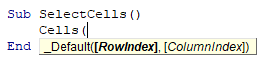
This type of syntax is called R1C1 syntax as opposed to the A1 syntax of a column letter and then a row number which is used when using the Range Object in Excel VBA.
Therefore, to select cell C3 we can type the following code:
Cells(3, 4).Selectthis will move the Excel pointer to cell C4 in your worksheet.
If we wish to use the cells function to populate a specific cell with some text, and then format the cell, we can write some code like this example below:
Sub PopulateCell()
   Cells(2, 2) = "Sales Analysis for 2022"
   Cells(2, 2).Font.Bold = True
   Cells(2, 2).Font.Name = "Arial"
   Cells(2, 2).Font.Size = 12
End Sub
This will populate cell B2 with text and then format the cell.
Worksheet.Cells
If we wish to select the entire worksheet using the Cells Function, we can type the following:
Worksheets("Sheet1").Cells.SelectThis will select all the cells in Sheet 1 in the same way that pressing CTRL + A on the keyboard would do so.
Range.Cells
We can also use the cells function to refer to a specific cell within a range of cells.
Range("A5:B10").Cells(2, 2).SelectThis will actually refer to the cell that has the address of B6 in the original range (A5:B10) as B6 is in the second row and second column of that range.
Looping through a Range with the Cells Function
Now that we understand the Cells Function, we can use it to perform some tasks in VBA Loops.
For example, if we want to format a range of cells depending on their value, we can loop through the range using the cells function.
Sub FormatCells()
   Dim x As Integer
   For x = 1 To 10
      If Cells(x, 1) > 5 Then
         Cells(x, 1).Interior.Color = vbRed
      End If
   Next x
End Sub
This code will start at cell A1 and loop through to cell A10, changing the background color to red if the value in the cell is greater than 5.
If we wish to take this to another level, to loop through columns as well as rows, we can add in a further loop to the code to increase the columns that the loops looks at.
Sub FormatCells()
   Dim x As Integer
   Dim y As Integer
   For x = 1 To 10
      For y = 1 To 5
         If Cells(x, y) > 5 Then
            Cells(x, y).Interior.Color = vbRed
         End If
      Next y
   Next x
End Sub
Now the loop will start at cell A5 but will continue all the way through to cell E10.
We can also use the Cells function to loop through a specific range of cells
Sub LoopThrouRange()
   Dim rng As Range
   Dim x As Integer
   Dim y As Integer
   Set rng = Range("B2:D8")
   For x = 1 To 7
      For y = 1 To 3
         If rng.Cells(x, y) > 5 Then
            rng.Cells(x, y).Interior.Color = vbRed
         End If
      Next y
   Next x
End Sub
This loop would only look inside the range B2:D8, and then loop through the rows and columns of that particular range. Remember that when the range is supplied to the Cells Function, the Cells Function will only look within that range and not at the entire worksheet.
VBA Coding Made Easy
Stop searching for VBA code online. Learn more about AutoMacro — A VBA Code Builder that allows beginners to code procedures from scratch with minimal coding knowledge and with many time-saving features for all users!

Learn More!
Cells are actually cells of the worksheet and in VBA when we refer to cells as a range property we are actually referring to the exact cells, in other words, cell is used with range property and the method of using cells property is as follows Range(.Cells(1,1)) now cells (1,1) means the cell A1 the first argument is for the row and second is for the column reference.
VBA Cell References
You don’t need any special introduction about what is a VBA cell. In VBA concepts, cells are also the same, no different from normal excel cells. Follow this article to have more knowledge of the VBA cells concept.
Table of contents
- VBA Cell References
- What is VBA Range & VBA Cell?
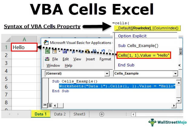
- The Formula of CELLS Property in VBA
- #1 – How to Use CELLS Property in VBA?
- #2 – How to Use CELLS Property with Range Object?
- #3 – Cells Property with Loops
- Things to Remember in VBA Cells
- Recommended Articles
What is VBA Range & VBA Cell?
I am sure this is the question running in your mind right now. In VBA, Range is an object, but Cell is a property in an excel sheet. In VBA, we have two ways of referencing a cell object one through Range, and another one is through Cells.
For example, if you want to reference cell C5, you can use two methods to refer to the cell C5.
Using Range Method: Range (“C5”)
Using Cells Method: Cells (5, 3)
Similarly, if you want to insert value “Hi” to C5 cell, then you can use the below code.
Using Range Method: Range (“C5”).Value = “Hi”
Using Cells Method: Cells (5, 3).Value = “Hi”
Now, if you want to select multiple cells, we can only select through the Range object. For example, if I want to select cells from A1 to A10, below is the code.
Code: Range (“A1: A10”).Select
But unfortunately, we can only reference one cellCell reference in excel is referring the other cells to a cell to use its values or properties. For instance, if we have data in cell A2 and want to use that in cell A1, use =A2 in cell A1, and this will copy the A2 value in A1.read more at a time by using CELLS property. We can use Cells with a Range object like the below.
Range (“A1: C10”).Cells(5,2) mean in the range A1 to C10 fifth row and second column i.e., B5 cell.
The Formula of CELLS Property in VBA
Take a look at the formula of CELLS property.

- Row Index: This nothing but which row we are referencing.
- Column Index: This nothing but which column we are referencing.
- Cells (1, 1) means A1 cell, Cells (2, 1) means A2 cell, Cells (1, 2) means B1 cell.
- Cells (2, 2) means B2 cell, Cells (10, 3) means C10 cell, Cells (15, 5) means E15 cell.
#1 – How to Use CELLS Property in VBA?
Now I will teach you how to use these CELLS property in VBA.
You can download this VBA Cells Excel Template here – VBA Cells Excel Template
Assume you are working in the sheet name called Data 1, and you want to insert a value “Hello” to the cell A1.
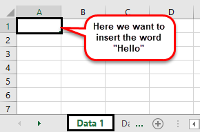
The Below code would do that for you.
Sub Cells_Example()
Cells(1, 1).Value = "Hello"
End Sub
Result:
Now I will go to the sheet name called Data 2 and will run the code. Even there, it will insert the word “Hello.”
Actually, we can combine the CELLS property with a particular sheet name as well. To refer a particular sheet, use the WORKSHEET object.
Worksheets(“Data 1”).Cells(1,1).Value = “Hello”
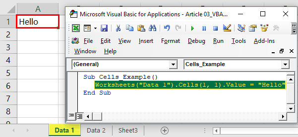
This will insert the word “Hello” to the sheet “Data 1” irrespective of which sheet you are in.
#2 – How to Use CELLS Property with Range Object?
Actually, we can use CELLS property with a RANGE object. For example, look at the below code.
Range("C2:E8").Cells(1, 1).Select

For better understanding, I have entered a few numbers in the excel sheet.
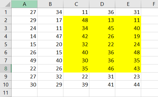
The above code Range(“C2:E8”).Cells(1, 1).Select says in the range C2 to E8 select the first cell. Run this code and see what happens.
Sub Cells_Example()
Range("C2:E8").Cells(1, 1).Select
End Sub

It has selected the cell C2. But Cells (1, 1) means A1 cell, isn’t it?
The reason it has selected the cell C2 because using range object, we have insisted on the range as C2 to E8, so Cells property treats the range from C2 to E8, not from regular A1 cell. In this example, C2 is the first row and first column, so Cells (1, 1).select means C2 cell.
Now I will change the code to Range(“C2: E8”).Cells(3, 2).Select and see what happens.
Run this code and check which cell actually it will select.
Sub Cells_Example()
Range("C2:E8").Cells(3, 2).Select
End Sub
It has selected the cell D4 i.e., No 26. Cells (3,2) mean starting from C2 cell moved down by 3 rows and move 2 columns to the right i.e., D4 cell.
#3 – Cells Property with Loops
CELLS property with loops has a very good relationship in VBA. Let’s look at the example of inserting serial numbers from 1 to 10 using FOR LOOP. Copy and paste the below code to your module.
Sub Cells_Example()
Dim i As Integer
   For i = 1 To 10
     Cells(i, 1).Value = i
     Next i
End Sub
Here I have declared the variable I as an integer.
Then I have applied FOR LOOP with I = 1 to 10 i.e., and the loop needs to run 10 times.
Cells(i,1).value = i
This means that when the loop first runs, the value of “I” will be 1, so wherever the value of “I” is 1 i.e., Cell(1,1).value = 1
When the loop returns the value of “I” for the second time, it is 2, so wherever the value of “I” is, it is 2. i.e., Cell(2,1).value = 2
This loop will run for 10 times and insert I value from A1 to A10.
Things to Remember in VBA Cells
- CELLS is property, but the RANGE is an Object. We can use property with objects but not object to the property.
- When the range is supplied, cells will consider only that range, not the regular range.
- Cells (1, 2) is B1 cell, similarly Cells (1, ”B”) is also B1 cell.
Recommended Articles
This has been a Guide to VBA Cells. Here we learn how to use VBA Cell Reference Property with Range Object along with practical examples and downloadable excel templates. Below you can find some useful excel VBA articles –
- Select Cell in VBAVBA select cell assists the users to pick any particular cell using various methods like Macro recorder, range object, select statement, CELLS property and cell reference.read more
- Use VBA Range Function
- VLookup in Excel VBAThe functionality of VLOOKUP in VBA is similar to that of VLOOKUP in a worksheet, and the method of using VLOOKUP in VBA is through an application. Method WorksheetFunctionread more
- Excel VBA Range CellsThe range property of VBA is used to refer to any data, cells, or selection. It is an inbuilt property that allows us to access any part of the worksheet. Using the range property for a single cell-like range is referred to as range cells.read more