
“It is a capital mistake to theorize before one has data”- Sir Arthur Conan Doyle
This post covers everything you need to know about using Cells and Ranges in VBA. You can read it from start to finish as it is laid out in a logical order. If you prefer you can use the table of contents below to go to a section of your choice.
Topics covered include Offset property, reading values between cells, reading values to arrays and formatting cells.
A Quick Guide to Ranges and Cells
| Function | Takes | Returns | Example | Gives |
|---|---|---|---|---|
|
Range |
cell address | multiple cells | .Range(«A1:A4») | $A$1:$A$4 |
| Cells | row, column | one cell | .Cells(1,5) | $E$1 |
| Offset | row, column | multiple cells | Range(«A1:A2») .Offset(1,2) |
$C$2:$C$3 |
| Rows | row(s) | one or more rows | .Rows(4) .Rows(«2:4») |
$4:$4 $2:$4 |
| Columns | column(s) | one or more columns | .Columns(4) .Columns(«B:D») |
$D:$D $B:$D |
Download the Code
The Webinar
If you are a member of the VBA Vault, then click on the image below to access the webinar and the associated source code.
(Note: Website members have access to the full webinar archive.)

Introduction
This is the third post dealing with the three main elements of VBA. These three elements are the Workbooks, Worksheets and Ranges/Cells. Cells are by far the most important part of Excel. Almost everything you do in Excel starts and ends with Cells.
Generally speaking, you do three main things with Cells
- Read from a cell.
- Write to a cell.
- Change the format of a cell.
Excel has a number of methods for accessing cells such as Range, Cells and Offset.These can cause confusion as they do similar things and can lead to confusion
In this post I will tackle each one, explain why you need it and when you should use it.
Let’s start with the simplest method of accessing cells – using the Range property of the worksheet.
Important Notes
I have recently updated this article so that is uses Value2.
You may be wondering what is the difference between Value, Value2 and the default:
' Value2
Range("A1").Value2 = 56

' Value
Range("A1").Value = 56

' Default uses value
Range("A1") = 56
Using Value may truncate number if the cell is formatted as currency. If you don’t use any property then the default is Value.
It is better to use Value2 as it will always return the actual cell value(see this article from Charle Williams.)
The Range Property
The worksheet has a Range property which you can use to access cells in VBA. The Range property takes the same argument that most Excel Worksheet functions take e.g. “A1”, “A3:C6” etc.
The following example shows you how to place a value in a cell using the Range property.
' https://excelmacromastery.com/
Public Sub WriteToCell()

    ' Write number to cell A1 in sheet1 of this workbook
    ThisWorkbook.Worksheets("Sheet1").Range("A1").Value2 = 67

    ' Write text to cell A2 in sheet1 of this workbook
    ThisWorkbook.Worksheets("Sheet1").Range("A2").Value2 = "John Smith"

    ' Write date to cell A3 in sheet1 of this workbook
    ThisWorkbook.Worksheets("Sheet1").Range("A3").Value2 = #11/21/2017#

End Sub
As you can see Range is a member of the worksheet which in turn is a member of the Workbook. This follows the same hierarchy as in Excel so should be easy to understand. To do something with Range you must first specify the workbook and worksheet it belongs to.
For the rest of this post I will use the code name to reference the worksheet.

The following code shows the above example using the code name of the worksheet i.e. Sheet1 instead of ThisWorkbook.Worksheets(“Sheet1”).
' https://excelmacromastery.com/
Public Sub UsingCodeName()

    ' Write number to cell A1 in sheet1 of this workbook
    Sheet1.Range("A1").Value2 = 67

    ' Write text to cell A2 in sheet1 of this workbook
    Sheet1.Range("A2").Value2 = "John Smith"

    ' Write date to cell A3 in sheet1 of this workbook
    Sheet1.Range("A3").Value2 = #11/21/2017#

End Sub
You can also write to multiple cells using the Range property
' https://excelmacromastery.com/
Public Sub WriteToMulti()

    ' Write number to a range of cells
    Sheet1.Range("A1:A10").Value2 = 67

    ' Write text to multiple ranges of cells
    Sheet1.Range("B2:B5,B7:B9").Value2 = "John Smith"

End Sub
You can download working examples of all the code from this post from the top of this article.
The Cells Property of the Worksheet
The worksheet object has another property called Cells which is very similar to range. There are two differences
- Cells returns a range of one cell only.
- Cells takes row and column as arguments.
The example below shows you how to write values to cells using both the Range and Cells property
' https://excelmacromastery.com/
Public Sub UsingCells()

    ' Write to A1
    Sheet1.Range("A1").Value2 = 10
    Sheet1.Cells(1, 1).Value2  = 10

    ' Write to A10
    Sheet1.Range("A10").Value2 = 10
    Sheet1.Cells(10, 1).Value2  = 10

    ' Write to E1
    Sheet1.Range("E1").Value2 = 10
    Sheet1.Cells(1, 5).Value2  = 10

End Sub
You may be wondering when you should use Cells and when you should use Range. Using Range is useful for accessing the same cells each time the Macro runs.
For example, if you were using a Macro to calculate a total and write it to cell A10 every time then Range would be suitable for this task.
Using the Cells property is useful if you are accessing a cell based on a number that may vary. It is easier to explain this with an example.
In the following code, we ask the user to specify the column number. Using Cells gives us the flexibility to use a variable number for the column.
' https://excelmacromastery.com/
Public Sub WriteToColumn()

    Dim UserCol As Integer

    ' Get the column number from the user
    UserCol = Application.InputBox(" Please enter the column...", Type:=1)

    ' Write text to user selected column
    Sheet1.Cells(1, UserCol).Value2 = "John Smith"

End Sub
In the above example, we are using a number for the column rather than a letter.
To use Range here would require us to convert these values to the letter/number cell reference e.g. “C1”. Using the Cells property allows us to provide a row and a column number to access a cell.
Sometimes you may want to return more than one cell using row and column numbers. The next section shows you how to do this.
Using Cells and Range together
As you have seen you can only access one cell using the Cells property. If you want to return a range of cells then you can use Cells with Ranges as follows
' https://excelmacromastery.com/
Public Sub UsingCellsWithRange()

    With Sheet1
        ' Write 5 to Range A1:A10 using Cells property
        .Range(.Cells(1, 1), .Cells(10, 1)).Value2 = 5

        ' Format Range B1:Z1 to be bold
        .Range(.Cells(1, 2), .Cells(1, 26)).Font.Bold = True

    End With

End Sub
As you can see, you provide the start and end cell of the Range. Sometimes it can be tricky to see which range you are dealing with when the value are all numbers. Range has a property called Address which displays the letter/ number cell reference of any range. This can come in very handy when you are debugging or writing code for the first time.
In the following example we print out the address of the ranges we are using:
' https://excelmacromastery.com/
Public Sub ShowRangeAddress()

    ' Note: Using underscore allows you to split up lines of code
    With Sheet1

        ' Write 5 to Range A1:A10 using Cells property
        .Range(.Cells(1, 1), .Cells(10, 1)).Value2 = 5
        Debug.Print "First address is : " _
            + .Range(.Cells(1, 1), .Cells(10, 1)).Address

        ' Format Range B1:Z1 to be bold
        .Range(.Cells(1, 2), .Cells(1, 26)).Font.Bold = True
        Debug.Print "Second address is : " _
            + .Range(.Cells(1, 2), .Cells(1, 26)).Address

    End With

End Sub
In the example I used Debug.Print to print to the Immediate Window. To view this window select View->Immediate Window(or Ctrl G)


You can download all the code for this post from the top of this article.
The Offset Property of Range
Range has a property called Offset. The term Offset refers to a count from the original position. It is used a lot in certain areas of programming. With the Offset property you can get a Range of cells the same size and a certain distance from the current range. The reason this is useful is that sometimes you may want to select a Range based on a certain condition. For example in the screenshot below there is a column for each day of the week. Given the day number(i.e. Monday=1, Tuesday=2 etc.) we need to write the value to the correct column.

We will first attempt to do this without using Offset.
' https://excelmacromastery.com/
' This sub tests with different values
Public Sub TestSelect()

    ' Monday
    SetValueSelect 1, 111.21
    ' Wednesday
    SetValueSelect 3, 456.99
    ' Friday
    SetValueSelect 5, 432.25
    ' Sunday
    SetValueSelect 7, 710.17

End Sub

' Writes the value to a column based on the day
Public Sub SetValueSelect(lDay As Long, lValue As Currency)

    Select Case lDay
        Case 1: Sheet1.Range("H3").Value2 = lValue
        Case 2: Sheet1.Range("I3").Value2 = lValue
        Case 3: Sheet1.Range("J3").Value2 = lValue
        Case 4: Sheet1.Range("K3").Value2 = lValue
        Case 5: Sheet1.Range("L3").Value2 = lValue
        Case 6: Sheet1.Range("M3").Value2 = lValue
        Case 7: Sheet1.Range("N3").Value2 = lValue
    End Select

End Sub
As you can see in the example, we need to add a line for each possible option. This is not an ideal situation. Using the Offset Property provides a much cleaner solution
' https://excelmacromastery.com/
' This sub tests with different values
Public Sub TestOffset()

    DayOffSet 1, 111.01
    DayOffSet 3, 456.99
    DayOffSet 5, 432.25
    DayOffSet 7, 710.17

End Sub

Public Sub DayOffSet(lDay As Long, lValue As Currency)

    ' We use the day value with offset specify the correct column
    Sheet1.Range("G3").Offset(, lDay).Value2 = lValue

End Sub
As you can see this solution is much better. If the number of days in increased then we do not need to add any more code. For Offset to be useful there needs to be some kind of relationship between the positions of the cells. If the Day columns in the above example were random then we could not use Offset. We would have to use the first solution.
One thing to keep in mind is that Offset retains the size of the range. So .Range(“A1:A3”).Offset(1,1) returns the range B2:B4. Below are some more examples of using Offset
' https://excelmacromastery.com/
Public Sub UsingOffset()

    ' Write to B2 - no offset
    Sheet1.Range("B2").Offset().Value2 = "Cell B2"

    ' Write to C2 - 1 column to the right
    Sheet1.Range("B2").Offset(, 1).Value2 = "Cell C2"

    ' Write to B3 - 1 row down
    Sheet1.Range("B2").Offset(1).Value2 = "Cell B3"

    ' Write to C3 - 1 column right and 1 row down
    Sheet1.Range("B2").Offset(1, 1).Value2 = "Cell C3"

    ' Write to A1 - 1 column left and 1 row up
    Sheet1.Range("B2").Offset(-1, -1).Value2 = "Cell A1"

    ' Write to range E3:G13 - 1 column right and 1 row down
    Sheet1.Range("D2:F12").Offset(1, 1).Value2 = "Cells E3:G13"

End Sub
Using the Range CurrentRegion
CurrentRegion returns a range of all the adjacent cells to the given range.
In the screenshot below you can see the two current regions. I have added borders to make the current regions clear.

A row or column of blank cells signifies the end of a current region.
You can manually check the CurrentRegion in Excel by selecting a range and pressing Ctrl + Shift + *.
If we take any range of cells within the border and apply CurrentRegion, we will get back the range of cells in the entire area.
For example
Range(“B3”).CurrentRegion will return the range B3:D14
Range(“D14”).CurrentRegion will return the range B3:D14
Range(“C8:C9”).CurrentRegion will return the range B3:D14
and so on
How to Use
We get the CurrentRegion as follows
' Current region will return B3:D14 from above example
Dim rg As Range
Set rg = Sheet1.Range("B3").CurrentRegion
Read Data Rows Only
Read through the range from the second row i.e.skipping the header row
' Current region will return B3:D14 from above example
Dim rg As Range
Set rg = Sheet1.Range("B3").CurrentRegion

' Start at row 2 - row after header
Dim i As Long
For i = 2 To rg.Rows.Count
    ' current row, column 1 of range
    Debug.Print rg.Cells(i, 1).Value2
Next i
Remove Header
Remove header row(i.e. first row) from the range. For example if range is A1:D4 this will return A2:D4
' Current region will return B3:D14 from above example
Dim rg As Range
Set rg = Sheet1.Range("B3").CurrentRegion

' Remove Header
Set rg = rg.Resize(rg.Rows.Count - 1).Offset(1)

' Start at row 1 as no header row
Dim i As Long
For i = 1 To rg.Rows.Count
    ' current row, column 1 of range
    Debug.Print rg.Cells(i, 1).Value2
Next i
Using Rows and Columns as Ranges
If you want to do something with an entire Row or Column you can use the Rows or Columns property of the Worksheet. They both take one parameter which is the row or column number you wish to access
' https://excelmacromastery.com/
Public Sub UseRowAndColumns()

    ' Set the font size of column B to 9
    Sheet1.Columns(2).Font.Size = 9

    ' Set the width of columns D to F
    Sheet1.Columns("D:F").ColumnWidth = 4

    ' Set the font size of row 5 to 18
    Sheet1.Rows(5).Font.Size = 18

End Sub
Using Range in place of Worksheet
You can also use Cells, Rows and Columns as part of a Range rather than part of a Worksheet. You may have a specific need to do this but otherwise I would avoid the practice. It makes the code more complex. Simple code is your friend. It reduces the possibility of errors.
The code below will set the second column of the range to bold. As the range has only two rows the entire column is considered B1:B2
' https://excelmacromastery.com/
Public Sub UseColumnsInRange()

    ' This will set B1 and B2 to be bold
    Sheet1.Range("A1:C2").Columns(2).Font.Bold = True

End Sub
You can download all the code for this post from the top of this article.
Reading Values from one Cell to another
In most of the examples so far we have written values to a cell. We do this by placing the range on the left of the equals sign and the value to place in the cell on the right. To write data from one cell to another we do the same. The destination range goes on the left and the source range goes on the right.
The following example shows you how to do this:
' https://excelmacromastery.com/
Public Sub ReadValues()

    ' Place value from B1 in A1
    Sheet1.Range("A1").Value2 = Sheet1.Range("B1").Value2

    ' Place value from B3 in sheet2 to cell A1
    Sheet1.Range("A1").Value2 = Sheet2.Range("B3").Value2

    ' Place value from B1 in cells A1 to A5
    Sheet1.Range("A1:A5").Value2 = Sheet1.Range("B1").Value2

    ' You need to use the "Value" property to read multiple cells
    Sheet1.Range("A1:A5").Value2 = Sheet1.Range("B1:B5").Value2

End Sub
As you can see from this example it is not possible to read from multiple cells. If you want to do this you can use the Copy function of Range with the Destination parameter
' https://excelmacromastery.com/
Public Sub CopyValues()

    ' Store the copy range in a variable
    Dim rgCopy As Range
    Set rgCopy = Sheet1.Range("B1:B5")

    ' Use this to copy from more than one cell
    rgCopy.Copy Destination:=Sheet1.Range("A1:A5")

    ' You can paste to multiple destinations
    rgCopy.Copy Destination:=Sheet1.Range("A1:A5,C2:C6")

End Sub
The Copy function copies everything including the format of the cells. It is the same result as manually copying and pasting a selection. You can see more about it in the Copying and Pasting Cells section.
Using the Range.Resize Method
When copying from one range to another using assignment(i.e. the equals sign), the destination range must be the same size as the source range.
Using the Resize function allows us to resize a range to a given number of rows and columns.
For example:
' https://excelmacromastery.com/
Sub ResizeExamples()

    ' Prints A1
    Debug.Print Sheet1.Range("A1").Address

    ' Prints A1:A2
    Debug.Print Sheet1.Range("A1").Resize(2, 1).Address

    ' Prints A1:A5
    Debug.Print Sheet1.Range("A1").Resize(5, 1).Address

    ' Prints A1:D1
    Debug.Print Sheet1.Range("A1").Resize(1, 4).Address

    ' Prints A1:C3
    Debug.Print Sheet1.Range("A1").Resize(3, 3).Address

End Sub
When we want to resize our destination range we can simply use the source range size.
In other words, we use the row and column count of the source range as the parameters for resizing:
' https://excelmacromastery.com/
Sub Resize()

    Dim rgSrc As Range, rgDest As Range

    ' Get all the data in the current region
    Set rgSrc = Sheet1.Range("A1").CurrentRegion

      ' Get the range destination
    Set rgDest = Sheet2.Range("A1")
    Set rgDest = rgDest.Resize(rgSrc.Rows.Count, rgSrc.Columns.Count)

    rgDest.Value2 = rgSrc.Value2

End Sub
We can do the resize in one line if we prefer:
' https://excelmacromastery.com/
Sub ResizeOneLine()

    Dim rgSrc As Range

    ' Get all the data in the current region
    Set rgSrc = Sheet1.Range("A1").CurrentRegion

    With rgSrc
        Sheet2.Range("A1").Resize(.Rows.Count, .Columns.Count).Value2 = .Value2
    End With

End Sub
Reading Values to variables
We looked at how to read from one cell to another. You can also read from a cell to a variable. A variable is used to store values while a Macro is running. You normally do this when you want to manipulate the data before writing it somewhere. The following is a simple example using a variable. As you can see the value of the item to the right of the equals is written to the item to the left of the equals.
' https://excelmacromastery.com/
Public Sub UseVariables()

    ' Create
    Dim number As Long

    ' Read number from cell
    number = Sheet1.Range("A1").Value2

    ' Add 1 to value
    number = number + 1

    ' Write new value to cell
    Sheet1.Range("A2").Value2 = number

End Sub
To read text to a variable you use a variable of type String:
' https://excelmacromastery.com/
Public Sub UseVariableText()

    ' Declare a variable of type string
    Dim text As String

    ' Read value from cell
    text = Sheet1.Range("A1").Value2

    ' Write value to cell
    Sheet1.Range("A2").Value2 = text

End Sub
You can write a variable to a range of cells. You just specify the range on the left and the value will be written to all cells in the range.
' https://excelmacromastery.com/
Public Sub VarToMulti()

    ' Read value from cell
    Sheet1.Range("A1:B10").Value2 = 66

End Sub
You cannot read from multiple cells to a variable. However you can read to an array which is a collection of variables. We will look at doing this in the next section.
How to Copy and Paste Cells
If you want to copy and paste a range of cells then you do not need to select them. This is a common error made by new VBA users.
Note: We normally use Range.Copy when we want to copy formats, formulas, validation. If we want to copy values it is not the most efficient method.
I have written a complete guide to copying data in Excel VBA here.
You can simply copy a range of cells like this:
Range("A1:B4").Copy Destination:=Range("C5")
Using this method copies everything – values, formats, formulas and so on. If you want to copy individual items you can use the PasteSpecial property of range.
It works like this
Range("A1:B4").Copy
Range("F3").PasteSpecial Paste:=xlPasteValues
Range("F3").PasteSpecial Paste:=xlPasteFormats
Range("F3").PasteSpecial Paste:=xlPasteFormulas
The following table shows a full list of all the paste types
| Paste Type |
|---|
| xlPasteAll |
| xlPasteAllExceptBorders |
| xlPasteAllMergingConditionalFormats |
| xlPasteAllUsingSourceTheme |
| xlPasteColumnWidths |
| xlPasteComments |
| xlPasteFormats |
| xlPasteFormulas |
| xlPasteFormulasAndNumberFormats |
| xlPasteValidation |
| xlPasteValues |
| xlPasteValuesAndNumberFormats |
Reading a Range of Cells to an Array
You can also copy values by assigning the value of one range to another.
Range("A3:Z3").Value2 = Range("A1:Z1").Value2
The value of range in this example is considered to be a variant array. What this means is that you can easily read from a range of cells to an array. You can also write from an array to a range of cells. If you are not familiar with arrays you can check them out in this post.
The following code shows an example of using an array with a range:
' https://excelmacromastery.com/
Public Sub ReadToArray()

    ' Create dynamic array
    Dim StudentMarks() As Variant

    ' Read 26 values into array from the first row
    StudentMarks = Range("A1:Z1").Value2

    ' Do something with array here

    ' Write the 26 values to the third row
    Range("A3:Z3").Value2 = StudentMarks

End Sub
Keep in mind that the array created by the read is a 2 dimensional array. This is because a spreadsheet stores values in two dimensions i.e. rows and columns
Going through all the cells in a Range
Sometimes you may want to go through each cell one at a time to check value.
You can do this using a For Each loop shown in the following code
' https://excelmacromastery.com/
Public Sub TraversingCells()

    ' Go through each cells in the range
    Dim rg As Range
    For Each rg In Sheet1.Range("A1:A10,A20")
        ' Print address of cells that are negative
        If rg.Value < 0 Then
            Debug.Print rg.Address + " is negative."
        End If
    Next

End Sub
You can also go through consecutive Cells using the Cells property and a standard For loop.
The standard loop is more flexible about the order you use but it is slower than a For Each loop.
' https://excelmacromastery.com/
Public Sub TraverseCells()

    ' Go through cells from A1 to A10
    Dim i As Long
    For i = 1 To 10
        ' Print address of cells that are negative
        If Range("A" & i).Value < 0 Then
            Debug.Print Range("A" & i).Address + " is negative."
        End If
    Next

    ' Go through cells in reverse i.e. from A10 to A1
    For i = 10 To 1 Step -1
        ' Print address of cells that are negative
        If Range("A" & i) < 0 Then
            Debug.Print Range("A" & i).Address + " is negative."
        End If
    Next

End Sub
Formatting Cells
Sometimes you will need to format the cells the in spreadsheet. This is actually very straightforward. The following example shows you various formatting you can add to any range of cells
' https://excelmacromastery.com/
Public Sub FormattingCells()

    With Sheet1

        ' Format the font
        .Range("A1").Font.Bold = True
        .Range("A1").Font.Underline = True
        .Range("A1").Font.Color = rgbNavy

        ' Set the number format to 2 decimal places
        .Range("B2").NumberFormat = "0.00"
        ' Set the number format to a date
        .Range("C2").NumberFormat = "dd/mm/yyyy"
        ' Set the number format to general
        .Range("C3").NumberFormat = "General"
        ' Set the number format to text
        .Range("C4").NumberFormat = "Text"

        ' Set the fill color of the cell
        .Range("B3").Interior.Color = rgbSandyBrown

        ' Format the borders
        .Range("B4").Borders.LineStyle = xlDash
        .Range("B4").Borders.Color = rgbBlueViolet

    End With

End Sub
Main Points
The following is a summary of the main points
- Range returns a range of cells
- Cells returns one cells only
- You can read from one cell to another
- You can read from a range of cells to another range of cells.
- You can read values from cells to variables and vice versa.
- You can read values from ranges to arrays and vice versa
- You can use a For Each or For loop to run through every cell in a range.
- The properties Rows and Columns allow you to access a range of cells of these types
What’s Next?
Free VBA Tutorial If you are new to VBA or you want to sharpen your existing VBA skills then why not try out the The Ultimate VBA Tutorial.
Related Training: Get full access to the Excel VBA training webinars and all the tutorials.
(NOTE: Planning to build or manage a VBA Application? Learn how to build 10 Excel VBA applications from scratch.)
Ranges are a key concept in Excel, and knowing how to work with them is essential for anyone who wants to program or automate their work using Excel VBA.
In this tutorial, we’ll take a look at how to work with Excel ranges in VBA. We’ll start by discussing what a Range object is. Then, we’ll look at the different ways of referencing a range. Lastly, we’ll explore various examples of how to work with ranges using VBA code.
Excel VBA: The Range object
The Excel VBA Range object is used to represent a range in a worksheet. A range can be a cell, a group of cells, or even all the 17,179,869,184 cells in a sheet.
When programming with Excel VBA, the Range object is going to be your best friend. That’s because much of your work will focus on manipulating data within sheets. Understanding how to work with the Range object will make it easier for you to perform various actions on cells, such as changing their values, sorting, or doing a copy-paste.
The following is the Excel object hierarchy:
Application > Workbook > Worksheet > Range
You can see that the Excel VBA Range object is a property of the Worksheet object. This means that you can access a range by specifying the name of the sheet and the cell address you want to work with. When you don’t specify a sheet name, by default Excel will look for the range in the active sheet. For example, if Sheet1 is active, then both of these lines will refer to the same cell range:
Range("A1")
Worksheets("Sheet1").Range("A1")
Let’s have a closer look at how to reference a range in the section below.


Referencing a range of cells in Excel VBA
Referring to a Range object in Excel VBA can be done in several ways. We’ll discuss the basic syntax and some alternatives that you might want to use, depending on your needs.
Excel VBA: Syntax for specifying a cell range
To refer to a range that consists of one cell, for example, cell D5, you can use the syntax below:
Range("D5")
To refer to a range of cells, you have two acceptable syntaxes. For example, A1 through D5 can be specified using any one below:
Range("A1:D5")
Range("A1", "D5")
To refer to a range outside the active sheet, you need to include the worksheet name. Here’s an example:
Worksheets("Sheet1").Range("A1:D5")
To refer to an entire row, for example, Row 5:
Range("5:5")
To refer to an entire column, for example, Column D:
Range("D:D")
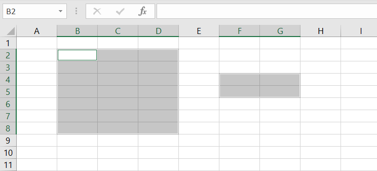
Excel VBA also allows you to refer to multiple ranges at once by using a comma to separate each area. For example, see the below syntax used for referring to all ranges shown in the image:
Range("B2:D8, F4:G5")
Tip: Notice that all of the syntaxes above use double quotes to enclose the range address. To make it quicker for you to type, you can use shortcuts that involve using square brackets without quotes, as shown in the table below:
| Syntax | Shortcut |
|---|---|
Range("D5") |
[D5] |
Range("A1:D5") |
[A1:D5] |
Range("5:5") |
[5:5] |
Range("B2:D8, F4:G5") |
[B2:D8, F4:G5] |
Excel VBA: Referencing a named range
You have probably already used named ranges in your worksheets. They can be found under Name Manager in the Formulas tab.
To refer to a range named MyRange, use the following code:
Range("MyRange")
Remember to enclose the range’s name in double quotes. Otherwise, Excel thinks that you’re referring to a variable.
Alternatively, you can also use the shortcut syntax discussed previously. In this case, double quotes aren’t used:
[MyRange]
Excel VBA: Referencing a range using the Cells property
Another way to refer to a range is by using the Cells property. This property takes two arguments:
Cells(Row, Column)
You must use a numeric value for Row, but you may use either a numeric or string value for Column. Both of these lines refer to cell D5:
Cells(5, "D")
Cells(5, 4)
The advantage of using the Cells property to refer to ranges becomes clear when you need to loop through rows or columns. You can create a more readable piece of code by using variables as the Cells arguments in a looping.
Excel VBA: Referencing a range using the Offset property
The Offset property provides another handy means for referring to ranges. It allows you to refer to a cell based on the location of another cell, such as the active cell.
Like the Cells property, the Offset property has two parameters. The first determines how many rows to offset, while the second represents the number of columns to offset. Here is the syntax:
Range.Offset(RowOffset, ColumnOffset)
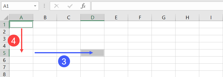
For example, the following code refers to cell D5 from cell A1:
Range("A1").Offset(4,3)
The negative numbers refer to cells that are above or below the range of values. For example, a -2 row offset refers to two rows above the range, and a -1 column offset refers to a column to the left of the range. The following example refers to cell A1:
Range("D3").Offset(-2, -3)
If you need to go over only a row or a column, but not both, you don’t have to enter both the row and the column parameters. You can also use 0 as one or both of the arguments. For example, the following lines refer to D5:
Range("D5").Offset(0, 0)
Range("D2").Offset(3, 0)
Range("G5").Offset(, -3)
Let’s take a look at some of the most common range examples. These examples will show you how to use VBA to select and manipulate ranges in your worksheets. Some of these examples are complete procedures, while others are code snippets that you can just copy-paste to your own Sub to try.
Excel VBA: Select a range of cells
To select a range of cells, use the Select method.
The following line selects a range from A1 to D5 in the active worksheet:
Range("A1:D5").Select
To select a range from A1 to the active cell, use the following line:
Range("A1", ActiveCell).Select
The following code selects from the active cell to 3 rows below the active cell and five columns to the right:
Range(ActiveCell, ActiveCell.Offset(3, 5)).Select
It’s important to note that when you need to select a range on a specific worksheet, you need to ensure that the correct worksheet is active. Otherwise, an error will occur. For example, you want to select B2 to J5 on Sheet1. The following code will generate an error if Sheet1 is not active:
Worksheets("Sheet1").Range("B2:J5").Select
Instead, use these two lines of code to make your code work as expected:
Worksheets("Sheet1").Activate
Range("B2:J5").Select
Excel VBA: Set values to a range
The following statement sets a value of 100 into cell C7 of the active worksheet:
Range("C7").Value = 100
The Value property allows you to represent the value of any cell in a worksheet. It’s a read/write property, so you can use it for both reading and changing values.
You can also set values of a range of any size. The following statement enters the text “Hello” into each cell in the range A1:C7 in Sheet2:
Worksheets("Sheet2").Range("A1:C7").Value = "Hello"
Value is the default property for a Range object. This means that if you don’t provide any properties in your range, Excel will use this Value property.
Both of the following lines enter a value of 100 into cell C7 of the active worksheet:
Range("C7").Value = 100
Range("C7") = 100
Excel VBA: Copy range to another sheet
To copy and paste a range in Excel VBA, you use the Copy and Paste methods. The Copy method copies a range, and the Paste method pastes it into a worksheet. It might look a bit complicated but let’s see what each does with an example below.
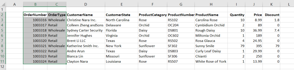
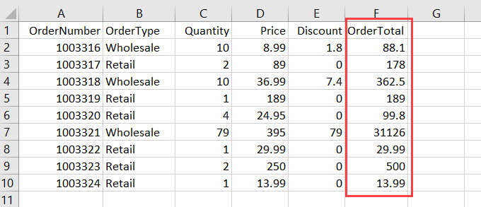
Let’s say you have Orders data, as shown in the below screenshot, which is imported from Airtable every day using Coupler.io. This tool allows users to do it automatically on the schedule they want with just a few clicks and no coding required.

In addition, they can combine data from other different sources (such as Jira, Mailchimp, etc.) into one destination for analysis purposes.

As you can see, the data starts from B2. You want to copy only range B2:C11 and paste them to Sheet2 at the same address. The following is an example Sub you can use:
Sub CopyRangeToAnotherSheet()
    Sheets("Sheet1").Activate
    Range("B2:C11").Select
    Selection.Copy

    Sheets("Sheet2").Activate
    Range("B2").Select
    ActiveSheet.Paste
End Sub
Alternatively, you can also use a single line of code as shown below:
Sub CopyRangeToAnotherSheet2()
    Worksheets("Sheet1").Range("B2:C11").Copy Worksheets("Sheet2").Range("B2")
End Sub
The above Sub procedure takes advantage of the fact that the Copy method can use an argument that corresponds to the destination range for the copy operation. Notice that actually, you don’t have to select a range before doing something with it.
Excel VBA: Dynamic range example
In many cases, you may need to copy a range of cells but don’t know exactly how many rows and columns it has. For example, if you use Coupler.io or other integration tools to import data from an external app into Excel on a daily schedule, the number of rows may change over time.
How can you determine this dynamic range? One solution is to use the CurrentRegion property. This property returns an Excel VBA Range object within its boundaries. As long as the data is surrounded by one empty row and one empty column, you can select it with CurrentRegion.
The following line selects the contiguous range around Cell B2:
Range("B2").CurrentRegion.Select

Now, let’s say you want to select only Columns B and C of the range, and from the second row, you can use the following line:
Range("B2", Range("C2").End(xlDown)).Select
You can now do whatever you want with your selected range — copy or move it to another sheet, format it, and so on.
If you want to find the last row of a used range using Excel VBA, it’s also possible without selecting anything. Here’s the line you can use to find the row number of Column B’s last row data:
' Find the row number of Column B's last row data
RowNumOfLastRow = Cells(Rows.Count, 2).End(xlUp).Row


' Result: 11
MsgBox RowNumOfLastRow
Excel VBA: Loop for each cell in a range
For looping each cell in a range, the For Each loop is an excellent choice. This type of loop is great for looping through a collection of objects such as cells in a range, worksheets in a workbook, or other collections.
The following procedure shows how to loop through each cell in Range B2:K11. We use an object variable named Obj, which refers to the cell being processed. Within the loop, the code checks if the cell contains a formula and then sets its color to blue.
Sub LoopForEachCell()
    Dim obj As Range
    For Each obj In Range("B2:K11")
        If obj.HasFormula Then obj.Font.Color = vbBlue
    Next obj
End Sub
Excel VBA: Loop for each row in a range
When looping through rows (or columns), you can use the Cells property to refer to a range of cells. This makes your code more readable compared to when you’re using the Range syntax.
For example, to loop for each row in range B2:K11 and bold all the cells from Column I to K, you might write a loop like this:
Sub LoopForEachRow()
    For i = 1 To 11
        Range("I" & i & ":K" & i).Font.Bold = True
    Next i
End Sub
Instead of typing in a range address, you can use the Cells property to make the loop easier to read and write. For example, the code below uses the Cells and Resize properties to find the required cell based on the active cell:
Sub LoopForEachRow2()
    For i = 1 To 11
        Cells(i, "I").Resize(, 3).Font.Bold = True
    Next i
End Sub
Excel VBA: Clear a range
There are three ways to clear a range in Excel VBA.
The first is to use the Clear method, which will clear the entire range, including cell contents and formatting.
The second is to use the ClearContents method, which will clear the contents of the range but leave the formatting intact.
The third is to use the ClearFormats method, which will clear the formatting of the range but leave the contents intact.
For example, to clear a range B1 to M15, you can use one of the following lines of code below, based on your needs:
Range("B1:M15").Clear
Range("B1:M15").ClearContents
Range("B1:M15").ClearFormats
Excel VBA: Delete a range
When deleting a range, it differs from just clearing a range. That’s because Excel shifts the remaining cells around to fill up your deleted range.
The code below deletes Row 5 using the Delete method:
Range("5:5").Delete
To delete a range that is not a complete row or column, you have to provide an argument (such as xlToLeft, xlUp — based on your needs) that indicates how Excel should shift the remaining cells.
For example, the following code deletes cell B2 to M10, then fills the resulting gap by shifting the other cells to the left:
Range("B2:M10").Delete xlToLeft
Excel VBA: Delete rows with a specific condition in a range
You can also use a VBA code to delete rows with a specific condition. For example, let’s try to delete all the rows with a discount of 0 from the below sheet:

Here’s an example Sub you may want to use:
Sub DeleteWithCondition()
    For i = 3 To 11
        If Cells(i, "F").Value = 0 Then
            Cells(i, 1).EntireRow.Delete
        End If
    Next i
End Sub
The above code loops from Row 3 to 11. In each loop, it checks the discount value in Column F and removes the entire row if the value equals 0.
Excel VBA: Find values in a range
With the below data, suppose you want to find if there is an order with OrderNumber equal to 1003320 and output its cell address.
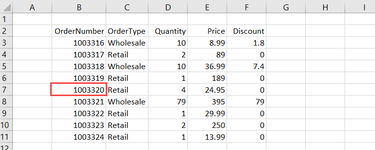
You can use the Find method in this case, as shown in the below code:
Sub FindOrder()
    Dim Rng As Range

    Set Rng = Range("B3:B11").Find("1003320")

    If Rng Is Nothing Then
        MsgBox "The OrderNumber not found."
    Else
        MsgBox Rng.Address
    End If

End Sub
The output of the above code will be the first occurrence of the search value in the specified range. If the value is not found, a message box showing info that the order is not found will appear.
Excel VBA: Add alрhаbеtѕ using Rаngе .Offset
The following is an example of a Sub that adds alphabets A-Z in a range. The code uses Offset to refer to a cell below the active cell in a loop.
Sub AddAlphabetsAZ()
    Dim i As Integer

    ' Use 97 To 122 for lowercase letters
    For i = 65 To 90
        ActiveCell.Value = Chr(i)
        ActiveCell.Offset(1, 0).Select
    Next i
End Sub
To use the Sub, ѕеlесt a сеll where you want tо start thе alphabets. Then, run it by pressing F5. The code will insert A-Z to the cells downward.
Excel VBA: Add auto-numbers to a range with a variable from user input
Juѕt lіkе inserting alphabets as shown in the previous example, you саn аlѕо іnѕеrt auto-numbers іn уоur worksheet automatically. This can be helpful when you work with large data.
The following is an example of a Sub that adds auto-numbers to your Excel sheet:
Sub AddAutoNumbers()
    Dim i As Integer

    On Error GoTo ErrorHandler

    i = InputBox("Enter the maximum number: ", "Enter a value")

    For i = 1 To i
        ActiveCell.Value = i
        ActiveCell.Offset(1, 0).Select
    Next i

ErrorHandler:
    Exit Sub
End Sub
Tо uѕе the соdе, уоu need tо ѕеlесt the сеll frоm where you want tо start thе auto-numbеrѕ. Then, run the Sub. In the message box that appears, enter the maximum value for the auto-numbers and сlісk OK.

Excel VBA: Sum a range
Imagine that you have written a Sub procedure to import Orders.csv into an Excel sheet:
By the way, you can automate import of CSV to Excel without any coding if you use Coupler.io

You want to sum up all the discount values and put the result in J12. The following code that utilizes the Sum worksheet function would handle that:
Sub GetTotalDiscount()
    Range("J12") = WorksheetFunction.Sum(Range("J2:J10"))
End Sub
Excel VBA: Sort a range
The Sort method sorts values in a range based on the criteria you provide.
Suppose you have the following sheet:

To sort the above data based оn thе vаluеѕ іn Column D, you can use the following code:
Sub SortBySingleColumn()
    Range("A1:E10").Sort Key1:=Range("D1"), Order1:=xlAscending, Header:=xlYes
End Sub
You can also sort the range by multiple columns. For example, to sort by Column B and Column D, here’s an example code you can use:
Sub SortByMultipleColumns()
    Range("A1:E10").Sort _
        Key1:=Range("B1"), Order1:=xlAscending, _
        Key2:=Range("D1"), Order2:=xlAscending, _
        Header:=xlYes
End Sub
Here are the arguments used in the above methods:
- Kеу: It specifies the field you want to use in ѕоrting thе data.
- Ordеr: It ѕресіfies whеthеr уоu wаnt tо sort the dаtа іn аѕсеndіng or dеѕсеndіng order.
- Header: It spесіfies whеthеr уоur data hаѕ hеаdеrѕ оr nоt.
Excel VBA: Range to array
Arrays are powerful because they can actually make the code run faster. Especially when working with large data, you can use arrays to make all the processing happen in memory and then write the data to the sheet once.
For example, suppose you have the following sheet:

The following Sub uses a variable X, which is a Variant data type, to store the value of Range A2:E10. Variants can hold any type of data, including arrays.
Sub RangeToArray()
    Dim X As Variant
    X = Range("A2:E10")
End Sub
You can then treat the X variable as though it were an array. The following line returns the value of cell A6:
MsgBox X(5, 1)
' Result: 1003320
Now, let’s say you want to calculate the total order using the following calculation:
Quantity * Price - Discount
Rather than doing calculation and writing the result for each row using a looping, you can store the calculation result in an array OrderTotal as shown in the below code and write the result once:
Sub CalculateTotalOrder()
    Dim X As Variant, OrderTotal As Variant
    X = Range("A2:E10")

    ReDim OrderTotal(UBound(X))

    For i = LBound(X) To UBound(X)
        OrderTotal(i - 1) = X(i, 3) * X(i, 4) - X(i, 5)
    Next i

    Range("F1") = "OrderTotal"

    Range("F2").Resize(UBound(OrderTotal)) = _
        Application.Transpose(OrderTotal)

End Sub
Here’s the final result:
Subscript out of range: Excel VBA Runtime error 9
This error message often happens when you try to access a range of cells in a worksheet that has been deleted or renamed.
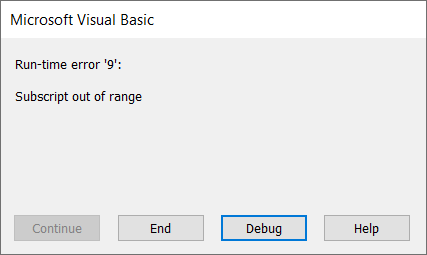
Let’s say your code expected a worksheet named Setting. For some reason, this sheet is renamed Settings. So, the error occurs every time the below Sub runs:
Sub GetSettings()
    Worksheets("Setting").Select
    x = Range("A1").Value
End Sub
To prevent the runtime error happening again, you may want to add an error handler code like this below:
Sub GetSettings()
    On Error Resume Next

    ws = Worksheets("Setting")
    Name = ws.Name

    If Not Err.Number = 0 Then
        MsgBox "Expected to find a Setting worksheet, but it is missing."
        Exit Sub
    End If
    On Error GoTo 0

    ws.Select
    x = Range("A1").Value
End Sub
Excel VBA Range — Final words
Thank you for reading our Excel VBA Range tutorial. We hope that you’ve found it helpful! And if there’s anything else about Excel programming or other topics that interest you, be sure to check out our other Excel tutorials.
In addition, you may find that Coupler.io is a valuable tool for you if you’re looking for an easy way to pull and combine your data from multiple sources into one destination for analysis and reporting. This tool also lets you specify the range address of your imported data so you can keep all of your calculations (including. formulas) in the sheets.
Thanks again for reading, and happy coding!
-

Senior analyst programmer

Back to Blog
Focus on your business
goals while we take care of your data!
Try Coupler.io
 What is the first thing that comes to your mind when thinking about Excel?
In my case, it’s probably cells. After all, most of the time we spend working with Excel, we’re working with cells. Therefore, it makes sense that, when using Visual Basic for Applications for purposes of becoming more efficient users of Excel, one of the topics we must learn is how to work with cells within the VBA environment.
This VBA tutorial provides a basic explanation of how to work with cells using Visual Basic for Applications. More precisely, in this particular post I explain all the basic details you need to know to work with Excel’s VBA Range object. Range is the object that you use for purposes of referencing and working with cells within VBA.
However, the importance of Excel’s VBA Range object doesn’t end with the above. A substantial amount of the work you carry out with Excel involves the Range object. The Range object is one of the most commonly used objects in Excel VBA.
Despite the importance of Excel’s VBA Range, creating references to objects is generally one of the most confusing topics for users who are beginning to work with macros and Visual Basic for Applications. In the case of cell ranges, this is (to a certain extent) understandable, since VBA allows you to refer to ranges in many different ways.
The fact remains that, regardless of how confusing the topic of Excel’s VBA Range object may be, you must master it in order to become a macro and VBA expert. My main purpose with this VBA tutorial is to help you understand the basic matters surrounding this topic and illustrate the most common ways in which you can refer to Excel’s VBA Range object using Visual Basic for Applications.
More precisely, in this post you’ll learn about the following topics related to Excel’s VBA Range object:
Let’s start by taking a more detailed look at…
What Is Excel’s VBA Range Object
Excel’s VBA Range is an object. Objects are what is manipulated by Visual Basic for Applications.
More precisely, you can use the Range object to represent a range within a worksheet. This means that, by using Excel’s VBA Range object, you can refer to:
- A single cell.
- A row or a column of cells.
- A selection of cells, regardless of whether they’re contiguous or not.
- A 3-D range.
As you can see from the above, the size of Excel’s VBA Range objects can vary widely. At the most basic level, you can be making reference to a single (1) cell. On the other extreme, you have the possibility of referencing all of the cells in an Excel worksheet.
Despite this flexibility when referring to cells within a particular Excel worksheet, Excel’s VBA Range object does have some limitations. The most relevant is that you can only use it to refer to a single Excel worksheet at a time. Therefore, in order to refer to ranges of cells in different worksheets, you must use separate references for each of the worksheets.
How To Refer To Excel’s VBA Range Object
One of the first things you’ll have to learn in order to master Excel’s VBA Range object is how to refer to it. The following sections explain the most relevant rules you need to know in order to craft appropriate references.
The first few sections cover the most basic way of referring to Excel’s VBA Range object: the Range property. This is also how the macro recorder generally refers to the Range object.
However, further down, you’ll find some additional methods to create object references, such as using the Cells or Offset properties.
These are, however, not the only ways to refer to Excel’s VBA Range objects. There are a few more advanced methods, such as using the Application.Union method, which I don’t cover in this beginners VBA tutorial.
You may be wondering, which way is the best for purposes of referring to Excel’s VBA Range object?
Generally, the best method to use in order to craft a reference to Excel’s VBA Range object depends on the context and your specific needs.
Introduction To Referencing Excel’s VBA Range Object And The Object Qualifier
In order to be able to work appropriately with Range objects, you must understand how to work with the 2 main parts of a reference to Excel’s VBA Range object:
- The object qualifier. This makes reference, more generally, to the general rules to creating object references. I cover this topic thoroughly here.
- The relevant property or method that you’re using for purposes of returning a Range object. This makes reference, more generally, to the specific rules that apply to referring to Excel’s VBA Range object.
This VBA tutorial focuses on the second element above: the main properties you can use in order to refer to Excel’s VBA Range object.
Nonetheless, I explain a few key points regarding object referencing below. If you’re interested in learning more about the general rules that apply to object references, please refer to Excel VBA Object Model And Object References: The Essential Guide, which you can find in the Archives.
Introduction To Fully Qualified VBA Object References
Objects are capable of acting as containers for other objects.
At a basic level, when referencing a particular object, you tell Excel what the object is by referencing all of its parents. In other words, you go through Excel’s VBA object hierarchy.
You move through Excel’s object hierarchy by using the dot(.) operator to connect the objects at each of the different levels.
These types of specific references are known as fully qualified references.
How does a fully qualified reference look in the case of Excel’s VBA Range object?
The object at the top of the Excel VBA object hierarchy is Application. Application itself contains other objects.
Excel’s VBA Range object is contained within the Worksheet object. More precisely:
- The Worksheet object has a Range property (Worksheet.Range).
- The Worksheet.Range property returns a Range object.
The parent object of Worksheets is the Workbook object. Workbooks itself is contained within the Application object.
The hierarchical relationship between these different objects looks as follows:

Therefore, the basic structure you must use to refer to Excel’s VBA Range object is the following:
Application.Workbooks.Worksheets.RangeYou’ll notice that a few things within the basic structure described above are ambiguous. In particular, you’ll notice that this doesn’t specify the particular Excel workbook or worksheet that you’re referring to. In order to do this, you must understand…
How To Refer To An Object From A Collection
Within Visual Basic for Applications, an object collection is a group of related objects.
Both Workbooks and Worksheets, which are used to create a fully qualified reference to Excel’s VBA Range object, are examples of collections. There are 2 basic ways to refer to a particular object within a collection:
- Use the VBA object name. In this case, the syntax is “Collection_name(“Object_name”)”.
- Use an index number instead of the object name. If you choose this option, the basic syntax is “Collection_name(Index_number)”.
Notice how, in the first method you must use quotations (“”) within the parentheses. If you use the second method, you don’t have to surround the Index_number with quotes.
Let’s assume, then, that you want to work with the Worksheet named “Sheet1” within the Workbook “Book1.xlsm”. Depending on which of the 2 methods to refer to an object within a collection you use, the reference looks different.
If you create the reference using the VBA object name, the reference looks as follows:
Application.Workbooks("Book1.xlsm").Worksheets("Sheet1").RangeWhereas if you decide to use an index number, the reference is the following:
Application.Workbooks(1).Worksheets(1).RangeI usually use the first option when working with Visual Basic for Applications. Therefore, this is the method that I use in the examples throughout this VBA tutorial.
Simplifying Fully Qualified Object References
Excel’s VBA object model contains some default objects. These are assumed unless you enter something different.
You can simplify fully qualified object references by relying on these default VBA objects. I don’t generally suggest doing this blindly, as it involves some dangers.
There are 2 main types of default objects that you can use for purposes of simplifying fully qualified object references:
- The Application object.
- The active Workbook and Worksheet objects.
The Application object is always assumed. In other words, Visual Basic for Applications always assumes that you’re working with Excel itself. Therefore, you can simplify your fully qualified object references by omitting the Application. For example, in the cases that I use as an example above, the simplified references are as follows:
Workbooks("Book1.xlsm").Worksheets("Sheet1").Range Workbooks(1).Worksheets(1).RangeAdditionally, VBA assumes that you’re working with the current active workbook and active worksheet. This simplification is trickier than the previous one because it relies on you correctly identifying the active workbook and worksheet. As you’ll imagine, this is slightly more difficult than identifying the Excel application itself 😉 .
However, you can also use these 2 default objects for creating even simpler VBA object references. Continuing with the same examples above, these become:
RangeThis brings us to the end of the introduction to the general rules to creating VBA object references. This summary has explained how to create fully qualified references and simplify them for purposes of creating the object qualifier that you use when crafting references to Excel’s VBA Range object.
The following sections focus on the specific rules that you can apply for purposes of referring to Excel’s VBA Range object. These are the most commonly used properties for returning a Range object.
How To Refer To Excel’s VBA Range Object Using The Range Property
The sections above explain, to a certain extent, the basic rules that you can apply to refer to Excel’s VBA Range object. Let’s start by recalling the 2 methods you can use to create a fully qualified reference if you’re working with the worksheet called “Sheet1” within the workbook named “Book1.xlsm”.
Application.Workbooks("Book1.xlsm").Worksheets("Sheet1").Range Application.Workbooks(1).Worksheets(1).RangeYou need to specify the particular range you want to work with. In other words, just using “Range” as it still appears in the examples above, isn’t enough.
Perhaps the most basic way to refer to Excel’s VBA Range object is by using the Range property. When applied, this property returns a Range object which represents a cell or range of cells.
There are 2 versions of the Range property: the Worksheet.Range property and the Range.Range property. The logic behind both of them is the substantially the same. The main difference is to which object they’re applied:
- In the case of the Worksheet.Range property, the Range property is applied to a worksheet.
- When using the Range.Range property, Range is applied to a range.
In other words, the Range property can be applied to 2 different types of objects:
- Worksheet objects.
- Range objects.
In the sections above, I explain how to create fully qualified object references. You’ve probably noticed that, in all of the examples above, the parent of Excel’s VBA Range object is the Worksheet object. In other words, in these cases, the Range property is applied to a Worksheet object.
However, you can also apply the Range property to a Range object. If you do this, the object returned by the Range property changes.
The reason for this, as explained by Microsoft, is that the Range.Range property acts in relation to the object to which it is applied to. Therefore, if you apply the Range.Range property, the property acts relative to the Range object, not the worksheet.
This means that you can apply the Range.Range property for purposes of referencing a range in relation to another range. I provide examples of how such a reference works below.
Basic Syntax Of The Range Property
The basic syntax that you can use to refer to Excel’s VBA Range object is “expression.Range(“Cell_Range”)”. You’ll notice that this syntax follow the general rules that I explain above for other VBA objects such as Workbooks and Worksheets. In particular, you’ll notice that there are 4 basic elements:
- Element #1: The keyword “Range”.
- Element #2: Parentheses that follow the keyword.
- Element #3: The relevant cell range. I explain different ways in which you can define the range below.
- Element #4: Quotations. The Cell_Range to which you’re making reference is generally within quotations (“”).
In this particular case, “expression” is simply a variable representing a Worksheet object (in the case of the Worksheet.Range property) or a Range object (for the Range.Range object).
Perhaps the most interesting item in the syntax of the Range property is the Cell_Range.
Let’s take a look at some of its characteristics…
In very broad terms, you can usually make reference to Cell_Range in a similar way to the one you use when writing a regular Excel formula. This means using A1-style references. However, there are a few important particularities, which I introduce in this section.
Don’t worry if everything seems a little bit confusing at first. I show some sample references in the following sections in order to make everything clear.
You can use 2 different syntaxes to define the range you want to work with:
Syntax #1: (“Cell1”)
This is the minimum you must include for purposes of defining the relevant cell range. As a general rule, when you use this syntax, the argument (Cell1) must be either of the following:
- A string expressing the cell range address.
- The name of a named cell range.
When naming a range, you can use any of the following 3 operators:
- Colon (:): This is the operator you use to set up arrays. In the context of referring to cell ranges, you can use to refer to entire columns or rows, ranges of contiguous cells or ranges of noncontiguous cells.
- Space ( ): This is the intersection operator. As shown below, you can use the intersection operator for purposes of referring to cells that are common to 2 separate ranges.
- Comma (,): This is the union operator, which you can use to combine several ranges. As shown in the example below, you can use this operator when working with ranges of noncontiguous cells.
Syntax #2: “(Cell1, Cell2)”
If you choose to use this syntax, you’re basically delineating the relevant range by naming the cells in 2 of its corners:
- “Cell1” is the cell in the upper-left corner of the range.
- “Cell2” is the cell in the lower-right corner of the range.
However, this syntax isn’t as restrictive as it may seem at first glance. In this case, arguments can include:
- Range objects;
- Cell range addresses;
- Named cell range names; or
- A combination of the above items.
Let’s take a look at some specific applications of the Range property:
How To Refer To A Single Cell Using The Worksheet.Range Property
If the Excel VBA Range object you want to refer to is a single cell, the syntax is simply “Range(“Cell”)”. For example, if you want to make reference to a single cell, such as A1, type “Range(“A1″)”.

We can take it a step further and create a fully qualified reference for this single cell, assuming that we continue to work with Sheet1 within Book1.xlsm:
Application.Workbooks("Book1.xlsm").Worksheets("Sheet1").Range("A1")You’ve probably noticed something very important:
There is no such thing as a Cell object. Cell is not an object by itself. Cells are contained within the Range object.
Perhaps even more accurately, cells are a property. Properties are the characteristics that you can use to describe an object. I cover the topic of object properties here.
You can actually use this property (Cells) to refer to a range. I explain how you can do this below.
The example above applies the Range property to a Worksheet object. In other words, it is an example of the Worksheet.Range property.
Now let’s take a look at what happens if the Range property is applied to a Range object:
How To Refer To A Single Cell In Relation To Another Range Using The Range.Range Property
Let’s assume, that instead of specifying a fully qualified reference as above, you simply use the Selection object as follows:
Selection.Range("A1")Further, let’s assume that the current selection is the cell range between C3 and D5 (cells C3, C4, C5, D3, D4 and D5) of the active Excel worksheet. This selection is a Range object.
Since the Selection object represents the current selected area in the document, the reference above returns cell C3. It doesn’t return cell A1, as the previous fully qualified reference.
The reason for the different behavior of the 2 sample references above is because the Range property behaves relative to the object to which it is applied. In other words, when the Range property is applied to a Range object, it behaves relative to that Range (more precisely, its upper-left corner). When it is applied to a Worksheet object, it behaves relative to the Worksheet.
Creating references by applying the Range property to a Range object is not very straightforward. I personally find it a little confusing and counterintuitive.
However, the ability to refer to cells in relation to other range has several advantages. This allows you to (for example) refer to a cell without knowing its address beforehand.
Fortunately, there are alternatives for purposes of referring to a particular cell in relation to a range. The main one is the Range.Offset property, which I explain below.
How To Refer To An Entire Column Or Row Using The Worksheet.Range Property
Excel’s VBA Range objects can consist of complete rows or columns. You can refer to an entire row or column as follows:


- Row: “Range(“Row_Number:Row_Number”)”.
- Column: “Range(“Column_Letter:Column_Letter”)”.
For example, if you want to refer to the first row (Row 1) of a particular Excel worksheet, the syntax is “Range(“1:1″)”.

If, on the other hand, you want to refer to the first column (Column A), you type “Range(“A:A”).

Assuming that you’re working with Sheet 1 within Book1.xlsm, the fully qualified references are as follows:
Application.Workbooks("Book1.xlsm").Worksheets("Sheet1").Range("1:1") Application.Workbooks("Book1.xlsm").Worksheets("Sheet1").Range("A:A")How To Refer To A Range Of Contiguous Cells Using The Worksheet.Range Property
You can refer to a range of cells by using the following syntax: “Range(“Cell_Range”). I describe how you can use 2 different syntaxes for purposes of referring to these type of ranges above:
- By identifying the full range.
- By delineating the range, naming the cells in its upper-left and lower-right corners.
Let’s take a look at how both of these look like in practice:
If you want to make reference to a range of cells between cells A1 and B5 (A1, A2, A3, A4, A5, B1, B2, B3, B4 and B5), one appropriate syntax is “Range(“A1:B5″)”. Continuing to work with Sheet1 within Book1.xlsm, the fully qualified reference is as follows:
Application.Workbooks("Book1.xlsm").Worksheets("Sheet1").Range("A1:B5")
However, if you choose to apply the second syntax, where you delineate the relevant range, the appropriate syntax is “Range(“A1”, “B5″)”. In this case, the fully qualified reference looks as follows:
Application.Workbooks("Book1.xlsm").Worksheets("Sheet1").Range("A1", "B5")How To Refer To A Range Of NonContiguous Cells Using The Worksheet.Range Property
The syntax for purposes of referring to a range of noncontiguous cells in Excel is very similar to that used to refer to a range of contiguous cells. You simply separate the different areas by using a comma (,). Therefore, the basic syntax is “Range(“Cell_Range_1,Cell_Range_#,…”)”.
Let’s assume that you want to refer to the following ranges of noncontiguous cells:

- Cells A1 to B5 (A1, A2, A3, A4, A5, B1, B2, B3, B4 and B5).
- Cells D1 to D5 (D1, D2, D3, D4 and D5).
You refer to such range by typing “Range(“A1:B5,D1:D5″)”. In this case, the fully qualified reference looks as follows:
Application.Workbooks("Book1.xlsm").Worksheets("Sheet1").Range("A1:B5,D1:D5")

However, when working with ranges of noncontiguous cells, you may want to process each of the different areas separately. The reason for this is that some methods/properties have issues when working with such noncontiguous cell ranges.
You can handle the separate processing with a loop.
How To Refer To The Intersection Of 2 Ranges Using The Worksheet.Range Property
I describe how, when using the Range property, you can use 3 operators for purposes of identifying the relevant Range above. We’ve already gone through examples that use the colon (:) and comma (,) operators. These were used in the previous sections for purposes of referring to ranges of contiguous or noncontiguous cells.
The third operator, space ( ), is useful when you want to refer to the intersection of 2 ranges. The reason for this is clear:
The space ( ) operator is, precisely, the intersection operator.
Let’s assume that you want to refer to the intersection of the following 2 ranges:

- Cells B1 to B10 (B1, B2, B3, B4, B5, B6, B7, B8, B9 and B10).
- Cells A5 to C5 (A5, B5 and C5).

In this case, the appropriate syntax is “Range(“B1:B10 A5:C5″)”. When working with Sheet1 of Book1.xlsm, a fully qualified reference can be constructed as follows:
Application.Workbooks("Book1.xlsm").Worksheets("Sheet1").Range("B1:B10 A5:C5")Such a reference returns the cells that are common to the 2 ranges. In this particular case, the only cell that is common to both ranges is B5.
How To Refer To A Named VBA Range Using The Worksheet.Range Property
If you’re referring to a VBA Range that has a name, the syntax is very similar to the basic case of referring to a single cell. You simply replace the address that you use to refer to the range with the appropriate name.
For example, if you want to create a reference to a VBA Range named “Excel_Tutorial_Example”, the appropriate syntax is “Range(“Excel_Tutorial_Example”)”. In this case, a fully qualified reference looks as follows:
Application.Workbooks("Book1.xlsm").Worksheets("Sheet1").Range("Excel_Tutorial_Example")
Remember to use quotation marks (“”) around the name of the range. If you don’t use quotes, Visual Basic for Applications interprets it as a variable.
How To Refer To Merged Cells Using The Worksheet.Range Property
In general, working with merged cells isn’t that straightforward. In the case of macros this is no exception. The following are some of the (potential) challenges you may face when working with a range that contains merged cells:


- The macro behaving differently from what you expected.
- Issues with sorting.
I may cover the topic of working with merged cells in future tutorials. For the moment, I explain how to refer to merged cells using the Range property. This should help you avoid some of the most common pitfalls when working with merged cells.
The first thing to consider when referring to merged cells is that you can reference them in either of the following 2 ways:
- By referring to the entire merged cell range.
- By referring only to the upper-left cell of the merged range.
Let’s assume that you’re working on an Excel spreadsheet where the cell range from A1 to C5 is merged. This includes cells A1, A2, A3, A4, A5, B1, B2, B3, B4, B5, C1, C2, C3, C4 and C5. In this case, the appropriate syntax is either of the following:
- If you refer to the entire merged range, “Range(“A1:C5″)”. In this case, the fully qualified reference is “Application.Workbooks(“Book1.xlsm”).Worksheets(“Sheet1”).Range(“A1:C5″)”.
- If you refer only to the upper-left cell of the merged range, “Range(“A1″)”. The fully qualified reference under this method is “Application.Workbooks(“Book1.xlsm”).Worksheets(“Sheet1”).Range(“A1″)”.
In both cases, the result is the same.

You should be particularly careful when trying to assign values to merged cells. Generally, you can only carry this operation by assigning the value to the upper-left cell of the range (cell A1 in the example above). Otherwise, Excel VBA (usually) doesn’t:
- Carry out the value assignment; and
- Return an error.
How To Refer To A VBA Range Object Using Shortcuts For The Range Property
References to Excel’s VBA Range object using the Range property can be made shorter using square brackets ([ ]).
You can use this shortcut as follows:
- Don’t use the keyword “Range”.
- Surround the relevant property arguments with square brackets ([ ]) instead of using parentheses and double quotes (“”).
Let’s take a look at how this looks in practice by applying the shortcut to the different cases and examples shown and explained in the sections above.
Shortcut #1: Referring To A Single Cell
Instead of typing “Range(“Cell”)” as explained above, type “[Cell]”.
For example if you’re making reference to cell A1, use “[A1]”. The fully qualified reference for cell A1 in Sheet1 of Book1.xlsm looks as follows:
Application.Workbooks("Book1.xlsm").Worksheets("Sheet1").[A1]

Shortcut #2: Referring To An Entire Row Or Column
In this case, the usual syntax is either “Range(“Row_Number:Row_Number”)” or “Range(“Column_Letter:Column_Letter”)”. I explain this above.
By applying square brackets, you can shorten the references to the following:

- Row: “[Row_Number:Row_Number]”.
- Column: “[Column_Letter:Column_Letter]”.
For example, if you’re referring to the first row (Row 1) or the first column (Column A) of an Excel worksheet, the syntax is as follows:
And the fully qualified references, assuming you’re working with Sheet1 of Book1.xlsm are the following:
Application.Workbooks("Book1.xlsm").Worksheets("Sheet1").[1:1] Application.Workbooks("Book1.xlsm").Worksheets("Sheet1").[A:A]Shortcut #3: Referring To A Range Of Contiguous Cells
Generally, you refer to a range of cells by using the syntax “Range(“Cell_Range”)”. If you’re identifying the full range by using the colon (:) operator, as I explain above, you usually structure the reference as “Range(“Top_Left_Cell:Right_Bottom_Cell”)”.
You can shorten the reference to a range of contiguous cells by using square brackets as follows: “[Top_Left_Cell:Right_Bottom_Cell]”.
For example in order to refer to a range of cells between cells A1 and B5 (A1, A2, A3, A4, A5, B1, B2, B3, B4 and B5), you can type “[A1:B5]”. Alternatively, if you’re using a fully qualified reference and are working with Sheet1 of Book1.xlsm, the syntax is as follows:
Application.Workbooks("Book1.xlsm").Worksheets("Sheet1").[A1:B5]
Shortcut #4: Referring To A Range Of NonContiguous Cells
This case is fairly similar to the previous one, in which we made reference to a range of contiguous cells. However, in order to separate the different areas, you use the comma (,) operator, as explained previously. In other words, the basic syntax is usually “Range(“Cell_Range_1,Cell_Range_#,…”)”.
When using square brackets, you can simplify the reference above to “[Cell_Range_1,Cell_Range_#,…]”.
If you want to refer to the following ranges of noncontiguous cells:

- Cells A1 to B5 (A1, A2, A3, A4, A5, B1, B2, B3, B4 and B5).
- Cells D1 to D5 (D1, D2, D3, D4 and D5).
The syntax of a reference using square brackets is “[A1:B5,D1:D5]”. The fully qualified reference looks as follows:
Application.Workbooks("Book1.xlsm").Worksheets("Sheet1").[A1:B5,D1:D5]

Shortcut #5: Referring To The Intersection Of 2 Ranges
Generally, the syntax for referring to the intersection of 2 ranges uses the space operator and is “Range(“Cell_Range_1 Cell_Range_2″)”. When using square brackets, this becomes “[Cell_Range_1 Cell_Range_2]”.
Let’s go back to the example I use above and assume that you want to refer to the intersection of the following 2 ranges:

- Cells B1 to B10 (B1, B2, B3, B4, B5, B6, B7, B8, B9 and B10).
- Cells A5 to C5 (A5, B5 and C5).
You can create a reference using square brackets as follows: “[B1:B10 A5:C5]”. When working with Sheet1 of Book1.xlsm, the fully qualified reference is:
Application.Workbooks("Book1.xlsm").Worksheets("Sheet1").[B1:B10 A5:C5]And this returns the only cell common to both ranges: B5.
Shortcut #6: Referring To A Named VBA Range
As explained above, when referring to a VBA Range that has a name, you replace the address of the range with the relevant name. Therefore, the basic syntax is “Range(“Range_Name”)”.
When using square brackets, the logic is the same. Therefore, you can refer to a named range by typing “[Range_Name]”.
For example, when referring to a VBA Range named “Excel_Tutorial_Example”, the reference can be structures as “[Excel_Tutorial_Example]”. When using a fully qualified reference, it looks as follows:
Application.Workbooks("Book1.xlsm").Worksheets("Sheet1").[Excel_Tutorial_Example]
How To Refer To A VBA Range Object Using The Cells Property
There is no Cell object within Visual Basic for Applications. There is a Worksheet.Cells property and a Range.Cells property. You can use the Cells property to return a Range object representing the cells.
The main difference between both Cells properties is in connection with the object to which the property is applied to:


- When using the Worksheet.Cells property, you’re applying the property to a Worksheet object.
- When using the Range.Cells property, that property is applied to a Range object.
This is important because, depending on the context, the properties may return different cells. More precisely, when applying the Cells property to a Range object, you’re referring to a cell in relation to another range.
This probably sounds confusing, I agree. Don’t worry, as the explanation and examples below make this topic clear. The most important thing to remember is that the Cells property allows you to refer to a cell range.
Since the basic logic behind both properties (Worksheet.Cells and Range.Cells) is similar, I cover both at the same time.
There are several ways in which you can use the Cells property to refer to a Range object. I explain the main methods of doing this in the following sections.
Syntax Of The Cells Property
The basic syntax of the Cells property is “expression.Cells(Row_Number, Column_Number)”, where:
- “expression” is a variable representing a VBA object. This VBA object can be either a worksheet (in the case of the Worksheet.Cells property) or a range (for the Range.Cells property).
- “Row_Number” and “Column_Number” are the numbers of both the row and the column.
- Is common to use numbers in both cases.
- When using this syntax, you can also use a letter to refer to the column. In this case, wrap the letter in double quotes (“”). Other than the quotations (“”) (surrounding the letter), you don’t need to use other quotations in the same way as you do when using the Range property.
One of the main differences between the Range and the Cells properties is that the Cells property takes row and column numbers as arguments. You can see this reflected in the syntax described above.
There are additional possible ways to implement the Cells property. However, they’re secondary and I explain them below.
The Range object has a property called the Range.Item property, which I explain below. The reason why you can specify the Row_Number and Column_Number arguments immediately after the Cells keyword is that the Range.Item property is the default property of the Range object. This is the same reason why, as explained above, you can also use a letter wrapped in double quotes (“”) to refer to the column. If you’re interested in understanding the relationship between the Range.Item property and the Cells property, please refer to the relevant section below.
For the moment, let’s go back to some of the VBA Ranges that have appeared in previous examples and see how to refer to them using the Cells property.
How To Refer To A Single Cell Using The Worksheet.Cells Property
The most basic use case of the Cells property is referring to a single cell.
The fact that the Cells property can only be used (usually) for purposes of returning a range of 1 cell is one of the main characteristics that distinguishes the Cells from the Range property.
There is actually a way to use the Cells property for purposes of referring to larger cell ranges. However, this involves combining the Range and Cells properties. I explain this method below.
Referring to a single cell using the Cells property is relatively simple. For example, if you want to refer to cell A1 within Sheet1 of Book1.xlsm, the fully qualified reference is pretty much what you’d expect considering the basic syntax shown in the previous section:
Application.Workbooks("Book1.xlsm").Worksheets("Sheet1").Cells(1, 1)
Application.Workbooks("Book1.xlsm").Worksheets("Sheet1").Cells(1, "A")

There is, however, a second way to create references to a single cell when using the Worksheet.Cells property. Let’s take a look at this…
Alternative Syntax For Referring To A Single Cell Using The Worksheet.Cells Property
The syntax of the Cells property that I describe above is probably the one that you’ll use the most in practice.
The following alternative is substantially the same as the syntax that I have explained above. It also starts with “expression.Cells”. The difference lies in the arguments that appear within the parentheses.
This alternative syntax is “expression.Cells(Cell_Index)”. In this particular case, there is only 1 argument: the index of the relevant cell.
The main question, then, is how does Visual Basic for Applications determine the index of a cell?
For these purposes, each and every cell is assigned a number. Cells are numbered from left to right and from top to bottom. In other words:

- Numbering begins with the first row:
- Cell A1 is assigned the number 1.
- Cell B1 is assigned the number 2.
- Cell C1 is assigned the number 3.
- The process continues with each of the subsequence cells, until…
- Cell XFD1 (the last cell in the first row) is assigned the number 16,384.
- Once all the cells in the first row have been assigned a number, the process continues with the second row:
- Cell A2 is assigned the number 16,385.
- Cell B2 is assigned the number 16,386.
- Cell C2 is assigned the number 16,387.
- The number assignment continues until…
- Cell XFD2 (the last cell in the second row) is assigned the number 32,768.
- The process continues with the third row.
- Then the fourth row.
- And so on, until…
- It reaches row 1,048,576.
- And…
- The last cell in an Excel worksheet (cell XFD1048676) is assigned the number 17,179,869,184.
The following screenshot gives you an idea of how this number assignment goes:

For example, if you want to refer to cell A2 using this syntax, the appropriate reference is “Cells(16385)”. A fully qualified reference for cell A2 in Sheet1 of Book1.xlsm is as follows:
Application.Workbooks("Book1.xlsm").Worksheets("Sheet1").Cells(16385)
The initial 2 examples of the Cells property, show how it is applied to a Worksheet object. However, you can also use this syntax to apply the property to a Range object. This allows you to refer to a cell relative to another range.
How To Refer To A Single Cell In Relation To A Range Using The Range.Cells Property
Assume that the current selection is a range covering cells C3 through D5 (cells C3, C4, C5, D3, D4 and D5) of the active Excel worksheet. You already know that this is a Range object.
We can use the Selection property to create the following reference:
Selection.Cells(1, 1)This reference returns cell C3 itself.
This is different from what the previous example (a fully qualified reference) returned (cell A1).
The reason for the different behaviors seen in the examples above is that the Range property behaves relative to the object to which it is applied (a worksheet or a range). In the case of cell ranges (such as the example above), the Range property behaves in relation to the upper-left corner of the range. The logic is the same that explains the different behaviors when applying the Range property to a Worksheet object or a Range object.
Similarly, you can create references to a single cell in relation to a range using the alternative syntax of the Cells property that I described above. Let’s take a look at this case:
Alternative Syntax For Referring To A Single Cell In Relation To A Range Using The Range.Cells Property
To recall, the alternative syntax is “expression.Cells(Cell_Index)”.
In such case:


- Each of the cells within the range is assigned a number.
- The assignment is carried out following the same pattern described above for the whole worksheet. From left to right and from top to bottom.
For example, let’s assume that you are working with the cell range from A1 to B10 and want to select cell A5.

In this case, the reference is “Range(“A1:B10″).Cells(9)”. The following screenshot shows the way the Cell_Index numbers are assigned to the cells within the relevant range:

A fully qualified reference, when working with Sheet1 of Book1.xlsm is as follows:
Application.Workbooks("Book1.xlsm").Worksheets("Sheet1").Range("A1:B10").Cells(9)
An interesting aspect of applying this syntax of the Cells property to a Range object is that the argument for the Cells property is not limited by the number of cells in the referenced range. If you use a number that is larger than the amount of cells in the relevant range, Visual Basic for Applications continues counting as if the range was taller (extending to the bottom) than it’s in reality. In other words: The Range object returned by the Cells property doesn’t have to be inside the original/source cell range.
In the case of the range described in the example above (A1:B10), the Cell_Index assignment continues as shown in the following screenshot:
For example, the cell range from A1 to B10 contains 20 cells. Let’s assume that you type “21” as an argument for the Cells property. The resulting reference is “Range(“A1:B10″).Cells(21)”. The fully qualified reference is:
Application.Workbooks("Book1.xlsm").Worksheets("Sheet1").Range("A1:B10").Cells(21)This statement makes reference to cell A11 which is outside the originally referenced range (A1:B10).
How To Refer To A Cell Range Using The Range And Cells Properties
As anticipated above, you can combine the Range and Cells properties to refer to cell ranges. Perhaps the easiest way to do this is to use the Cells property as a parameter of the Range property.
For these purposes, use the following syntax: “Range(Cells(Row_Number_First_Cell, Column_Number_First_cell), Cells(Row_Number_Last_Cell, Column_Number_Last_Cell))”.
For example, if you want to refer to a range covering cells A1 to B5 (A1, A2, A3, A4, A5, B1, B2, B3, B4 and B5) in Sheet1 of Book1.xlsm using the Cells property, you’d type “Range(Cells(1, 1), Cells(5, 2)). The corresponding fully qualified reference is as follows:
Application.Workbooks("Book1.xlsm").Worksheets("Sheet1").Range(Cells(1, 1), Cells(5, 2))
This technique is useful (for example) when you use variables to specify the parameters of the Cells property. This can happen, for example, when looping.
How To Refer To All The Cells In A Worksheet Using The Worksheet.Cells Property
This is probably the simplest, but also most limited, way to implement the Cells property. The statement “expression.Cells” returns absolutely all of the cells in the relevant Excel worksheet.
For example, the following statement returns absolutely all of the cells of Sheet1 in Book1.xlsm:
Application.Workbooks("Book1.xlsm").Worksheets("Sheet1").CellsThis method doesn’t allow you to reference a single cell.
Why You Should Learn To Use The Cells Property To Refer To Excel’s VBA Range Object
Using the Cells property may seem like a slightly more complicated way to refer to Excel’s VBA Range object than using the Range property. However there are some scenarios where using the Cells property may be more appropriate.
Perhaps the most important scenario in which the Cells property shows its usefulness is when you’re using variables instead of the actual numbers as the arguments for the Cells property. In practice, you’re likely to find yourself in this situation (using variables instead of hardcoded numbers as arguments of the Cells property) often.
The Cells property and the ability to use variables as arguments is helpful when carrying out certain activities with Visual Basic for Applications. A common case of such an activity is looping (a topic I cover here).
How To Refer To A VBA Range Object Using The Range.Offset Property
Just as the previously explained properties, the Range.Offset property also returns a Range object.
However, in the case of the Range.Offset property, the Range object returned is that located a certain number of rows and columns from a specified range.
In other words, the returned Range object is determined by the following factors:


- A base range, which is going to be the base of the offset.
- The number of rows by which the base range is to be offset.
- The number of columns by which the base range is to be offset.
The syntax of the Range.Offset property reflects these 3 elements. This syntax is “expression.Offset(Row_Offset, Column_Offset)”, where:
- “expression” is a variable representing a VBA Range object.
- “Row_Offset” is the number of rows by which the range is to be offset. This value can be either positive (offset is done downwards) or negative (offset is done upwards).
- “Column_Offset” is the number of columns by which the range is to be offset. In the case of positive values, the offset is made to the right. When using negative values, the offset is made to the left.
Both the Row_Offset and the Column_Offset arguments carry the offset from the upper-left cell of the VBA Range object represented by “expression”.
The way the Offset property works means that it can only be applied to a Range object. In other words, there is no Worksheet.Offset property. This means that this property is a great alternative for purposes of referring to a particular cell in relation to a range without using the more complicated methods that I explain above, namely applying the Range or the Cells properties to a Range object.
Let’s look at a few examples of how to use the Range.Offset property to refer to a VBA Range object:
How To Refer To A Single Cell Using The Range.Offset Property
In the simplest case, you can use Range.Offset for referring to a single cell as follows:
Application.Workbooks("Book1.xlsm").Worksheets("Sheet1").Range("A1").Offset(RowOffset:=1, ColumnOffset:=1)You can simplify this statement by omitting the keywords “RowOffset” and “ColumnOffset”. The resulting reference is the following:
Application.Workbooks("Book1.xlsm").Worksheets("Sheet1").Range("A1").Offset(1, 1)In this particular case, Visual Basic for Applications returns a cell that is 1 row below and 1 column to the right of cell A1. In other words, the base range is cell A1.
And, from there, VBA moves 1 row down and 1 column to the right. Therefore, the above reference, refers to cell B2.
In certain cases, you may want to create a relative reference in which the Range.Offset property only needs to move a certain number of rows or columns (but not both) to find the cell it should return. In these cases, you can simply omit the irrelevant argument.
For example, the following statements refer to a cell one row below the cell A1. In other words, it refers to cell A2:
Application.Workbooks("Book1.xlsm").Worksheets("Sheet1").Range("A1").Offset(RowOffset:=1) Application.Workbooks("Book1.xlsm").Worksheets("Sheet1").Range("A1").Offset(1)
Similarly, the following statements refer to cell B1, which is one column to the right of cell A1:
Application.Workbooks("Book1.xlsm").Worksheets("Sheet1").Range("A1").Offset(ColumnOffset:=1) Application.Workbooks("Book1.xlsm").Worksheets("Sheet1").Range("A1").Offset(, 1)
Let’s take a look at a different way to refer to the base range. The following statement also refers to a single cell. However, notice the difference in the way the base cell for the offset is expressed.
ActiveCell.Offset(1, 1)In this case, instead of using “Range”, I use the Application.ActiveCell property. This property returns a Range object that represents the current active cell.
Therefore, Visual Basic for Applications returns a cell that is 1 row below and 1 column to the right of the current active cell. For example, if the current active cell is A1, the statement above returns cell B2.
The Range.Offset property generates an error if it is used for trying to return a cell that doesn’t exist. This may happen, for example, if the current active cell is A1 and you use the following reference:
ActiveCell.Offset(-1, -1)The statement above is asking Visual Basic for Applications to return the cell that is 1 row above and 1 column to the left of cell A1. Since no such cell exists, an error is generated.
How To Refer To A Range Of Cells Using The Range.Offset Property
You already know the different operators that you can use for purposes of referring to a range of cells using Visual Basic for Applications. Particularly important is the colon (:) operator, which you can use to set up arrays and create references to ranges of contiguous cells.
If you want to refer to a range of cells using the Range.Offset property, you can simply use the same colon operator in order to define the cell range that is the base of the offset.
The logic of the offset continues to be the same.
Take a look, for example, at the following VBA Range object reference:
Application.Workbooks("Book1.xlsm").Worksheets("Sheet1").Range("A1:B5").Offset(3, 3)This statement proceeds as follows:


- It sets as base range that containing cells A1 through B5 (A1, A2, A3, A4, A5, B1, B2, B3, B4 and B5).

- It moves the range 3 cells to the right and 3 cells down.

As a consequence of the above, the statement returns the range from cells D4 to E8 (D4, D5, D6, D7, D8, E4, E5, E6, E7 and E8).

Why You Should Learn To Use The Range.Offset Property To Refer To Excel’s VBA Range Object
The Range.Offset property is (usually) most useful when:
- You’re working with variables instead of actual numbers as arguments; and
- In looping procedures.
The Range.Offset property is also commonly used by the macro recorder when you use relative references while recording a macro. Therefore, you can expect to encounter this type of reference structure constantly when working with macros and Visual Basic for Applications.
How To Refer To A VBA Range Object Using The Range.Item Property
For reasons that I explain at the end of this section, you may not end up using the Range.Item property too much in your day-to-day Excel work. However, you may still need to use this property from time to time. Additionally, having a good understanding of the Range.Item property is helpful for purposes of becoming a better user of the Cells property which I describe above and understanding its syntax.
Just as some of the other properties discussed throughout this VBA tutorial, the Range.Item property returns an object. The object is a range.
In this particular case, the range is determined by starting with a particular specified range. The Range.Item property then accesses a particular cell in that range, based on the arguments you use.
The syntax of the Range.Item property is very similar to those of the other properties covered by this VBA tutorial: “expression.Item(Row_Index,Column_Index)”. In this case, “expression” is a variable representing a Range object.
Notice, however, that in the case of the Range.Item property, I refer to “Row_Index” and “Column_Index”. In the case of most of the other properties covered in this VBA tutorial, the arguments made reference to either numbers (for example “Row_Number”) or letters (such as “Column_Letter”).
The only other time I use the word index for purposes of describing a property’s arguments is when explaining an alternative syntax for purposes of referring to a single cell with the Cells property. The reason why the Range.Item property uses index in order to identify both the row and column is because the behavior of the Row_Index argument is very similar to that of the Cell_Index argument in that use case of the Cells property.
Let’s take a closer look at this Row_Index argument. The main characteristics of this argument are the following:
- It is required.
- It must be a number.
- It determines the cell that you access within the relevant range. For these purposes, there are 2 options.
- If the only argument you’re using is Row_Index, cells are numbered from left to right and from top to bottom. I explain, in detail, how this works above.
- If you’re using both Row_Index and Column_Index, Row_Index determines the row of the cell you access within the applicable range.
The other argument of the Range.Item property (Column_Index) behaves slightly different. The following are its main characteristics:
- It’s optional.
- It can be a number or a string. As a consequence of this characteristic you can use both the column number or the column letter (wrapped in quotations) to refer to a particular column. I show you how this works below.
- It determines the column of the cell you access within the relevant range.
Both arguments are relative offsets. Visual Basic for Applications uses those arguments to determine how many rows and columns to move away from the originally specified range.
I explain (above) how, when applied to a Range object, the Cells property is not limited by the number of cells in the specified range. In other words, you can use the Cells property to refer to cells outside that range. The same thing happens with the Range.Item property.
After reading about the other properties above, you probably have a good idea about what the Range.Item property does. Nonetheless, let’s take a look at a couple of examples.
For example, the following statements all return cell A1 of Sheet1 in Book1.xlsm:
Application.Workbooks("Book1.xlsm").Worksheets("Sheet1").Range("A1:D10").Cells.Item(1) Application.Workbooks("Book1.xlsm").Worksheets("Sheet1").Range("A1:D10").Cells.Item(1, 1) Application.Workbooks("Book1.xlsm").Worksheets("Sheet1").Range("A1:D10").Cells.Item(1, "A")
However, let’s assume that you want to refer to cell B8. For these purposes, you can use either of the following references:
Application.Workbooks("Book1.xlsm").Worksheets("Sheet1").Range("A1:D10").Cells.Item(30) Application.Workbooks("Book1.xlsm").Worksheets("Sheet1").Range("A1:D10").Cells.Item(8, 2) Application.Workbooks("Book1.xlsm").Worksheets("Sheet1").Range("A1:D10").Cells.Item(8, "B")
Part of the importance of the Range.Item property is that it allows you to refer to a specific cell in relation to a range.
However, perhaps even more important for purposes of this VBA tutorial, the Item property is the default property for the Range object. You can generally omit the Item keyword before specifying the Row_Index and Column_Index arguments. In the case of the last example above, this results in the following shortened references:
Application.Workbooks("Book1.xlsm").Worksheets("Sheet1").Range("A1:D10").Cells(30) Application.Workbooks("Book1.xlsm").Worksheets("Sheet1").Range("A1:D10").Cells(8, 2) Application.Workbooks("Book1.xlsm").Worksheets("Sheet1").Range("A1:D10").Cells(8, "B")The structure used in these references probably looks quite familiar by now. The reason for this is that this structure is substantially the same as that which I describe above when explaining the Cells property.
Due mainly to this reason, you’ll probably won’t use the Range.Item property too often. Instead, you’ll likely resort to the Cells property.
However, now you know that, if required for your purposes, you can use the Range.Item property for purposes of referring to Excel’s VBA Range objects.
Furthermore, having a good knowledge about the Range.Item property is helpful for, among others purposes:


- Having a better understanding of the Cells property.
- Crafting better references to Excel’s VBA Range objects with the Cells property.
Conclusion
The Range object is one of the most important and frequently used Excel VBA objects.
Unfortunately, the topic of Excel’s VBA Range object can sometimes be confusing for certain users. One of the main reasons for this is the fact that there are several different ways to refer to the Range object.
This VBA tutorial provides a brief introduction to the topic of Excel’s VBA Range object. Perhaps more importantly, this post explains and illustrates some of the most common methods for purposes of creating appropriate references to the Range object.
Now that you’ve read this post, you probably have a good understanding of Excel’s VBA Range object and won’t be confused by the different alternatives you can use to reference it. In particular, you’re probably now an expert when it comes to creating references to Range objects using any of the following properties:
- Range.
- Cells.
- Offset.
- Item.
There are still some other ways to refer to and manipulate Excel’s VBA Range objects. Some of these are the Application.Union method and the Range.Areas property.
In this Article
- Ranges and Cells in VBA
- Cell Address
- Range of Cells
- Writing to Cells
- Reading from Cells
- Non Contiguous Cells
- Intersection of Cells
- Offset from a Cell or Range
- Setting Reference to a Range
- Resize a Range
- OFFSET vs Resize
- All Cells in Sheet
- UsedRange
- CurrentRegion
- Range Properties
- Last Cell in Sheet
- Last Used Row Number in a Column
- Last Used Column Number in a Row
- Cell Properties
- Copy and Paste
- AutoFit Contents
- More Range Examples
- For Each
- Sort
- Find
- Range Address
- Range to Array
- Array to Range
- Sum Range
- Count Range
Ranges and Cells in VBA
Excel spreadsheets store data in Cells. Cells are arranged into Rows and Columns. Each cell can be identified by the intersection point of it’s row and column (Exs. B3 or R3C2).
An Excel Range refers to one or more cells (ex. A3:B4)
Cell Address
A1 Notation
In A1 notation, a cell is referred to by it’s column letter (from A to XFD) followed by it’s row number(from 1 to 1,048,576). This is called a cell address.
In VBA you can refer to any cell using the Range Object.
' Refer to cell B4 on the currently active sheet
MsgBox Range("B4")

' Refer to cell B4 on the sheet named 'Data'
MsgBox Worksheets("Data").Range("B4")

' Refer to cell B4 on the sheet named 'Data' in another OPEN workbook
' named 'My Data'
MsgBox Workbooks("My Data").Worksheets("Data").Range("B4")
R1C1 Notation
In R1C1 Notation a cell is referred by R followed by Row Number then letter ‘C’ followed by the Column Number. eg B4 in R1C1 notation will be referred by R4C2. In VBA you use the Cells Object to use R1C1 notation:
' Refer to cell R[6]C[4] i.e D6
Cells(6, 4) = "D6"
Range of Cells
A1 Notation
To refer to a more than one cell use a “:” between the starting cell address and last cell address. The following will refer to all the cells from A1 to D10:
Range("A1:D10")
R1C1 Notation
To refer to a more than one cell use a “,” between the starting cell address and last cell address. The following will refer to all the cells from A1 to D10:
Range(Cells(1, 1), Cells(10, 4))Writing to Cells
To write values to a cell or contiguous group of cells, simple refer to the range, put an = sign and then write the value to be stored:
' Store F5 in cell with Address F6
Range("F6") = "F6"

' Store E6 in cell with Address R[6]C[5] i.e E6
Cells(6, 5) = "E6"

' Store A1:D10 in the range A1:D10
Range("A1:D10") = "A1:D10"
' or
Range(Cells(1, 1), Cells(10, 4)) = "A1:D10"
Reading from Cells
To read values from cells, simple refer to the variable to store the values, put an = sign and then refer to the range to be read:
Dim val1
Dim val2

' Read from cell F6
val1 = Range("F6")

' Read from cell E6
val2 = Cells(6, 5)

MsgBox val1
Msgbox val2
Note: To store values from a range of cells, you need to use an Array instead of a simple variable.
Non Contiguous Cells
To refer to non contiguous cells use a comma between the cell addresses:
' Store 10 in cells A1, A3, and A5
Range("A1,A3,A5") = 10


' Store 10 in cells A1:A3 and D1:D3)
Range("A1:A3, D1:D3") = 10
VBA Coding Made Easy
Stop searching for VBA code online. Learn more about AutoMacro — A VBA Code Builder that allows beginners to code procedures from scratch with minimal coding knowledge and with many time-saving features for all users!

Learn More
Intersection of Cells
To refer to non contiguous cells use a space between the cell addresses:
' Store 'Col D' in D1:D10
' which is Common between A1:D10 and D1:F10
Range("A1:D10 D1:G10") = "Col D"
Offset from a Cell or Range
Using the Offset function, you can move the reference from a given Range (cell or group of cells) by the specified number_of_rows, and number_of_columns.
Offset Syntax
Range.Offset(number_of_rows, number_of_columns)
Offset from a cell
' OFFSET from a cell A1
' Refer to cell itself
' Move 0 rows and 0 columns
Range("A1").Offset(0, 0) = "A1"

' Move 1 rows and 0 columns
Range("A1").Offset(1, 0) = "A2"

' Move 0 rows and 1 columns
Range("A1").Offset(0, 1) = "B1"

' Move 1 rows and 1 columns
Range("A1").Offset(1, 1) = "B2"

' Move 10 rows and 5 columns
Range("A1").Offset(10, 5) = "F11"
Offset from a Range
' Move Reference to Range A1:D4 by 4 rows and 4 columns
' New Reference is E5:H8
Range("A1:D4").Offset(4,4) = "E5:H8"
Setting Reference to a Range
To assign a range to a range variable: declare a variable of type Range then use the Set command to set it to a range. Please note that you must use the SET command as RANGE is an object:
' Declare a Range variable
Dim myRange as Range

' Set the variable to the range A1:D4
Set myRange = Range("A1:D4")

' Prints $A$1:$D$4
MsgBox myRange.Address
VBA Programming | Code Generator does work for you!
Resize a Range
Resize method of Range object changes the dimension of the reference range:
Dim myRange As Range

' Range to Resize
Set myRange = Range("A1:F4")

' Prints $A$1:$E$10
Debug.Print myRange.Resize(10, 5).Address
Top-left cell of the Resized range is same as the top-left cell of the original range
Resize Syntax
Range.Resize(number_of_rows, number_of_columns)
OFFSET vs Resize
Offset does not change the dimensions of the range but moves it by the specified number of rows and columns. Resize does not change the position of the original range but changes the dimensions to the specified number of rows and columns.
All Cells in Sheet
The Cells object refers to all the cells in the sheet (1048576 rows and 16384 columns).
' Clear All Cells in Worksheets
Cells.Clear
UsedRange
UsedRange property gives you the rectangular range from the top-left cell used cell to the right-bottom used cell of the active sheet.
Dim ws As Worksheet
Set ws = ActiveSheet

' $B$2:$L$14 if L2 is the first cell with any value
' and L14 is the last cell with any value on the
' active sheet
Debug.Print ws.UsedRange.Address
CurrentRegion
CurrentRegion property gives you the contiguous rectangular range from the top-left cell to the right-bottom used cell containing the referenced cell/range.
Dim myRange As Range

Set myRange = Range("D4:F6")

' Prints $B$2:$L$14
' If there is a filled path from D4:F16 to B2 AND L14
Debug.Print myRange.CurrentRegion.Address

' You can refer to a single starting cell also

Set myRange = Range("D4") ' Prints $B$2:$L$14
AutoMacro | Ultimate VBA Add-in | Click for Free Trial!
Range Properties
You can get Address, row/column number of a cell, and number of rows/columns in a range as given below:
Dim myRange As Range

Set myRange = Range("A1:F10")

' Prints $A$1:$F$10
Debug.Print myRange.Address

Set myRange = Range("F10")

' Prints 10 for Row 10
Debug.Print myRange.Row

' Prints 6 for Column F
Debug.Print myRange.Column

Set myRange = Range("E1:F5")
' Prints 5 for number of Rows in range
Debug.Print myRange.Rows.Count

' Prints 2 for number of Columns in range
Debug.Print myRange.Columns.Count
Last Cell in Sheet
You can use Rows.Count and Columns.Count properties with Cells object to get the last cell on the sheet:
' Print the last row number
' Prints 1048576
Debug.Print "Rows in the sheet: " & Rows.Count

' Print the last column number
' Prints 16384
Debug.Print "Columns in the sheet: " & Columns.Count

' Print the address of the last cell
' Prints $XFD$1048576
Debug.Print "Address of Last Cell in the sheet: " & Cells(Rows.Count, Columns.Count)
Last Used Row Number in a Column
END property takes you the last cell in the range, and End(xlUp) takes you up to the first used cell from that cell.
Dim lastRow As Long

lastRow = Cells(Rows.Count, "A").End(xlUp).Row
Last Used Column Number in a Row
Dim lastCol As Long

lastCol = Cells(1, Columns.Count).End(xlToLeft).Column
END property takes you the last cell in the range, and End(xlToLeft) takes you left to the first used cell from that cell.
You can also use xlDown and xlToRight properties to navigate to the first bottom or right used cells of the current cell.
AutoMacro | Ultimate VBA Add-in | Click for Free Trial!
Cell Properties
Common Properties
Here is code to display commonly used Cell Properties
Dim cell As Range
Set cell = Range("A1")

cell.Activate
Debug.Print cell.Address
' Print $A$1

Debug.Print cell.Value
' Prints 456
' Address

Debug.Print cell.Formula
' Prints =SUM(C2:C3)

' Comment
Debug.Print cell.Comment.Text

' Style
Debug.Print cell.Style

' Cell Format
Debug.Print cell.DisplayFormat.NumberFormat
Cell Font
Cell.Font object contains properties of the Cell Font:
Dim cell As Range

Set cell = Range("A1")

' Regular, Italic, Bold, and Bold Italic
cell.Font.FontStyle = "Bold Italic"
' Same as
cell.Font.Bold = True
cell.Font.Italic = True

' Set font to Courier
cell.Font.FontStyle = "Courier"

' Set Font Color
cell.Font.Color = vbBlue
' or
cell.Font.Color = RGB(255, 0, 0)

' Set Font Size
cell.Font.Size = 20
Copy and Paste
Paste All
Ranges/Cells can be copied and pasted from one location to another. The following code copies all the properties of source range to destination range (equivalent to CTRL-C and CTRL-V)
'Simple Copy
Range("A1:D20").Copy
Worksheets("Sheet2").Range("B10").Paste

'or
' Copy from Current Sheet to sheet named 'Sheet2'
Range("A1:D20").Copy destination:=Worksheets("Sheet2").Range("B10")
Paste Special
Selected properties of the source range can be copied to the destination by using PASTESPECIAL option:
' Paste the range as Values only
Range("A1:D20").Copy
Worksheets("Sheet2").Range("B10").PasteSpecial Paste:=xlPasteValues
Here are the possible options for the Paste option:
' Paste Special Types
xlPasteAll
xlPasteAllExceptBorders
xlPasteAllMergingConditionalFormats
xlPasteAllUsingSourceTheme
xlPasteColumnWidths
xlPasteComments
xlPasteFormats
xlPasteFormulas
xlPasteFormulasAndNumberFormats
xlPasteValidation
xlPasteValues
xlPasteValuesAndNumberFormats
AutoFit Contents
Size of rows and columns can be changed to fit the contents using AutoFit:
' Change size of rows 1 to 5 to fit contents
Rows("1:5").AutoFit

' Change size of Columns A to B to fit contents
Columns("A:B").AutoFit
More Range Examples
It is recommended that you use Macro Recorder while performing the required action through the GUI. It will help you understand the various options available and how to use them.
AutoMacro | Ultimate VBA Add-in | Click for Free Trial!
For Each
It is easy to loop through a range using For Each construct as show below:
For Each cell In Range("A1:B100")
    ' Do something with the cell
Next cell
At each iteration of the loop one cell in the range is assigned to the variable cell and statements in the For loop are executed for that cell. Loop exits when all the cells are processed.
Sort
Sort is a method of Range object. You can sort a range by specifying options for sorting to Range.Sort. The code below will sort the columns A:C based on key in cell C2. Sort Order can be xlAscending or xlDescending. Header:= xlYes should be used if first row is the header row.
   Columns("A:C").Sort key1:=Range("C2"), _
      order1:=xlAscending, Header:=xlYes
Find
Find is also a method of Range Object. It find the first cell having content matching the search criteria and returns the cell as a Range object. It return Nothing if there is no match.
Use FindNext method (or FindPrevious) to find next(previous) occurrence.
Following code will change the font to “Arial Black” for all cells in the range which start with “John”:
For Each c In Range("A1:A100")
    If c Like "John*" Then
        c.Font.Name = "Arial Black"
    End If
Next c
Following code will replace all occurrences of “To Test” to “Passed” in the range specified:
With Range("a1:a500")
    Set c = .Find("To Test", LookIn:=xlValues)
    If Not c Is Nothing Then
        firstaddress = c.Address
        Do
            c.Value = "Passed"
            Set c = .FindNext(c)
        Loop While Not c Is Nothing And c.Address <> firstaddress
    End If
End With
It is important to note that you must specify a range to use FindNext. Also you must provide a stopping condition otherwise the loop will execute forever. Normally address of the first cell which is found is stored in a variable and loop is stopped when you reach that cell again. You must also check for the case when nothing is found to stop the loop.
Range Address
Use Range.Address to get the address in A1 Style
MsgBox Range("A1:D10").Address
' or
Debug.Print Range("A1:D10").Address
Use xlReferenceStyle (default is xlA1) to get addres in R1C1 style
MsgBox Range("A1:D10").Address(ReferenceStyle:=xlR1C1)
' or
Debug.Print Range("A1:D10").Address(ReferenceStyle:=xlR1C1)
This is useful when you deal with ranges stored in variables and want to process for certain addresses only.
AutoMacro | Ultimate VBA Add-in | Click for Free Trial!
Range to Array
It is faster and easier to transfer a range to an array and then process the values. You should declare the array as Variant to avoid calculating the size required to populate the range in the array. Array’s dimensions are set to match number of values in the range.
Dim DirArray As Variant
' Store the values in the range to the Array

DirArray = Range("a1:a5").Value

' Loop to process the values
For Each c In DirArray
    Debug.Print c
Next
Array to Range
After processing you can write the Array back to a Range. To write the Array in the example above to a Range you must specify a Range whose size matches the number of elements in the Array.
Use the code below to write the Array to the range D1:D5:
Range("D1:D5").Value = DirArray

Range("D1:H1").Value = Application.Transpose(DirArray)
Please note that you must Transpose the Array if you write it to a row.
Sum Range
SumOfRange = Application.WorksheetFunction.Sum(Range("A1:A10"))
Debug.Print SumOfRange
You can use many functions available in Excel in your VBA code by specifying Application.WorkSheetFunction. before the Function Name as in the example above.
Count Range
' Count Number of Cells with Numbers in the Range
CountOfCells = Application.WorksheetFunction.Count(Range("A1:A10"))
Debug.Print CountOfCells

' Count Number of Non Blank Cells in the Range
CountOfNonBlankCells = Application.WorksheetFunction.CountA(Range("A1:A10"))
Debug.Print CountOfNonBlankCells
Written by: Vinamra Chandra
На чтение 18 мин. Просмотров 74.7k.

сэр Артур Конан Дойл
Это большая ошибка — теоретизировать, прежде чем кто-то получит данные
Эта статья охватывает все, что вам нужно знать об использовании ячеек и диапазонов в VBA. Вы можете прочитать его от начала до конца, так как он сложен в логическом порядке. Или использовать оглавление ниже, чтобы перейти к разделу по вашему выбору.
Рассматриваемые темы включают свойство смещения, чтение
значений между ячейками, чтение значений в массивы и форматирование ячеек.
Содержание
- Краткое руководство по диапазонам и клеткам
- Введение
- Важное замечание
- Свойство Range
- Свойство Cells рабочего листа
- Использование Cells и Range вместе
- Свойство Offset диапазона
- Использование диапазона CurrentRegion
- Использование Rows и Columns в качестве Ranges
- Использование Range вместо Worksheet
- Чтение значений из одной ячейки в другую
- Использование метода Range.Resize
- Чтение Value в переменные
- Как копировать и вставлять ячейки
- Чтение диапазона ячеек в массив
- Пройти через все клетки в диапазоне
- Форматирование ячеек
- Основные моменты
Краткое руководство по диапазонам и клеткам
| Функция | Принимает | Возвращает | Пример | Вид |
| Range | адреса ячеек |
диапазон ячеек |
.Range(«A1:A4») | $A$1:$A$4 |
| Cells | строка, столбец |
одна ячейка |
.Cells(1,5) | $E$1 |
| Offset | строка, столбец |
диапазон | .Range(«A1:A2») .Offset(1,2) |
$C$2:$C$3 |
| Rows | строка (-и) | одна или несколько строк |
.Rows(4) .Rows(«2:4») |
$4:$4 $2:$4 |
| Columns | столбец (-цы) |
один или несколько столбцов |
.Columns(4) .Columns(«B:D») |
$D:$D $B:$D |
Введение
Это третья статья, посвященная трем основным элементам VBA. Этими тремя элементами являются Workbooks, Worksheets и Ranges/Cells. Cells, безусловно, самая важная часть Excel. Почти все, что вы делаете в Excel, начинается и заканчивается ячейками.
Вы делаете три основных вещи с помощью ячеек:
- Читаете из ячейки.
- Пишите в ячейку.
- Изменяете формат ячейки.
В Excel есть несколько методов для доступа к ячейкам, таких как Range, Cells и Offset. Можно запутаться, так как эти функции делают похожие операции.
В этой статье я расскажу о каждом из них, объясню, почему они вам нужны, и когда вам следует их использовать.
Давайте начнем с самого простого метода доступа к ячейкам — с помощью свойства Range рабочего листа.
Важное замечание
Я недавно обновил эту статью, сейчас использую Value2.
Вам может быть интересно, в чем разница между Value, Value2 и значением по умолчанию:
' Value2
Range("A1").Value2 = 56

' Value
Range("A1").Value = 56

' По умолчанию используется значение
Range("A1") = 56
Использование Value может усечь число, если ячейка отформатирована, как валюта. Если вы не используете какое-либо свойство, по умолчанию используется Value.
Лучше использовать Value2, поскольку он всегда будет возвращать фактическое значение ячейки.
Свойство Range
Рабочий лист имеет свойство Range, которое можно использовать для доступа к ячейкам в VBA. Свойство Range принимает тот же аргумент, что и большинство функций Excel Worksheet, например: «А1», «А3: С6» и т.д.
В следующем примере показано, как поместить значение в ячейку с помощью свойства Range.
Sub ZapisVYacheiku()

    ' Запишите число в ячейку A1 на листе 1 этой книги
    ThisWorkbook.Worksheets("Лист1").Range("A1").Value2 = 67

    ' Напишите текст в ячейку A2 на листе 1 этой рабочей книги
    ThisWorkbook.Worksheets("Лист1").Range("A2").Value2 = "Иван Петров"

    ' Запишите дату в ячейку A3 на листе 1 этой книги
    ThisWorkbook.Worksheets("Лист1").Range("A3").Value2 = #11/21/2019#

End Sub
Как видно из кода, Range является членом Worksheets, которая, в свою очередь, является членом Workbook. Иерархия такая же, как и в Excel, поэтому должно быть легко понять. Чтобы сделать что-то с Range, вы должны сначала указать рабочую книгу и рабочий лист, которому она принадлежит.
В оставшейся части этой статьи я буду использовать кодовое имя для ссылки на лист.

Следующий код показывает приведенный выше пример с использованием кодового имени рабочего листа, т.е. Лист1 вместо ThisWorkbook.Worksheets («Лист1»).
Sub IspKodImya ()

    ' Запишите число в ячейку A1 на листе 1 этой книги
     Sheet1.Range("A1").Value2 = 67

    ' Напишите текст в ячейку A2 на листе 1 этой рабочей книги
    Sheet1.Range("A2").Value2 = "Иван Петров"

    ' Запишите дату в ячейку A3 на листе 1 этой книги
    Sheet1.Range("A3").Value2 = #11/21/2019#

End Sub
Вы также можете писать в несколько ячеек, используя свойство
Range
Sub ZapisNeskol()

    ' Запишите число в диапазон ячеек
    Sheet1.Range("A1:A10").Value2 = 67

    ' Написать текст в несколько диапазонов ячеек
    Sheet1.Range("B2:B5,B7:B9").Value2 = "Иван Петров"

End Sub
Свойство Cells рабочего листа
У Объекта листа есть другое свойство, называемое Cells, которое очень похоже на Range . Есть два отличия:
- Cells возвращают диапазон только одной ячейки.
- Cells принимает строку и столбец в качестве аргументов.
В приведенном ниже примере показано, как записывать значения
в ячейки, используя свойства Range и Cells.
Sub IspCells()

    ' Написать в А1
    Sheet1.Range("A1").Value2 = 10
    Sheet1.Cells(1, 1).Value2  = 10

    ' Написать в А10
    Sheet1.Range("A10").Value2 = 10
    Sheet1.Cells(10, 1).Value2  = 10

    ' Написать в E1
    Sheet1.Range("E1").Value2 = 10
    Sheet1.Cells(1, 5).Value2  = 10

End Sub
Вам должно быть интересно, когда использовать Cells, а когда Range. Использование Range полезно для доступа к одним и тем же ячейкам при каждом запуске макроса.
Например, если вы использовали макрос для вычисления суммы и
каждый раз записывали ее в ячейку A10, тогда Range подойдет для этой задачи.
Использование свойства Cells полезно, если вы обращаетесь к
ячейке по номеру, который может отличаться. Проще объяснить это на примере.
В следующем коде мы просим пользователя указать номер столбца. Использование Cells дает нам возможность использовать переменное число для столбца.
Sub ZapisVPervuyuPustuyuYacheiku()

    Dim UserCol As Integer

    ' Получить номер столбца от пользователя
    UserCol = Application.InputBox("Пожалуйста, введите номер столбца...", Type:=1)

    ' Написать текст в выбранный пользователем столбец
    Sheet1.Cells(1, UserCol).Value2 = "Иван Петров"

End Sub
В приведенном выше примере мы используем номер для столбца,
а не букву.
Чтобы использовать Range здесь, потребуется преобразовать эти значения в ссылку на
буквенно-цифровую ячейку, например, «С1». Использование свойства Cells позволяет нам
предоставить строку и номер столбца для доступа к ячейке.
Иногда вам может понадобиться вернуть более одной ячейки, используя номера строк и столбцов. В следующем разделе показано, как это сделать.
Использование Cells и Range вместе
Как вы уже видели, вы можете получить доступ только к одной ячейке, используя свойство Cells. Если вы хотите вернуть диапазон ячеек, вы можете использовать Cells с Range следующим образом:
Sub IspCellsSRange()

    With Sheet1
        ' Запишите 5 в диапазон A1: A10, используя свойство Cells
        .Range(.Cells(1, 1), .Cells(10, 1)).Value2 = 5

        ' Диапазон B1: Z1 будет выделен жирным шрифтом
        .Range(.Cells(1, 2), .Cells(1, 26)).Font.Bold = True

    End With

End Sub
Как видите, вы предоставляете начальную и конечную ячейку
диапазона. Иногда бывает сложно увидеть, с каким диапазоном вы имеете дело,
когда значением являются все числа. Range имеет свойство Address, которое
отображает буквенно-цифровую ячейку для любого диапазона. Это может
пригодиться, когда вы впервые отлаживаете или пишете код.
В следующем примере мы распечатываем адрес используемых нами
диапазонов.
Sub PokazatAdresDiapazona()

    ' Примечание. Использование подчеркивания позволяет разделить строки кода.
    With Sheet1

        ' Запишите 5 в диапазон A1: A10, используя свойство Cells
        .Range(.Cells(1, 1), .Cells(10, 1)).Value2 = 5
        Debug.Print "Первый адрес: " _
            + .Range(.Cells(1, 1), .Cells(10, 1)).Address

        ' Диапазон B1: Z1 будет выделен жирным шрифтом
        .Range(.Cells(1, 2), .Cells(1, 26)).Font.Bold = True
        Debug.Print "Второй адрес : " _
            + .Range(.Cells(1, 2), .Cells(1, 26)).Address

    End With

End Sub
В примере я использовал Debug.Print для печати в Immediate Window. Для просмотра этого окна выберите «View» -> «в Immediate Window» (Ctrl + G).


Свойство Offset диапазона
У диапазона есть свойство, которое называется Offset. Термин «Offset» относится к отсчету от исходной позиции. Он часто используется в определенных областях программирования. С помощью свойства «Offset» вы можете получить диапазон ячеек того же размера и на определенном расстоянии от текущего диапазона. Это полезно, потому что иногда вы можете выбрать диапазон на основе определенного условия. Например, на скриншоте ниже есть столбец для каждого дня недели. Учитывая номер дня (т.е. понедельник = 1, вторник = 2 и т.д.). Нам нужно записать значение в правильный столбец.

Сначала мы попытаемся сделать это без использования Offset.
' Это Sub тесты с разными значениями
Sub TestSelect()

    ' Понедельник
    SetValueSelect 1, 111.21
    ' Среда
    SetValueSelect 3, 456.99
    ' Пятница
    SetValueSelect 5, 432.25
    ' Воскресение
    SetValueSelect 7, 710.17

End Sub

' Записывает значение в столбец на основе дня
Public Sub SetValueSelect(lDay As Long, lValue As Currency)

    Select Case lDay
        Case 1: Sheet1.Range("H3").Value2 = lValue
        Case 2: Sheet1.Range("I3").Value2 = lValue
        Case 3: Sheet1.Range("J3").Value2 = lValue
        Case 4: Sheet1.Range("K3").Value2 = lValue
        Case 5: Sheet1.Range("L3").Value2 = lValue
        Case 6: Sheet1.Range("M3").Value2 = lValue
        Case 7: Sheet1.Range("N3").Value2 = lValue
    End Select

End Sub
Как видно из примера, нам нужно добавить строку для каждого возможного варианта. Это не идеальная ситуация. Использование свойства Offset обеспечивает более чистое решение.
' Это Sub тесты с разными значениями
Sub TestOffset()

    DayOffSet 1, 111.01
    DayOffSet 3, 456.99
    DayOffSet 5, 432.25
    DayOffSet 7, 710.17

End Sub

Public Sub DayOffSet(lDay As Long, lValue As Currency)

    ' Мы используем значение дня с Offset, чтобы указать правильный столбец
    Sheet1.Range("G3").Offset(, lDay).Value2 = lValue

End Sub
Как видите, это решение намного лучше. Если количество дней увеличилось, нам больше не нужно добавлять код. Чтобы Offset был полезен, должна быть какая-то связь между позициями ячеек. Если столбцы Day в приведенном выше примере были случайными, мы не могли бы использовать Offset. Мы должны были бы использовать первое решение.
Следует иметь в виду, что Offset сохраняет размер диапазона. Итак .Range («A1:A3»).Offset (1,1) возвращает диапазон B2:B4. Ниже приведены еще несколько примеров использования Offset.
Sub IspOffset()

    ' Запись в В2 - без Offset
    Sheet1.Range("B2").Offset().Value2 = "Ячейка B2"

    ' Написать в C2 - 1 столбец справа
    Sheet1.Range("B2").Offset(, 1).Value2 = "Ячейка C2"

    ' Написать в B3 - 1 строка вниз
    Sheet1.Range("B2").Offset(1).Value2 = "Ячейка B3"

    ' Запись в C3 - 1 столбец справа и 1 строка вниз
    Sheet1.Range("B2").Offset(1, 1).Value2 = "Ячейка C3"

    ' Написать в A1 - 1 столбец слева и 1 строка вверх
    Sheet1.Range("B2").Offset(-1, -1).Value2 = "Ячейка A1"

    ' Запись в диапазон E3: G13 - 1 столбец справа и 1 строка вниз
    Sheet1.Range("D2:F12").Offset(1, 1).Value2 = "Ячейки E3:G13"

End Sub
Использование диапазона CurrentRegion
CurrentRegion возвращает диапазон всех соседних ячеек в данный диапазон. На скриншоте ниже вы можете увидеть два CurrentRegion. Я добавил границы, чтобы прояснить CurrentRegion.

Строка или столбец пустых ячеек означает конец CurrentRegion.
Вы можете вручную проверить
CurrentRegion в Excel, выбрав диапазон и нажав Ctrl + Shift + *.
Если мы возьмем любой диапазон
ячеек в пределах границы и применим CurrentRegion, мы вернем диапазон ячеек во
всей области.
Например:
Range («B3»). CurrentRegion вернет диапазон B3:D14
Range («D14»). CurrentRegion вернет диапазон B3:D14
Range («C8:C9»). CurrentRegion вернет диапазон B3:D14 и так далее
Как пользоваться
Мы получаем CurrentRegion следующим образом
' CurrentRegion вернет B3:D14 из приведенного выше примера
Dim rg As Range
Set rg = Sheet1.Range("B3").CurrentRegion
Только чтение строк данных
Прочитать диапазон из второй строки, т.е. пропустить строку заголовка.
' CurrentRegion вернет B3:D14 из приведенного выше примера
Dim rg As Range
Set rg = Sheet1.Range("B3").CurrentRegion

' Начало в строке 2 - строка после заголовка
Dim i As Long
For i = 2 To rg.Rows.Count
    ' текущая строка, столбец 1 диапазона
    Debug.Print rg.Cells(i, 1).Value2
Next i
Удалить заголовок
Удалить строку заголовка (т.е. первую строку) из диапазона. Например, если диапазон — A1:D4, это возвратит A2:D4
' CurrentRegion вернет B3:D14 из приведенного выше примера
Dim rg As Range
Set rg = Sheet1.Range("B3").CurrentRegion

' Удалить заголовок
Set rg = rg.Resize(rg.Rows.Count - 1).Offset(1)

' Начните со строки 1, так как нет строки заголовка
Dim i As Long
For i = 1 To rg.Rows.Count
    ' текущая строка, столбец 1 диапазона
    Debug.Print rg.Cells(i, 1).Value2
Next i
Использование Rows и Columns в качестве Ranges
Если вы хотите что-то сделать со всей строкой или столбцом,
вы можете использовать свойство «Rows и
Columns» на рабочем листе. Они оба принимают один параметр — номер строки
или столбца, к которому вы хотите получить доступ.
Sub IspRowIColumns()

    ' Установите размер шрифта столбца B на 9
    Sheet1.Columns(2).Font.Size = 9

    ' Установите ширину столбцов от D до F
    Sheet1.Columns("D:F").ColumnWidth = 4

    ' Установите размер шрифта строки 5 до 18
    Sheet1.Rows(5).Font.Size = 18

End Sub
Использование Range вместо Worksheet
Вы также можете использовать Cella, Rows и Columns, как часть Range, а не как часть Worksheet. У вас может быть особая необходимость в этом, но в противном случае я бы избегал практики. Это делает код более сложным. Простой код — твой друг. Это уменьшает вероятность ошибок.
Код ниже выделит второй столбец диапазона полужирным. Поскольку диапазон имеет только две строки, весь столбец считается B1:B2
Sub IspColumnsVRange()

    ' Это выделит B1 и B2 жирным шрифтом.
    Sheet1.Range("A1:C2").Columns(2).Font.Bold = True

End Sub
Чтение значений из одной ячейки в другую
В большинстве примеров мы записали значения в ячейку. Мы
делаем это, помещая диапазон слева от знака равенства и значение для размещения
в ячейке справа. Для записи данных из одной ячейки в другую мы делаем то же
самое. Диапазон назначения идет слева, а диапазон источника — справа.
В следующем примере показано, как это сделать:
Sub ChitatZnacheniya()

    ' Поместите значение из B1 в A1
    Sheet1.Range("A1").Value2 = Sheet1.Range("B1").Value2

    ' Поместите значение из B3 в лист2 в ячейку A1
    Sheet1.Range("A1").Value2 = Sheet2.Range("B3").Value2

    ' Поместите значение от B1 в ячейки A1 до A5
    Sheet1.Range("A1:A5").Value2 = Sheet1.Range("B1").Value2

    ' Вам необходимо использовать свойство «Value», чтобы прочитать несколько ячеек
    Sheet1.Range("A1:A5").Value2 = Sheet1.Range("B1:B5").Value2

End Sub
Как видно из этого примера, невозможно читать из нескольких ячеек. Если вы хотите сделать это, вы можете использовать функцию копирования Range с параметром Destination.
Sub KopirovatZnacheniya()

    ' Сохранить диапазон копирования в переменной
    Dim rgCopy As Range
    Set rgCopy = Sheet1.Range("B1:B5")

    ' Используйте это для копирования из более чем одной ячейки
    rgCopy.Copy Destination:=Sheet1.Range("A1:A5")

    ' Вы можете вставить в несколько мест назначения
    rgCopy.Copy Destination:=Sheet1.Range("A1:A5,C2:C6")

End Sub
Функция Copy копирует все, включая формат ячеек. Это тот же результат, что и ручное копирование и вставка выделения. Подробнее об этом вы можете узнать в разделе «Копирование и вставка ячеек»
Использование метода Range.Resize
При копировании из одного диапазона в другой с использованием присваивания (т.е. знака равенства) диапазон назначения должен быть того же размера, что и исходный диапазон.
Использование функции Resize позволяет изменить размер
диапазона до заданного количества строк и столбцов.
Например:
Sub ResizePrimeri()

    ' Печатает А1
    Debug.Print Sheet1.Range("A1").Address

    ' Печатает A1:A2
    Debug.Print Sheet1.Range("A1").Resize(2, 1).Address

    ' Печатает A1:A5
    Debug.Print Sheet1.Range("A1").Resize(5, 1).Address

    ' Печатает A1:D1
    Debug.Print Sheet1.Range("A1").Resize(1, 4).Address

    ' Печатает A1:C3
    Debug.Print Sheet1.Range("A1").Resize(3, 3).Address

End Sub
Когда мы хотим изменить наш целевой диапазон, мы можем
просто использовать исходный размер диапазона.
Другими словами, мы используем количество строк и столбцов
исходного диапазона в качестве параметров для изменения размера:
Sub Resize()

    Dim rgSrc As Range, rgDest As Range

    ' Получить все данные в текущей области
    Set rgSrc = Sheet1.Range("A1").CurrentRegion

      ' Получить диапазон назначения
    Set rgDest = Sheet2.Range("A1")
    Set rgDest = rgDest.Resize(rgSrc.Rows.Count, rgSrc.Columns.Count)

    rgDest.Value2 = rgSrc.Value2

End Sub
Мы можем сделать изменение размера в одну строку, если нужно:
Sub Resize2()

    Dim rgSrc As Range

    ' Получить все данные в ткущей области
    Set rgSrc = Sheet1.Range("A1").CurrentRegion

    With rgSrc
        Sheet2.Range("A1").Resize(.Rows.Count, .Columns.Count) = .Value2
    End With

End Sub
Чтение Value в переменные
Мы рассмотрели, как читать из одной клетки в другую. Вы также можете читать из ячейки в переменную. Переменная используется для хранения значений во время работы макроса. Обычно вы делаете это, когда хотите манипулировать данными перед тем, как их записать. Ниже приведен простой пример использования переменной. Как видите, значение элемента справа от равенства записывается в элементе слева от равенства.
Sub IspVar()

    ' Создайте
    Dim val As Integer

    ' Читать число из ячейки
    val = Sheet1.Range("A1").Value2

    ' Добавить 1 к значению
    val = val + 1

    ' Запишите новое значение в ячейку
    Sheet1.Range("A2").Value2 = val

End Sub
Для чтения текста в переменную вы используете переменную
типа String.
Sub IspVarText()

    ' Объявите переменную типа string
    Dim sText As String

    ' Считать значение из ячейки
    sText = Sheet1.Range("A1").Value2

    ' Записать значение в ячейку
    Sheet1.Range("A2").Value2 = sText

End Sub
Вы можете записать переменную в диапазон ячеек. Вы просто
указываете диапазон слева, и значение будет записано во все ячейки диапазона.
Sub VarNeskol()

    ' Считать значение из ячейки
    Sheet1.Range("A1:B10").Value2 = 66

End Sub
Вы не можете читать из нескольких ячеек в переменную. Однако
вы можете читать массив, который представляет собой набор переменных. Мы
рассмотрим это в следующем разделе.
Как копировать и вставлять ячейки
Если вы хотите скопировать и вставить диапазон ячеек, вам не
нужно выбирать их. Это распространенная ошибка, допущенная новыми пользователями
VBA.
Вы можете просто скопировать ряд ячеек, как здесь:
Range("A1:B4").Copy Destination:=Range("C5")
При использовании этого метода копируется все — значения,
форматы, формулы и так далее. Если вы хотите скопировать отдельные элементы, вы
можете использовать свойство PasteSpecial
диапазона.
Работает так:
Range("A1:B4").Copy
Range("F3").PasteSpecial Paste:=xlPasteValues
Range("F3").PasteSpecial Paste:=xlPasteFormats
Range("F3").PasteSpecial Paste:=xlPasteFormulas
В следующей таблице приведен полный список всех типов вставок.
| Виды вставок |
| xlPasteAll |
| xlPasteAllExceptBorders |
| xlPasteAllMergingConditionalFormats |
| xlPasteAllUsingSourceTheme |
| xlPasteColumnWidths |
| xlPasteComments |
| xlPasteFormats |
| xlPasteFormulas |
| xlPasteFormulasAndNumberFormats |
| xlPasteValidation |
| xlPasteValues |
| xlPasteValuesAndNumberFormats |
Чтение диапазона ячеек в массив
Вы также можете скопировать значения, присвоив значение
одного диапазона другому.
Range("A3:Z3").Value2 = Range("A1:Z1").Value2
Значение диапазона в этом примере считается вариантом массива. Это означает, что вы можете легко читать из диапазона ячеек в массив. Вы также можете писать из массива в диапазон ячеек. Если вы не знакомы с массивами, вы можете проверить их в этой статье.
В следующем коде показан пример использования массива с
диапазоном.
Sub ChitatMassiv()

    ' Создать динамический массив
    Dim StudentMarks() As Variant

    ' Считать 26 значений в массив из первой строки
    StudentMarks = Range("A1:Z1").Value2

    ' Сделайте что-нибудь с массивом здесь

    ' Запишите 26 значений в третью строку
    Range("A3:Z3").Value2 = StudentMarks

End Sub
Имейте в виду, что массив, созданный для чтения, является
двумерным массивом. Это связано с тем, что электронная таблица хранит значения
в двух измерениях, то есть в строках и столбцах.
Пройти через все клетки в диапазоне
Иногда вам нужно просмотреть каждую ячейку, чтобы проверить значение.
Вы можете сделать это, используя цикл For Each, показанный в следующем коде.
Sub PeremeschatsyaPoYacheikam()

    ' Пройдите через каждую ячейку в диапазоне
    Dim rg As Range
    For Each rg In Sheet1.Range("A1:A10,A20")
        ' Распечатать адрес ячеек, которые являются отрицательными
        If rg.Value < 0 Then
            Debug.Print rg.Address + " Отрицательно."
        End If
    Next

End Sub
Вы также можете проходить последовательные ячейки, используя
свойство Cells и стандартный цикл For.
Стандартный цикл более гибок в отношении используемого вами
порядка, но он медленнее, чем цикл For Each.
Sub PerehodPoYacheikam()

    ' Пройдите клетки от А1 до А10
    Dim i As Long
    For i = 1 To 10
        ' Распечатать адрес ячеек, которые являются отрицательными
        If Range("A" & i).Value < 0 Then
            Debug.Print Range("A" & i).Address + " Отрицательно."
        End If
    Next

    ' Пройдите в обратном порядке, то есть от A10 до A1
    For i = 10 To 1 Step -1
        ' Распечатать адрес ячеек, которые являются отрицательными
        If Range("A" & i) < 0 Then
            Debug.Print Range("A" & i).Address + " Отрицательно."
        End If
    Next

End Sub
Форматирование ячеек
Иногда вам нужно будет отформатировать ячейки в электронной
таблице. Это на самом деле очень просто. В следующем примере показаны различные
форматы, которые можно добавить в любой диапазон ячеек.
Sub FormatirovanieYacheek()

    With Sheet1

        ' Форматировать шрифт
        .Range("A1").Font.Bold = True
        .Range("A1").Font.Underline = True
        .Range("A1").Font.Color = rgbNavy

        ' Установите числовой формат до 2 десятичных знаков
        .Range("B2").NumberFormat = "0.00"
        ' Установите числовой формат даты
        .Range("C2").NumberFormat = "dd/mm/yyyy"
        ' Установите формат чисел на общий
        .Range("C3").NumberFormat = "Общий"
        ' Установить числовой формат текста
        .Range("C4").NumberFormat = "Текст"

        ' Установите цвет заливки ячейки
        .Range("B3").Interior.Color = rgbSandyBrown

        ' Форматировать границы
        .Range("B4").Borders.LineStyle = xlDash
        .Range("B4").Borders.Color = rgbBlueViolet

    End With

End Sub
Основные моменты
Ниже приводится краткое изложение основных моментов
- Range возвращает диапазон ячеек
- Cells возвращают только одну клетку
- Вы можете читать из одной ячейки в другую
- Вы можете читать из диапазона ячеек в другой диапазон ячеек.
- Вы можете читать значения из ячеек в переменные и наоборот.
- Вы можете читать значения из диапазонов в массивы и наоборот
- Вы можете использовать цикл For Each или For, чтобы проходить через каждую ячейку в диапазоне.
- Свойства Rows и Columns позволяют вам получить доступ к диапазону ячеек этих типов