Excel vba select selected row

This tutorial will demonstrate how to select and work with entire rows or columns in VBA.

First we will cover how to select entire rows and columns, then we will demonstrate how to manipulate rows and columns.

Select Entire Rows or Columns

Select Single Row

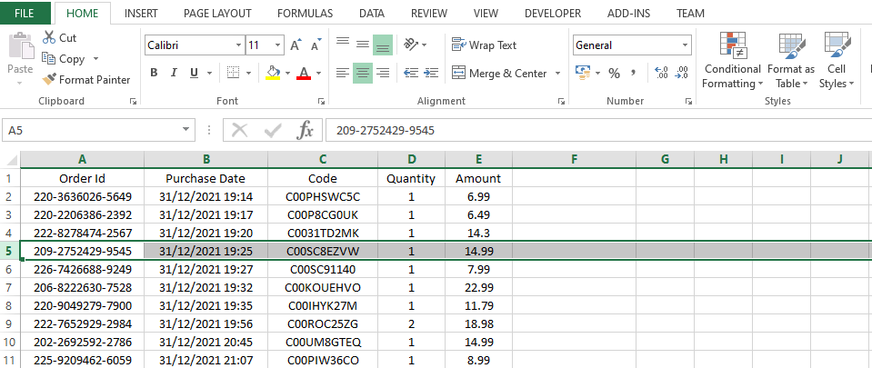
You can select an entire row with the Rows Object like this:

Rows(5).Select

Or you can use EntireRow along with the Range or Cells Objects:

Range("B5").EntireRow.Select

or

Cells(5,1).EntireRow.Select

You can also use the Range Object to refer specifically to a Row:

Range("5:5").Select

Select Single Column

Instead of the Rows Object, use the Columns Object to select columns. Here you can reference the column number 3:

Columns(3).Select

or letter “C”, surrounded by quotations:

Columns("C").Select

Instead of EntireRow, use EntireColumn along with the Range or Cells Objects to select entire columns:

Range("C5").EntireColumn.Select

or

Cells(5,3).EntireColumn.Select

You can also use the Range Object to refer specifically to a column:

Range("B:B").Select

Select Multiple Rows or Columns

Selecting multiple rows or columns works exactly the same when using EntireRow or EntireColumn:

Range("B5:D10").EntireRow.Select

or

Range("B5:B10").EntireColumn.Select

However, when you use the Rows or Columns Objects, you must enter the row numbers or column letters in quotations:

Rows("1:3").Select

or

Columns("B:C").Select

Select ActiveCell Row or Column

To select the ActiveCell Row or Column, you can use one of these lines of code:

ActiveCell.EntireRow.Select

or

ActiveCell.EntireColumn.Select

Select Rows and Columns on Other Worksheets

In order to select Rows or Columns on other worksheets, you must first select the worksheet.

Sheets("Sheet2").Select
Rows(3).Select

The same goes for when selecting rows or columns in other workbooks.

Workbooks("Book6.xlsm").Activate
Sheets("Sheet2").Select
Rows(3).Select

Note: You must Activate the desired workbook. Unlike the Sheets Object, the Workbook Object does not have a Select Method.

VBA Coding Made Easy

Stop searching for VBA code online. Learn more about AutoMacro — A VBA Code Builder that allows beginners to code procedures from scratch with minimal coding knowledge and with many time-saving features for all users!

Learn More

Is Selecting Rows and Columns Necessary?

However, it’s (almost?) never necessary to actually select Rows or Columns. You don’t need to select a Row or Column in order to interact with them. Instead, you can apply Methods or Properties directly to the Rows or Columns. The next several sections will demonstrate different Methods and Properties that can be applied.

You can use any method listed above to refer to Rows or Columns.

Methods and Properties of Rows & Columns

Delete Entire Rows or Columns

To delete rows or columns, use the Delete Method:

Rows("1:4").Delete

or:

Columns("A:D").Delete

VBA Programming | Code Generator does work for you!

Insert Rows or Columns

Use the Insert Method to insert rows or columns:

Rows("1:4").Insert

or:

Columns("A:D").Insert

Copy & Paste Entire Rows or Columns

Paste Into Existing Row or Column

When copying and pasting entire rows or columns you need to decide if you want to paste over an existing row / column or if you want to insert a new row / column to paste your data.

These first examples will copy and paste over an existing row or column:

Range("1:1").Copy Range("5:5")

or

Range("C:C").Copy Range("E:E")

Insert & Paste

These next examples will paste into a newly inserted row or column.

This will copy row 1 and insert it into row 5, shifting the existing rows down:

Range("1:1").Copy
Range("5:5").Insert

This will copy column C and insert it into column E, shifting the existing columns to the right:

Range("C:C").Copy
Range("E:E").Insert

Hide / Unhide Rows and Columns

To hide rows or columns set their Hidden Properties to True. Use False to hide the rows or columns:

'Hide Rows
Rows("2:3").EntireRow.Hidden = True

'Unhide Rows
Rows("2:3").EntireRow.Hidden = False

or

'Hide Columns
Columns("B:C").EntireColumn.Hidden = True

'Unhide Columns
Columns("B:C").EntireColumn.Hidden = False

Group / UnGroup Rows and Columns

If you want to Group rows (or columns) use code like this:

'Group Rows
Rows("3:5").Group

'Group Columns
Columns("C:D").Group

To remove the grouping use this code:

'Ungroup Rows
Rows("3:5").Ungroup

'Ungroup Columns
Columns("C:D").Ungroup

This will expand all “grouped” outline levels:

ActiveSheet.Outline.ShowLevels RowLevels:=8, ColumnLevels:=8

and this will collapse all outline levels:

ActiveSheet.Outline.ShowLevels RowLevels:=1, ColumnLevels:=1

Set Row Height or Column Width

To set the column width use this line of code:

Columns("A:E").ColumnWidth = 30

To set the row height use this line of code:

Rows("1:1").RowHeight = 30

AutoMacro | Ultimate VBA Add-in | Click for Free Trial!

Autofit Row Height / Column Width

To Autofit a column:

Columns("A:B").Autofit

To Autofit a row:

Rows("1:2").Autofit

Rows and Columns on Other Worksheets or Workbooks

To interact with rows and columns on other worksheets, you must define the Sheets Object:

Sheets("Sheet2").Rows(3).Insert

Similarly, to interact with rows and columns in other workbooks, you must also define the Workbook Object:

Workbooks("book1.xlsm").Sheets("Sheet2").Rows(3).Insert

Get Active Row or Column

To get the active row or column, you can use the Row and Column Properties of the ActiveCell Object.

MsgBox ActiveCell.Row

or

MsgBox ActiveCell.Column

This also works with the Range Object:

MsgBox Range("B3").Column

---

VBA Select

It is very common to find the .Select methods in saved macro recorder code, next to a Range object.

.Select is used to select one or more elements of Excel (as can be done by using the mouse) allowing further manipulation of them.

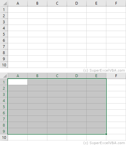
Selecting cells with the mouse:

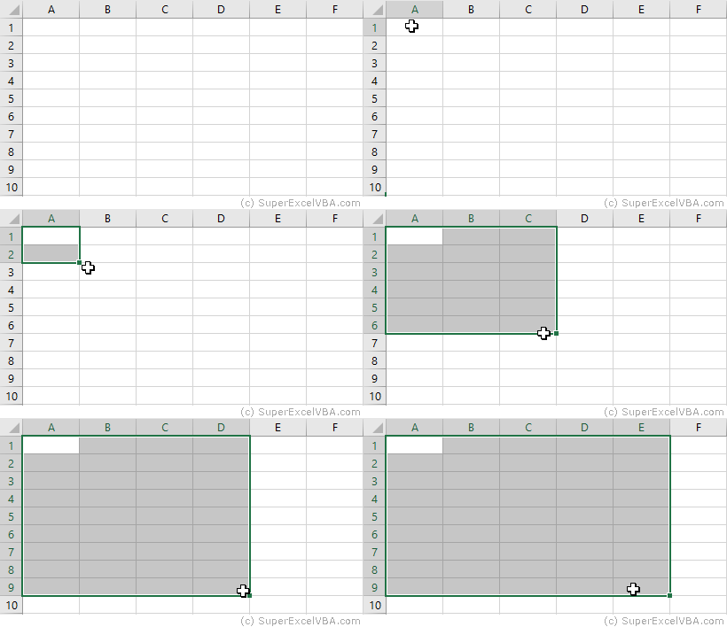
Selecting cells with VBA:

    'Range([cell1],[cell2])
    Range(Cells(1, 1), Cells(9, 5)).Select
    Range("A1", "E9").Select
    Range("A1:E9").Select

Each of the above lines select the range from «A1» to «E9».

---

VBA Select CurrentRegion

If a region is populated by data with no empty cells, an option for an automatic selection is the CurrentRegion property alongside the .Select method.

CurrentRegion.Select will select, starting from a Range, all the area populated with data.

    Range("A1").CurrentRegion.Select

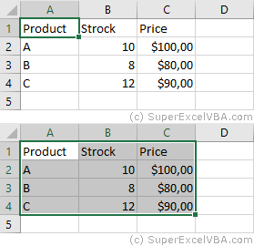
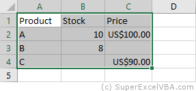
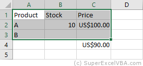
Make sure there are no gaps between values, as CurrentRegion will map the region through adjoining cells (horizontal, vertical and diagonal).

  Range("A1").CurrentRegion.Select

With all the adjacent data

Not all adjacent data

«C4» is not selected because it is not immediately adjacent to any filled cells.

---

VBA ActiveCell

The ActiveCell property brings up the active cell of the worksheet.

In the case of a selection, it is the only cell that stays white.

A worksheet has only one active cell.

    Range("B2:C4").Select
    ActiveCell.Value = "Active"

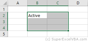
Usually the ActiveCell property is assigned to the first cell (top left) of a Range, although it can be different when the selection is made manually by the user (without macros).

The AtiveCell property can be used with other commands, such as Resize.

---

VBA Selection

After selecting the desired cells, we can use Selection to refer to it and thus make changes:

    Range("A1:D7").Select
    Selection = 7

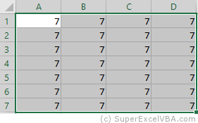
Selection also accepts methods and properties (which vary according to what was selected).

    Selection.ClearContents 'Deletes only the contents of the selection
    Selection.Interior.Color = RGB(255, 255, 0) 'Adds background color to the selection

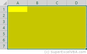
As in this case a cell range has been selected, the Selection will behave similarly to a Range. Therefore, Selection should also accept the .Interior.Color property.

RGB (Red Green Blue) is a color system used in a number of applications and languages. The input values for each color, in the example case, ranges from 0 to 255.

---

Selection FillDown

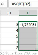
If there is a need to replicate a formula to an entire selection, you can use the .FillDown method

    Selection.FillDown

Before the FillDown

After the FillDown

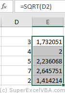
.FillDown is a method applicable to Range. Since the Selection was done in a range of cells (equivalent to a Range), the method will be accepted.

.FillDown replicates the Range/Selection formula of the first line, regardless of which ActiveCell is selected.

.FillDown can be used at intervals greater than one column (E.g. Range(«B1:C2»).FillDown will replicate the formulas of B1 and C1 to B2 and C2 respectively).

---

VBA EntireRow and EntireColumn

You can select one or multiple rows or columns with VBA.

    Range("B2").EntireRow.Select
    Range("C3:D3").EntireColumn.Select

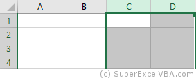
The selection will always refer to the last command executed with Select.

To insert a row use the Insert method.

    Range("A7").EntireRow.Insert
    'In this case, the content of the seventh row will be shifted downward

To delete a row use the Delete method.

    Range("A7").EntireRow.Delete
    'In this case, the content of the eighth row will be moved to the seventh

---

VBA Rows and Columns

Just like with the EntireRow and EntireColumn property, you can use Rows and Columns to select a row or column.

    Columns(5).Select
    Rows(3).Select

To hide rows:

    Range("A1:C3").Rows.Hidden = True

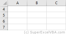
In the above example, rows 1 to 3 of the worksheet were hidden.

---

VBA Row and Column

Row and Column are properties that are often used to obtain the numerical address of the first row or first column of a selection or a specific cell.

    Range("A3:H30").Row 'Referring to the row; returns 3
    Range("B3").Column  'Referring to the column; returns 2

The results of Row and Column are often used in loops or resizing.

---

---

Consolidating Your Learning

Suggested Exercise

---

---

Need to Select Data Range in Excel

In Microsoft Excel, several operations like delete, edit, type, and other formatting can be done only if we select the range of cells we need to change. There are several ways in which we select the range of cells. In this article, we will discuss selecting a specific row or row using VBA to perform any action or format them.

Select a Row if You Know its Number

Here is the code that helps select a specific row if we know the row number. Let us select row number 15 here.

Sub row_select()

'Select the row no 15
Rows(15).Select

End Sub

Output:

Here I already have a “Simple Interest” sheet with some data. Row number 15 of the active sheet is selected.

Using the EntireRow Property

This is a property of a cell reference. We can use it in two ways, as explained below.

Using a Range Reference

We select the entire row to which a specified cell belongs.

Sub row_select()
'Select the rows that belongs to Cell G6
Range("G6").EntireRow.Select
End Sub

Output:

Since G6 belongs to row number 6, that row is selected here.

Using a Cell Reference

Sub row_select()
'Select the rows that belongs to Cell (5,3) i.e.  5th row
Cells(5, 3).EntireRow.Select
End Sub

Output:

Select 1 or More Rows:

The range object can be used to select 1 or more rows too.

The code below selects all rows from 5 to 8.

 
Sub row_select()

'Select the rows from 5 to 8
Range("5:8").EntireRow.Select

End Sub

Select All Rows That Belong to a Specific Range

Let us assume a specific range B3 to E5. Now, if we use the entire row property on this range and select, we can notice that rows 3 to 5 have been selected because the specified range belongs to these three rows.

Sub row_select()

'Select the rows that belong to a range
Range("B3:E5").EntireRow.Select

End Sub

Output:

Selection of the Row to Which the Active Cell Belongs

The code below is run after selecting cells (10, 3) or C10.

Sub row_select()

'Select the rows to which the active cell belongs
ActiveCell.EntireRow.Select

End Sub

Selecting All Rows of the Active Sheet

All rows of the active sheet (Simple interest sheet in this example) is selected.

Sub row_select()

'Select the rows of the active sheet
ActiveSheet.Rows.Select

End Sub

Output:

Select a Specific Row in a Range

In this example, the rows are not selected from the sheet. Instead, a specified range is assumed as a sheet, and the row number specified within the code is assumed as the row number within the specified range and selected. For example, we want to select the 2^nd row of the range D4 to H8. The second row of this range is row number 5 of the spreadsheet.

Sub row_select()

'Select the row within the range
Range("D4:H8").Rows(2).Select

End Sub

Output:

Now, we see that the 2^nd row of the range D4 to H8 is selected within the 5^th row of the spreadsheet.

Color Rows That Have Data in the First Column

In this example, we will consider the first 10 rows and go through the content of the first column in each row. If the cell is not null, then we will color it green.

Sub row_select()

' Loop through the first 10 rows
For i = 1 To 10

' validate if the cell is blank
If Cells(i, 1).Value <> "" Then

'select the row
Rows(i).EntireRow.Select

' colour the selected row
    With Selection.Interior
        .Pattern = xlSolid
        .PatternColorIndex = xlAutomatic
        .Color = 5296274
        .TintAndShade = 0
        .PatternTintAndShade = 0
    End With
    ' end the condition
End If
' end the loop
Next

End Sub

The rows that do not have values in column A (only until row number 10) are colored green.

Conclusion

Row selection can be used with loops and conditions in the program logic. However, unlike a manual task, most of the tasks in VBA can also be done directly without selecting cells/rows/columns/range. So, the selection operation is not always necessary.

In this lesson I will show you how to get selected rows of an Excel sheet using a macro. As developers we need to create various kinds of macros to fulfil user’s requirements. Sometimes users want to select rows manually in the excel sheet before running the macros. Then macro may need to detect the rows selected by the user before processing the data. For an example user may want to transfer selected rows to another file or sheet. Or combine data of selected rows. Those are a few examples where you need to get the selected rows. Now let’s learn how to get the selected rows using VBA.

Suppose a user has selected a one row like this.

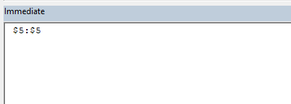
Then we can use this macro below to print the address of the row in the immediate window.

Here is the result of the above macro.

What if the user selects multiple rows like this. 

 

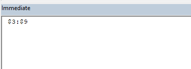
Then we will get the below result if we run the same macro.

In the above examples, the result was a string. But usually we need to get the starting row and the ending row as numbers. Then only we can use those values in the next steps. So next let’s look at how we can get the starting row and the ending row. We can create two functions to get starting and ending rows. This is the function to get the starting row.

In this function we have used two inbuilt functions. Split function and Replace function. Split function divides the string at the character “:”. For the above example, Split(SelectedRows, «:»)(0) will return $3
Then the replace function will remove the $ symbol.

And this is the function to get the ending row.

Only difference is you have to replace 0 in the split function with 1. Then the split function will split the string at character : and take the second element. Now you can use the above functions in a subroutine.

Here is the result you will get.

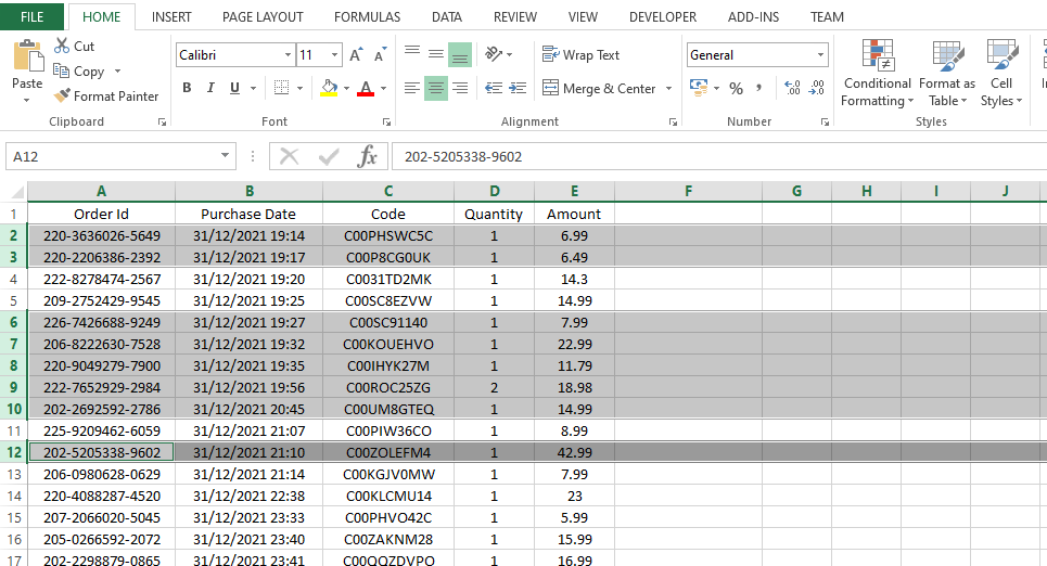
But sometimes users may select non contiguous rows like this. 

Then our first macro (GetSelectedRows) will output this result.

But then our two functions will fail to output correct results. In a next lesson I will show you how to detect a non contiguous range and output the result as a two dimensional array. 

Excel VBA Referencing Ranges — Range, Cells, Item, Rows & Columns Properties; Offset; ActiveCell; Selection; Insert

You can refer to or access a worksheet range using properties and methods of the Range object. A Range Object refers to a cell or a range of cells. It can be a row, a column or a selection of cells comprising of one or more rectangular / contiguous blocks of cells. One of the most important aspects in vba coding is referencing and using Ranges within a Worksheet. This section (divided into 2 parts) covers various properties and methods for referencing, accessing & using ranges, divided under the following chapters.

Excel VBA Referencing Ranges — Range, Cells, Item, Rows & Columns Properties; Offset; ActiveCell; Selection; Insert:

Range Property, Cells / Item / Rows / Columns Properties, Offset & Relative Referencing, Cell Address;

Activate & Select Cells; the ActiveCell & Selection;

Entire Row & Entire Column Properties, Inserting Cells/Rows/Columns using the Insert Method;

Excel VBA Refer to Ranges — Union & Intersect; Resize; Areas, CurrentRegion, UsedRange & End Properties; SpecialCells Method:

Ranges — Union & Intersect;

Resize a Range;

Referencing — Contiguous Block(s) of Cells, Range of Contiguous Data, Cells Meeting a Specified Criteria, Used Range, Cell at the End of a Block / Region, Last Used Row or Column;

---

Related Links:

Working with Objects in Excel VBA

Excel VBA Application Object, the Default Object in Excel

Excel VBA Workbook Object, working with Workbooks in Excel

Microsoft Excel VBA — Worksheets

Excel VBA Custom Classes and Objects

---

——————————————————————————————-

Contents:

Range Property, Cells / Item / Rows / Columns Properties, Offset & Relative Referencing, Cell Address

Activate & Select Cells; the ActiveCell & Selection

Entire Row & Entire Column Properties, Inserting Cells/Rows/Columns using the Insert Method

——————————————————————————————-

Range Property, Cells / Item / Rows / Columns Properties, Offset & Relative Referencing, Cell Address

A Range Object refers to a cell or a range of cells. It can be a row, a column or a selection of cells comprising of one or more rectangular / contiguous blocks of cells. A Range object is always with reference to a specific worksheet, and Excel currently does not support Range objects spread over multiple worksheets.

Range object refers to a single cell:

Dim rng As Range
Set rng = Range(«A1»)

Range object refers to a block of contiguous cells:

Dim rng As Range
Set rng = Range(«A1:C3»)

Range object refers to a row:

Dim rng As Range
Set rng = Rows(1)

Range object refers to multiple columns:

Dim rng As Range
Set rng = Columns(«A:C»)

Range object refers to 2 or more blocks of contiguous cells — using the ‘Union method’ & ‘Selection’ (these have been explained in detail later in this section).

Union method:

Dim rng1 As Range, rng2 As Range, rngUnion As Range
‘set a contiguous block of cells as the first range:
Set rng1 = Range(«A1:B2»)
‘set another contiguous block of cells as the second range:
Set rng2 = Range(«D3:E4»)
‘assign a variable (range object) to represent the union of the 2 ranges, using the Union method:
Set rngUnion = Union(rng1, rng2)
‘set interior color for the range which is the union of 2 range objects:
rngUnion.Interior.Color = vbYellow

Selection property:

‘select 2 contiguous block of cells, using the Select method:
Range(«A1:B2,D3:E4»).Select
‘perform action (set interior color of cells to yellow) on the Selection, which is a Range object:
Selection.Interior.Color = vbYellow

Range property of the Worksheet object ie. Worksheet.Range Property. Syntax: WorksheetObject.Range(Cell1, Cell2). You have an option to use only the Cell1 argument and in this case it will have to be a A1-style reference to a range which can include a range operator (colon) or the union operator (comma), or the reference to a range can be a defined name. Examples of using this type of reference are Worksheets(«Sheet1»).Range(«A1») which refers to cell A1; or Worksheets(«Sheet1»).Range(«A1:B3») which refers to the cells A1, A2, A3, B1, B2 & B3. When both the Cell1 & Cell2 arguments are used (cell1 and cell2 are Range objects), these refer to the cells at the top-left corner and the lower-right corner of the range (ie. the start and end cells of the range), and these arguments can be a single cell, an entire row or column or a single named cell. An example of using this type of reference is Worksheets(«Sheet1»).Range(Cells(1, 1), Cells(3, 2)) which refers to the cells A1, A2, A3, B1, B2 & B3. Omitting the object qualifier will default to the active sheet viz. using the code Range(«A1») will return cell A1 of the active sheet, and will be the same as using Application.Range(«A1») or ActiveSheet.Range(«A1»).

Range property of the Range object: Use the Range.Range property [Syntax: RangeObject.Range(Cell1,Cell2)] for relative referencing ie. to access a range relative to a range object. For example, Worksheets(«Sheet1»).Range(«C5:E8»).Range(«A1») will refer to Range(«C5») and Worksheets(«Sheet1»).Range(«C5:E8»).Range(«B2») will refer to Range(«D6»).

Shortcut Range Reference: As compared to using the Range property, you can also use a shorter code to refer to a range by using square brackets to enclose an A1-style reference or a name. While using square brackets, you do not type the Range word or wrap the range in quotation marks to make it a string. Using square brackets is similar to applying the Evaluate method of the Application object. The Range property or the Evaluate method use a string argument which enables you to manipulate the string with vba code, whereas using the square brackets will be inflexible in this respect. Examples: using [A1].Value = 5 is equivalent to using Range(«A1»).Value = 5; using [A1:A3,B2:B4,C3:D5].Interior.Color = vbRed is equivalent to Range(«A1:A3,B2:B4,C3:D5»).Interior.Color = vbRed; and with named ranges, [Score].Interior.Color = vbBlue is equivalent to Range(«Score»).Interior.Color = vbBlue. Using square brackets only enables reference to fixed ranges which is a significant shortcoming. Using the Range property enables you to manipulate the string argument with vba code so that you can use variables to refer to a dynamic range, as illustrated below:

Sub DynamicRangeVariable()
‘using a variable to refer a dynamic range.

Dim i As Integer

‘enters the text «Hello» in each cell from B1 to B5:
For i = 1 To 5
Range(«B» & i) = «Hello»
Next

End Sub

The Cells Property returns a Range object referring to all cells in a worksheet or a range, as it can be used with respect to an Application object, a Worksheet object or a Range object. Application.Cells Property refers to all cells in the active worksheet. You can use the code Application.Cells or omit the object qualifier (this property is a member of ‘globals’) and use the code Cells to refer to all cells of the active worksheet. The Worksheet.Cells Property (Syntax: WorksheetObject.Cells) refers to all cells of a specified worksheet. Use the code Worksheets(«Sheet1»).Cells to refer to all cells of worksheet named «Sheet1». Use the Range.Cells Property ro refer to cells in a specified range — (Syntax: RangeObject.Cells). This property can be used as Range(«A1:B5»).Cells, however using the word cells in this case is immaterial because with or without this word the code will refer to the range A1:B5. To refer to a specific cell, use the Item property of the Range object (as explained in detail below) by specifying the relative row and column positions after the Cells keyword, viz. Worksheets(«Sheet1»).Cells.Item(2, 3) refers to range C2 and Worksheets(«Sheet1»).Range(«C2»).Cells(2, 3) will refer to range E3. Because the Item property is the Range object’s default property you can omit the Item word word and use the code Worksheets(«Sheet1»).Cells(2, 3) which also refers to range C2. You may find it preferable in some cases to use Worksheets(«Sheet1»).Cells(2, 3) over Worksheets(«Sheet1»).Range(«C2») because variables for the row and column can easily be used therein.

Item property of the Range object: Use the Range.Item Property to return a range as offset to the specified range. Syntax: RangeObject.Item(RowIndex, ColumnIndex). The Item word can be omitted because Item is the Range object’s default property. It is necessary to specify the RowIndex argument while ColumnIndex is optional. RowIndex is the index number of the cell, starting with 1 and increasing from left to right and then down. Worksheets(«Sheet1»).Cells.Item(1) or Worksheets(«Sheet1»).Cells(1) refers to range A1 (the top-left cell in the worksheet), Worksheets(«Sheet1»).Cells(2) refers to range B1 (cell next to the right of the top-left cell). While using a single-parameter reference of the Item property (ie. RowIndex), if index exceeds the number of columns in the specified range, the reference will wrap to successive rows within the range columns. Omitting the object qualifier will default to active sheet. Cells(16385) refers to range A2 of the active sheet in Excel 2007 which has 16384 columns, and Cells(16386) refers to range B2, and so on. Also note that RowIndex and ColumnIndex are offsets and relative to the specified Range (ie. relative to the top-left corner of the specified range). Both Range(«B3»).Item(1) and Range(«B3:D6»).Item(1) refer to range B3. The following refer to range D4, the sixth cell in the range: Range(«B3:D6»).Item(6) or Range(«B3:D6»).Cells(6) or Range(«B3:D6»)(6). ColumnIndex refers to the column number of the cell, can be a number starting with 1 or can be a string starting with the letter «A». Worksheets(«Sheet1»).Cells(2, 3) and Worksheets(«Sheet1»).Cells(2, «C») both refer to range C2 wherein the RowIndex is 2 and ColumnIndex is 3 (column C). Range(«C2»).Cells(2, 3) refers to range E3 in the active sheet, and Range(«C2»).Cells(4, 5) refers to range G5 in the active sheet. Using Range(«C2»).Item(2, 3) and Range(«C2»).Item(4, 5) has the same effect and will refer to range E3 & range G5 respectively. Using Range(«C2:D3»).Cells(2, 3) and Range(«C2:D3»).Cells(4, 5) will also refer to range E3 & range G5 respectively. Omitting the Item or Cells word — Range(«C2:D3»)(2, 3) and Range(«C2:D3»)(4, 5) also refers to range E3 & range G5 respectively. It is apparant here that you can refer to and return cells outside the original specified range, using the Item property.

Columns property of the Worksheet object: Use the Worksheet.Columns Property (Syntax: WorksheetObject.Columns) to refer to all columns in a worksheet  which are returned as a Range object. Example: Worksheets(«Sheet1»).Columns will return all columns of the worksheet; Worksheets(«Sheet1»).Columns(1) returns the first column (column A) in the worksheet; Worksheets(«Sheet1»).Columns(«A») returns the first column (column A); Worksheets(«Sheet1»).Columns(«A:C») returns the columns A, B & C; and so on. Omitting the object qualifier will default to the active sheet viz. using the code Columns(1) will return the first column of the active sheet, and will be the same as using Application.Columns(1).

Columns property of the Range object: Use the Range.Columns Property (Syntax: RangeObject.Columns) to refer to columns in a specified range. Example1: color cells from all columns of the specified range ie. B2 to D4: Worksheets(«Sheet1»).Range(«B2:D4»).Columns.Interior.Color = vbYellow. Example2: color cells from first column of the range only ie. B2 to B4: Worksheets(«Sheet1»).Range(«B2:D4»).Columns(1).Interior.Color = vbGreen. If the specified range object contains multiple areas, the columns from the first area only will be returned by this property (Areas property has been explained in detail later in this section). Take the example of 2 areas in the specified range, first area being «B2:D4» and the second area being «F3:G6» — the following code will color cells from first column of the first area only ie. cells B2 to B4: Worksheets(«Sheet1»).Range(«B2:D4, F3:G6»).Columns(1).Interior.Color = vbRed. Omitting the object qualifier will default to active sheet — following will apply color to column A of the ActiveSheet: Columns(1).Interior.Color = vbRed.

Use the Worksheet.Rows Property (Syntax: WorksheetObject.Rows) to refer to all rows in a worksheet  which are returned as a Range object. Example: Worksheets(«Sheet1»).Rows will return all rows of the worksheet; Worksheets(«Sheet1»).Rows(1) returns the first row (row one) in the worksheet; Worksheets(«Sheet1»).Rows(3) returns the third row (row three) in the worksheet; Worksheets(«Sheet1»).Rows(«1:3») returns the first 3 rows; and so on. Omitting the object qualifier will default to the active sheet viz. using the code Rows(1) will return the first row of the active sheet, and will be the same as using Application.Rows(1).

Use the Range.Rows Property (Syntax: RangeObject.Rows) to refer to rows in a specified range. Example1: color cells from all rows of the specified range ie. B2 to D4: Worksheets(«Sheet1»).Range(«B2:D4»).Rows.Interior.Color = vbYellow. Example2: color cells from first row of the range only ie. B2 to D2: Worksheets(«Sheet1»).Range(«B2:D4»).Rows(1).Interior.Color = vbGreen. If the specified range object contains multiple areas, the rows from the first area only will be returned by this property (Areas property has been explained in detail later in this section). Take the example of 2 areas in the specified range, first area being «B2:D4» and the second area being «F3:G6» — the following code will color cells from first row of the first area only ie. cells B2 to D2: Worksheets(«Sheet1»).Range(«B2:D4, F3:G6»).Rows(1).Interior.Color = vbRed. Omitting the object qualifier will default to active sheet — following will apply color to row one of the ActiveSheet: Rows(1).Interior.Color = vbRed.

To refer to a range as offset from a specified range, use the Range.Offset Property. Syntax: RangeObject.Offset(RowOffset, ColumnOffset). Both arguments are optional to specify. The RowOffset argument specifies the number of rows by which the specified range is offset — negative values indicating upward offset and positive values indicating downward offset, with default value being 0. The ColumnOffset argument specifies the number of columns by which the specified range is offset — negative values indicating left offset and positive values indicating right offset, with default value being 0. Examples: Range(«C5»).Offset(1, 2) offsets 1 row & 2 columns and refers to Range E6, Range(«C5:D7»).Offset(1, -2) offsets 1 row downward & 2 columns to the left and refers to Range (A6:B8).

Accessing a worksheet range, with vba code:-

Referencing a single cell:

Enter the value 10 in the cell A1 of the worksheet named «Sheet1» (omitting to mention a property with the Range object will assume the Value property, as shown below):

Worksheets(«Sheet1»).Range(«A1»).Value = 10

Worksheets(«Sheet1»).Range(«A1») = 10

Enter the value of 10 in range C2 of the active worksheet — using Cells(row, column) where row is the row index and column is the column index:

ActiveSheet.Cells(2, 3).Value = 10

Referencing a range of cells:

Enter the value 10 in the cells A1, A2, A3, B1, B2 & B3 (wherein the cells refer to the upper-left corner & lower-right corner of the range) of the active sheet:

ActiveSheet.Range(«A1:B3»).Value = 10

ActiveSheet.Range(«A1», «B3»).Value = 10

ActiveSheet.Range(Cells(1, 1), Cells(3, 2)) = 10

Enter the value 10 in the cells A1 & B3 of worksheet named «Sheet1»:

Worksheets(«Sheet1»).Range(«A1,B3»).Value = 10

Set the background color (red) for cells B2, B3, C2, C3, D2, D3 & H7 of worksheet named «Sheet3»:

ActiveWorkbook.Worksheets(«Sheet3»).

Range(«B2:D3,H7»).Interior.Color = vbRed

Enter the value 10 in the Named Range «Score» of the active worksheet, viz. you can name the Range(«B2:B3») as «Score» to insert 10 in the cells B2 & B3:

Range(«Score»).Value = 10

ActiveSheet.Range(«Score»).Value = 10

Select all the cells of the active worksheet:

ActiveSheet.Cells.Select

Cells.Select

Set the font to «Times New Roman» & the font size to 11, for all the cells of the active worksheet in the active workbook:

ActiveWorkbook.ActiveSheet.Cells.Font.Name = «Times New Roman»

ActiveSheet.Cells.Font.Size = 11

Cells.Font.Size = 11

Referencing Row(s) or Column(s):

Select all the Rows of active worksheet:

ActiveSheet.Rows.Select

Enter the value 10 in the Row number 2 (ie. every cell in second row), of worksheet named «Sheet1»:

Worksheets(«Sheet1»).Rows(2).Value = 10

Select all the Columns of the active worksheet:

ActiveSheet.Columns.Select

Columns.Select

Enter the value 10 in the Column number 3 (ie. every cell in column C), of the active worksheet:

ActiveSheet.Columns(3).Value = 10

Columns(«C»).Value = 10

Enter the value 10 in Column numbers 1, 2 & 3 (ie. every cell in columns A to C), of worksheet named «Sheet1»:

Worksheets(«Sheet1»).Columns(«A:C»).Value = 10

Relative Referencing:

Inserts the value 10 in Range C5 — reference starts from upper-left corner of the defined Range:

Range(«C5:E8»).Range(«A1») = 10

Inserts the value 10 in Range D6 — reference starts from upper-left corner of the defined Range:

Range(«C5:E8»).Range(«B2») = 10

Inserts the value 10 in Range E6 — offsets 1 row & 2 columns, using the Offset property:

Range(«C5»).Offset(1, 2) = 10

Inserts the value 10 in Range(«F7:H10») — offsets 2 rows & 3 columns, using the Offset property:

Range(«C5:E8»).Offset(2, 3) = 10

Example 1 — Using Range, Cells, Columns & Rows property — refer Image 1:

Sub CellsColumnsRowsProperty()
‘using Range, Cells, Columns & Rows property — refer Image 1:

‘enter numbers starting from 1 in each row, for a 5 row & 5 column range (A1:E5):

For r = 1 To 5

n = 1

For c = 1 To 5

Cells(r, c).Value = n

n = n + 1

Next c

Next r

‘set range to A1:E5, wherein the numbers have been entered as above:
Set rng = Range(Cells(1, 1), Cells(5, 5))

‘set background color of each even number column to yellow and of each odd number column to green:

For i = 1 To 5

If i Mod 2 = 0 Then

rng.Columns(i).Interior.Color = vbYellow
Else

rng.Columns(i).Interior.Color = vbGreen

End If

Next i

‘set font color to red and set font to bold for of even number rows:

For j = 1 To 5

If j Mod 2 = 0 Then

rng.Rows(j).Font.Bold = True

rng.Rows(j).Font.Color = vbRed

End If

Next j

‘set font for all cells of the range to italics:
rng.Cells.Font.Italic = True

End Sub

To return the number of the first row in a range, use the Range.Row Property. If the specified range contains multiple areas, this property will return the number of the first row in the first area (Areas property has been explained in detail later in this section). Syntax: RangeObject.Row. To return the number of the first column in a range, use the Range.Column Property. If the specified range contains multiple areas, this property will return the number of the first column in the first area. Syntax: RangeObject.Column.

Examples:

Get the number of the first row in the specified range — returns 4:

MsgBox ActiveSheet.Range(«B4»).Row

MsgBox Worksheets(«Sheet1»).Range(«B4:D7»).Row

Get the number of the first column in the specified range — returns 2:

MsgBox ActiveSheet.Range(«B4:D7»).Column

Get the number of the last row in the specified range — returns 7:

Explanation: Range(«B4:D7»).Rows.Count returns 4 (the number of rows in the range). Range(«B4:D7»).Rows(Range(«B4:D7»).Rows.Count) or Range(«B4:D7»).Rows(4), returns the last row in the specified range.

MsgBox Range(«B4:D7»).Rows(Range(«B4:D7»).

Rows.Count).Row

Example 2: Using Row Property, Column Property & Rows Property, determine row number & column number, and alternate rows — refer Image 2.

Sub RowColumnProperty()
‘Using Row Property, Column Property & Rows Property, determine row number & column number, and alternate rows — refer Image 2.

‘enter its row number & column number within each cell in the specified range:

For Each cell In rng

cell.Value = cell.Row & «,» & cell.Column

Next

‘set background color of each alternate row of the specified range:

For i = 1 To rng.Rows.count

If i Mod 2 = 1 Then

rng.Rows(i).Interior.Color = vbGreen

Else

rng.Rows(i).Interior.Color = vbYellow

End If

Next

End Sub

Also refer to Example 23, of using the End & Row properties to determine the last used row or column with data.

You can get a Range reference in vba language by using the Range.Address Property, which returns the address of a Range as a string value. This property is read-only.

Examples of using the Address Property:

Returns $B$2:

MsgBox Range(«B2»).Address

Returns $B$2,$C$3:

MsgBox Range(«B2,C3»).Address

Returns $A$1:$B$2,$C$3,$D$4:

Dim strRng As String
Range(«A1:B2,C3,D4»).Select
strRng = Selection.Address
MsgBox strRng

Returns $B2:

MsgBox Range(«B2»).Address(RowAbsolute:=False)

Returns B$2:

MsgBox Range(«B2»).Address(ColumnAbsolute:=False)

Returns R2C2:

MsgBox Range(«B2»).Address(ReferenceStyle:=xlR1C1)

Includes the worksheet (active sheet — «Sheet1») & workbook («Book1.xlsm») name, and returns [Book1.xlsm]Sheet1!$B$2:

MsgBox Range(«B2»).Address(External:=True)

Returns R[1]C[-1] — Range(«B2») is 1 row and -1 columns relative to Range(«C1»):

MsgBox Range(«B2»).Address(RowAbsolute:=False, ColumnAbsolute:=False, ReferenceStyle:=xlR1C1, RelativeTo:=Range(«C1»))

Returns RC[-2] — Range(«A1») is 0 row and -2 columns relative to Range(«C1»):

MsgBox Cells(1, 1).Address(RowAbsolute:=False, ColumnAbsolute:=False, ReferenceStyle:=xlR1C1, RelativeTo:=Range(«C1»))

Activate & Select Cells; the ActiveCell & Selection

The Select method (of the Range object) is used to select a cell or a range of cells in a worksheet — Syntax: RangeObject.Select. Ensure that the worksheet wherein the Select method is applied to select cells, is the active sheet. The ActiveCell Property (of the Application object) returns a single active cell (Range object) in the active worksheet. Remember that the ActiveCell property will not work if the active sheet is not a worksheet. When a cell(s) is selected in the active window, the Selection property (of the Application object) returns a Range object representing all cells which are currently selected in the active worksheet. A Selection may consist of a single cell or a range of multiple cells, but there will only be one active cell within it, which is returned by using the ActiveCell property. When only a single cell is selected, the ActiveCell property returns this cell. On selecting multiple cells using the Select method, the first referenced cell becomes the active cell, and thereafter you can change the active cell using the Activate method. Both the ActiveCell Property & the Selection property are read-only, and not specifying the Application object qualifier viz. Application.ActiveCell or ActiveCell, Application.Selection or Selection, will have the same effect. To activate a single cell within the current selection, use the Activate Method (of the Range object) — Syntax: RangeObject.Activate, and this activated cell is returned by using the ActiveCell property.

We have discussed above that a Selection may consist of a single cell or a range of multiple cells, whereas there can be only one active cell within the Selection. When you activate a cell outside the current selection, the activated cell becomes the only selected cell. You can also use the Activate method to specify a range of multiple cells, but in effect only a single cell will be activated, and this activated cell will be the top-left corner cell of the range specified in the method. If this top-left cell lies within the selection, the current selection will not change, but if this top-left cell lies outside the selection, then the specified range in the Activate method becomes the new selection.

See below codes which illustrate the concepts of ActiveCell and Selection.

Selection containing a range of cells, and the active cell:

‘selects range C1:F5:
Range(«C1:F5»).Select
‘returns C1, the first referenced cell, as the active cell:
MsgBox ActiveCell.Address

Selection containing a range of cells, and the active cell:

‘selects range C1:F5:
Range(«F5:C1»).Select
‘returns C1, the first referenced cell, as the active cell:
MsgBox ActiveCell.Address

Selection containing a range of cells, and the active cell:

‘selects range C1:F5:
Range(«C5:F1»).Select
‘returns C1, the first referenced cell, as the active cell:
MsgBox ActiveCell.Address

Activate a cell within the current selection:

‘selects range B6:F10:
Range(«B6:F10»).Select
‘returns B6, the first referenced cell, as the active cell:
MsgBox ActiveCell.Address

‘selection remains same — range B6:F10, but the active cell is now C8:
Range(«C8»).Activate
MsgBox ActiveCell.Address

Activate a cell outside the current selection:

‘selects range B6:F10:
Range(«B6:F10»).Select
‘returns B6, the first referenced cell, as the active cell:
MsgBox ActiveCell.Address

‘both the selection and the active cell is now A2:
Range(«A2»).Activate
MsgBox ActiveCell.Address

Select a cell within the current selection:

Activate a range of cells whose top-left cell is within the current selection:

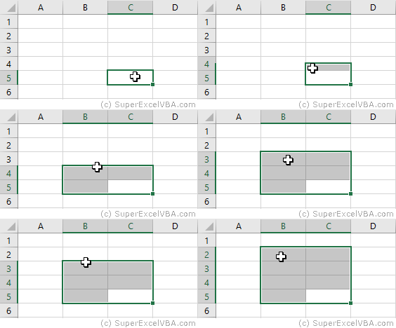
‘selects range B6:F10 — refer Image 3a:
Range(«B6:F10»).Select
‘returns B6, the first referenced cell, as the active cell:
MsgBox ActiveCell.Address

‘selection remains same — range B6:F10, but the active cell is now C8 — refer Image 3b:
Range(«C8:G12»).Activate
MsgBox ActiveCell.Address

Activate a range of cells whose top-left cell is outside the current selection:

‘selects range B6:F10 — refer Image 3a:
Range(«B6:F10»).Select
‘returns B6, the first referenced cell, as the active cell:
MsgBox ActiveCell.Address

‘selection range changes to range B1:F8, and the active cell is now B1 — refer Image 3c:
Range(«B1:F8»).Activate
MsgBox ActiveCell.Address

Using the Application.Selection Property returns the selected object wherein the selection determines the returned object type. Where the selection is a range of cells, this property returns a Range object, and this Selection — which is a Range object — can comprise of a single cell, or multiple cells or multiple non-contiguous ranges. And as mentioned above, the Select method (of the Range object) is used to select a cell or a range of cells in a worksheet. Therefore, after selecting a range, you can perform actions on the selection of cells by using the Selection object. See below illustration. 

Sub SelectionObject()

‘select cells in the active sheet using the Range.Select method:

Range(«A1:B3,D6»).Select

‘perform action (set interior color of cells to red) on the Selection, which is a Range object:

Selection.Interior.Color = vbRed

End Sub

Entire Row & Entire Column Properties, Inserting Cells/Rows/Columns using the Insert Method

Use the Range.EntireRow Property to return an entire row or rows within which the specific range is contained. Using this property returns a Range object referring to the entire row(s). Syntax: RangeObject.EntireRow. Use the Range.EntireColumn Property to return an entire column or columns within which the specific range is contained. Using this property returns a Range object referring to the entire column(s). Syntax: RangeObject.EntireColumn.

Examples of using the EntireRow & EntireColumn Properties

Selects row no. 2:

Range(«A2»).EntireRow.Select

Selects row nos. 2, 3 & 4:

Range(«A2:C4»).EntireRow.Select

Enters value 3 in range A3 ie. in the first cell of row no. 3:

Cells(3, 4).EntireRow.Cells(1, 1).Value = 3

Selects column A:

Range(«A2»).EntireColumn.Select

Selects columns A to C:

Range(«A2:C4»).EntireColumn.Select

Enters value 4 in range D1 ie. in the first cell of column no. 4:

Cells(3, 4).EntireColumn.Cells(1, 1).Value = 4

Use the Range.Insert Method to insert a cell or a range of cells in a worksheet. Syntax: RangeObject.Insert(Shift, CopyOrigin). Both arguments are optional to specify. When you insert cell(s) the other cells are shifted to make way, and you can set a value for the Shift argument to determine the direction in which the other cells are shifted — specifying xlShiftDown (value -4121) will shift the cells down, and xlShiftToRight (value -4161) shifts the cells to the right. Omitting this argument will decide the shift direction based on the shape of the range. Specifying xlFormatFromLeftOrAbove (value 0) for the CopyOrigin argument will copy the format for inserted cell(s) from the above cells or cells to the left, and specifying xlFormatFromRightOrBelow (value 1) will copy format from the below cells or cells to the right.

Illustrating Range.Insert Method — for start data refer Image 4a:

Shifts cells down and copies formatting of inserted cell from above cell — refer image 4b:

Range(«B2»).Insert

Shifts cells to the right and copies formatting of inserted cells from cells to the left — refer image 4c:

Range(«B2:C4»).Insert

Shifts cells down and copies formatting of inserted cells from above cells — refer image 4d:

Range(«B2:D3»).Insert

Shifts cells down and copies formatting of inserted cells from below cells — refer image 4e:

Range(«B2:D3»).Insert CopyOrigin:=xlFormatFromRightOrBelow

Shifts cells to the right and copies formatting of inserted cells from cells to the left — refer image 4f:

Range(«B2:D3»).Insert shift:=xlShiftToRight

Shifts cells to the right and copies formatting of inserted cells from cells to the right — refer image 4g:

Range(«B2:D3»).Insert shift:=xlShiftToRight, CopyOrigin:=xlFormatFromRightOrBelow

Inserts 2 rows — row no 2 & 3 — and copies formatting of inserted rows from above cells — refer image 4h:

Range(«B2:D3»).EntireRow.Insert

Below are some illustrations of inserting entire row(s) or column(s) dynamically in a worksheet.

Example 3: Insert row or column — specify the row / column to insert.

Sub InsertRowColumn()
‘Insert row or column — specify the row / column to insert:

ws.Range(«C3»).EntireColumn.Offset(0, 1).Insert

End Sub

Example 4: Insert row(s) after a specified value is found.

Sub InsertRow1()
‘insert row(s) after a specified value is found:

‘exit procedure if value not found:

If Not rngFind Is Nothing Then

lFindRow = rngFind.Row

MsgBox lFindRow

Else

MsgBox «Value not found!»

Exit Sub

End If

ws.Cells(lFindRow + 2, 1).EntireRow.Resize(3).Insert

End Sub

Example 5: Insert a row, n rows above the last used row.

Sub InsertRow2()
‘insert a row, n rows above the last used row

‘check if there are enough rows before the last used row, else you will get an error:

If lRowsC >= n Then

‘insert a row, n rows above the last used row — if last used row is no 5 before insertion, then insert as row no 1 and the last used row will become no 6 (similarly, if last used row is 27, then insert as row no 23) :

ws.Rows(lRowsC).Offset(-n + 1, 0).EntireRow.Insert

Else

MsgBox «Not enough rows before the last used row!»

End If

End Sub

Example 6: Insert a row each time the searched value is found in a range.

For live code of this example, click to download excel file.

Sub InsertRow3()
‘search value in a range and insert a row each time the value is found.
‘you can set the search range with the variable rngSearch in below code — the code will look within this range to find the value below which row is to be inserted.

If rngFind Is Nothing Then

MsgBox «Value not found!»

Exit Sub

Else

‘save cell address of first value found:

strAddress = rngFind.Address

Do

‘find next occurrence of value:

Set rngFind = rngSearch.FindNext(After:=rngFind)

‘insert row below when value is found (if value is found twice in a row, then 2 rows will be inserted):

rngFind.Offset(1).EntireRow.Insert

‘loop till reaching the first value found range:

Loop While rngFind.Address <> strAddress

End If

End Sub

Example 7: Insert rows (user-defined number) within consecutive values found in a column — refer Images 5a & 5b.

For live code of this example, click to download excel file.

Sub InsertRow4()
‘insert rows (user-defined number) wherever 2 consecutive values are found in a column.
‘set column number in which 2 consecutive values are checked to insert rows, using the variable lCellColumn in below code.
‘set row number from where to start searching consecutive values, using the variable lCellRow in below code.
‘refer Image 5a which shows raw data, and Image 5b after this procedure is executed — a single row (lRowsInsert value entered as 1 in input box) is inserted where consecutive values appear in column 1:

If lRowsInsert < 1 Then

MsgBox «Error — please enter a value equal to or greater than 1»

Exit Sub

End If

‘loop till the row number equals the last used row (ie. loop right till the end value in the column):

Do While lCellRow < lLastUsedRow

Set rng = Cells(lCellRow, lCellColumn)

‘in case of 2 consecutive values:

If rng <> «» And rng.Offset(1, 0) <> «» Then

‘enter the user-defined number of rows:

Range(rng.Offset(1, 0), rng.Offset(lRowsInsert, 0)).EntireRow.Insert

lCellRow = lCellRow + lRowsInsert + 1

‘determine the last used row — it is dynamic and changes on insertion of rows:

lLastUsedRow = Cells(Rows.count, lCellColumn).End(xlUp).Row

‘alternate method to determine the last used row, when number of rows inserted is fixed — this is faster than using End(xlUp):

‘lLastUsedRow = lLastUsedRow + lRowsInsert + 1

‘MsgBox lLastUsedRow

Else

lCellRow = lCellRow + 1

End If

Loop

End Sub