Excel vba select a range of sheets

Download Article

This wikiHow teaches you how to start using Visual Basic procedures to select data in Microsoft Excel. As long as you’re familiar with basic VB scripting and using more advanced features of Excel, you’ll find the selection process pretty straight-forward.

1
Select one cell on the current worksheet. Let’s say you want to select cell E6 with Visual Basic. You can do this with either of the following options:^[1]
```
ActiveSheet.Cells(6, 5).Select
```
```
ActiveSheet.Range("E6").Select
```
2
Select one cell on a different worksheet in the same workbook. Let’s say our example cell, E6, is on a sheet called Sheet2. You can use either of the following options to select it:
```
Application.Goto ActiveWorkbook.Sheets("Sheet2").Cells(6, 5)
```
```
Application.Goto (ActiveWorkbook.Sheets("Sheet2").Range("E6"))
```
Advertisement
3
Select one cell on a worksheet in a different workbook. Let’s say you want to select a cell from Sheet1 in a workbook called BOOK2.XLS. Either of these two options should do the trick:
```
Application.Goto Workbooks("BOOK2.XLS").Sheets("Sheet1").Cells(2,1)
```
```
Application.Goto Workbooks("BOOK2.XLS").Sheets("Sheet1").Range("A2")
```
4
Select a cell relative to another cell. You can use VB to select a cell based on its location relative to the active (or a different) cell. Just be sure the cell exists to avoid errors. Here’s how to use :
- Select the cell three rows below and four columns to the left of the active cell:
```
ActiveCell.Offset(3, -4).Select
```
- Select the cell five rows below and four columns to the right of cell C7:
```
ActiveSheet.Cells(7, 3).Offset(5, 4).Select
```

1
Select a range of cells on the active worksheet. If you wanted to select cells C1:D6 on the current sheet, you can enter any of the following three examples:
```
ActiveSheet.Range(Cells(1, 3), Cells(6, 4)).Select
```
```
ActiveSheet.Range("C1:D6").Select
```
```
ActiveSheet.Range("C1", "D6").Select
```
2
Select a range from another worksheet in the same workbook. You could use either of these examples to select cells C3:E11 on a sheet called Sheet3:
```
Application.Goto ActiveWorkbook.Sheets("Sheet3").Range("C3:E11")
```
```
Application.Goto ActiveWorkbook.Sheets("Sheet3").Range("C3", "E11")
```
3
Select a range of cells from a worksheet in a different workbook. Both of these examples would select cells E12:F12 on Sheet1 of a workbook called BOOK2.XLS:
```
Application.Goto Workbooks("BOOK2.XLS").Sheets("Sheet1").Range("E12:F12")
```
```
Application.Goto Workbooks("BOOK2.XLS").Sheets("Sheet1").Range("E12", "F12")
```
4
Select a named range. If you’ve assigned a name to a range of cells, you’d use the same syntax as steps 4-6, but you’d replace the range address (e.g., «E12», «F12») with the range’s name (e.g., «Sales»). Here are some examples:
- On the active sheet:
```
ActiveSheet.Range("Sales").Select
```
- Different sheet of same workbook:
```
Application.Goto ActiveWorkbook.Sheets("Sheet3").Range("Sales")
```
- Different workbook:
```
Application.Goto Workbooks("BOOK2.XLS").Sheets("Sheet1").Range("Sales")
```
5
Select a range relative to a named range. The syntax varies depending on the named range’s location and whether you want to adjust the size of the new range.
- If the range you want to select is the same size as one called Test5 but is shifted four rows down and three columns to the right, you’d use:
```
ActiveSheet.Range("Test5").Offset(4, 3).Select
```
- If the range is on Sheet3 of the same workbook, activate that worksheet first, and then select the range like this:
```
Sheets("Sheet3").Activate ActiveSheet.Range("Test").Offset(4, 3).Select
```
6
Select a range and resize the selection. You can increase the size of a selected range if you need to. If you wanted to select a range called Database’ and then increase its size by 5 rows, you’d use this syntax:
```
Range("Database").Select Selection.Resize(Selection.Rows.Count + 5, _Selection.Columns.Count).Select
```
7
Select the union of two named ranges. If you have two overlapping named ranges, you can use VB to select the cells in that overlapping area (called the «union»). The limitation is that you can only do this on the active sheet. Let’s say you want to select the union of a range called Great and one called Terrible:
- ```
Application.Union(Range("Great"), Range("Terrible")).Select
```
- If you want to select the intersection of two named ranges instead of the overlapping area, just replace Application.Union with Application.Intersect.

1

Use this example data for the examples in this method. This chart full of example data, courtesy of Microsoft, will help you visualize how the examples behave:^[2]

A1: Name B1: Sales C1: Quantity

A2: a B2: $10 C2: 5

A3: b B3: C3: 10

A4: c B4: $10 C4: 5

A5: B5: C5:

A6: Total B6: $20 C6: 20
2
Select the last cell at the bottom of a contiguous column. The following example will select cell A4:
```
ActiveSheet.Range("A1").End(xlDown).Select
```
3
Select the first blank cell below a column of contiguous cells. The following example will select A5 based on the chart above:
```
ActiveSheet.Range("A1").End(xlDown).Offset(1,0).Select
```
4
Select a range of continuous cells in a column. Both of the following examples will select the range A1:A4:
```
ActiveSheet.Range("A1", ActiveSheet.Range("a1").End(xlDown)).Select
```
```
ActiveSheet.Range("A1:" & ActiveSheet.Range("A1"). End(xlDown).Address).Select
```
5
Select a whole range of non-contiguous cells in a column. Using the data table at the top of this method, both of the following examples will select A1:A6:
```
ActiveSheet.Range("A1",ActiveSheet.Range("A65536").End(xlUp)).Select
```
```
ActiveSheet.Range("A1",ActiveSheet.Range("A65536").End(xlUp)).Select
```

Ask a Question

200 characters left

Include your email address to get a message when this question is answered.

Submit

Video

The «ActiveSheet» and «ActiveWorkbook» properties can usually be omitted if the active sheet and/or workbook(s) are implied.

Thanks for submitting a tip for review!

About This Article

Article SummaryX

1. Use ActiveSheet.Range(«E6»).Select to select E6 on the active sheet.
2. Use Application.Goto (ActiveWorkbook.Sheets(«Sheet2»).Range(«E6»)) to select E6 on Sheet2.
3. Add Workbooks(«BOOK2.XLS») to the last step to specify that the sheet is in BOOK2.XLS.

Did this summary help you?

Thanks to all authors for creating a page that has been read 167,714 times.

Is this article up to date?

Источник

Хитрости »

27 Июль 2013 306891 просмотров

Полагаю не совру когда скажу, что все кто программирует в VBA очень часто в своих кодах общаются к ячейкам листов. Ведь это чуть ли не основное предназначение VBA в Excel. В принципе ничего сложного в этом нет. Например, чтобы записать в ячейку A1 слово Привет необходимо выполнить код:

Range("A1").Value = "Привет"

Тоже самое можно сделать сразу для нескольких ячеек:

Range("A1:C10").Value = "Привет"

Если необходимо обратиться к именованному диапазону:

Range("Диапазон1").Select

Диапазон1 — это имя диапазона/ячейки, к которому надо обратиться в коде. Указывается в кавычках, как и адреса ячеек.
Но в VBA есть и альтернативный метод записи значений в ячейке — через объект Cells:

Cells(1, 1).Value = "Привет"

Синтаксис объекта Range:
Range(Cell1, Cell2)

Cell1 — первая ячейка диапазона. Может быть ссылкой на ячейку или диапазон ячеек, текстовым представлением адреса или имени диапазона/ячейки. Допускается указание несвязанных диапазонов(A1,B10), пересечений(A1 B10).
Cell2 — последняя ячейка диапазона. Необязательна к указанию. Допускается указание ссылки на ячейку, столбец или строку.

Синтаксис объекта Cells:
Cells(Rowindex, Columnindex)

Rowindex — номер строки
Columnindex — номер столбца

Исходя из этого несложно предположить, что к диапазону можно обратиться, используя Cells и Range:

'выделяем диапазон "A1:B10" на активном листе
Range(Cells(1,1), Cells(10,2)).Select

и для чего? Ведь можно гораздо короче:

Иногда обращение посредством Cells куда удобнее. Например для цикла по столбцам(да еще и с шагом 3) совершенно неудобно было бы использовать буквенное обозначение столбцов.
Объект Cells так же можно использовать для указания ячеек внутри непосредственно указанного диапазона. Например, Вам необходимо выделить ячейку в 3 строке и 2 столбце диапазона «D5:F56». Можно пройтись по листу и посмотреть, отсчитать нужное количество строк и столбцов и понять, что это будет «E7». А можно сделать проще:

Range("D5:F56").Cells(3, 2).Select

Согласитесь, это гораздо удобнее, чем отсчитывать каждый раз. Особенно, если придется оперировать смещением не на 2-3 ячейки, а на 20 и более. Конечно, можно было бы применить Offset. Но данное свойство именно смещает диапазон на указанное количество строк и столбцов и придется уменьшать на 1 смещение каждого параметра для получения нужной ячейки. Да и смещает на указанное количество строк и столбцов весь диапазон, а не одну ячейку. Это, конечно, тоже не проблема — можно вдобавок к этому использовать метод Resize — но запись получится несколько длиннее и менее наглядной:

Range("D5:F56").Offset(2, 1).Resize(1, 1).Select

И неплохо бы теперь понять, как значение диапазона присвоить переменной. Для начала переменная должна быть объявлена с типом Range. А т.к. Range относится к глобальному типу Object, то присвоение значения такой переменной должно быть обязательно с применением оператора Set:

Dim rR as Range
Set rR = Range("D5")

если оператор Set не применять, то в лучшем случае получите ошибку, а в худшем(он возможен, если переменной rR не назначать тип) переменной будет назначено значение Null или значение ячейки по умолчанию. Почему это хуже? Потому что в таком случае код продолжит выполняться, но логика кода будет неверной, т.к. эта самая переменная будет содержать значение неверного типа и применение её в коде в дальнейшем все равно приведет к ошибке. Только ошибку эту отловить будет уже сложнее.
Использовать же такую переменную в дальнейшем можно так же, как и прямое обращение к диапазону:

Вроде бы на этом можно было завершить, но…Это как раз только начало. То, что я написал выше знает практически каждый, кто пишет в VBA. Основной же целью этой статьи было пояснить некоторые нюансы обращения к диапазонам. Итак, поехали.

Обычно макрорекордер при обращении к диапазону(да и любым другим объектам) сначала его выделяет, а потом уже изменяет свойство или вызывает некий метод:

'так выглядит запись слова Test в ячейку А1
Range("A1").Select
Selection.Value = "Test"

Но как правило выделение — действие лишнее. Можно записать значение и без него:

'запишем слово Test в ячейку A1 на активном листе
Range("A1").Value = "Test"

Теперь чуть подробнее разберем, как обратиться к диапазону не выделяя его и при этом сделать все правильно. Диапазон и ячейка — это объекты листа. У каждого объекта есть родитель — грубо говоря это другой объект, который является управляющим для дочернего объекта. Для ячейки родительский объект — Лист, для Листа — Книга, для Книги — Приложение Excel. Если смотреть на иерархию зависимости объектов, то от старшего к младшему получится так:
Applicaton => Workbooks => Sheets => Range
По умолчанию для всех диапазонов и ячеек родительским объектом является текущий(активный) лист. Т.е. если для диапазона(ячейки) не указать явно лист, к которому он относится, в качестве родительского листа для него будет использован текущий — ActiveSheet:

'запишем слово Test в ячейку A1 на активном листе
Range("A1").Value = "Test"

Т.е. если в данный момент активен Лист1 — то слово Test будет записано в ячейку А1 Лист1. Если активен Лист3 — в А1 Лист3. Иначе говоря такая запись равносильна записи:

ActiveSheet.Range("A1").Value = "Test"

Поэтому выхода два — либо активировать сначала нужный лист, либо записать без активации.

'активируем Лист2
Worksheets("Лист2").Select
'записываем слово Test в ячейку A1
Range("A1").Value = "Test"

Чтобы не активируя другой лист записать в него данные, необходимо явно указать принадлежность объекта Range именно этому листу:

'запишем слово Test в ячейку A1 на Лист2 независимо от того, какой лист активен
Worksheets("Лист2").Range("A1").Value = "Test"

Таким же образом происходит считывание данных с ячеек — если не указывать лист, данные ячеек которого необходимо считать — считаны будут данные с ячейки активного листа. Чтобы считать данные с Лист2 независимо от того, какой лист активен применяется такой код:

'считываем значение ячейки A1 с Лист2 независимо от того, какой лист активен
MsgBox Worksheets("Лист2").Range("A1").Value

Т.к. ячейка является частью листа, то лист в свою очередь является частью книги. Исходя из того легко сделать вывод, что при открытых двух и более книгах мы так же можем обратиться к ячейкам любого листа любой открытой книги не активируя при этом ни книгу, ни лист:

'запишем слово Test в ячейку A1 на Лист2 книги Книга2.xlsx независимо от того, какая книга и какой лист активен
Workbooks("Книга2.xlsx").Worksheets("Лист2").Range("A1").Value = "Test"
'считываем значение ячейки A1 с Лист2 книги Книга3.xlsx независимо от того, какой лист активен
MsgBox Workbooks("Книга3.xlsx").Worksheets("Лист2").Range("A1").Value

Важный момент: лучше всегда указать имя книги вместе с расширением(.xlsx, xlsm, .xls и т.д.). Если в настройках ОС Windows(Панель управления —Параметры папок -вкладка Вид —Скрывать расширения для зарегистрированных типов файлов) указано скрывать расширения — то указывать расширение не обязательно — Workbooks(«Книга2»). Но и ошибки не будет, если его указать. Однако, если пункт «Скрывать расширения для зарегистрированных типов файлов» отключен, то указание Workbooks(«Книга2») обязательно приведет к ошибке.

Очень часто ошибки обращения к ячейкам листов и книг делают начинающие, особенно в циклах по листам. Вот пример неправильного цикла:

Dim wsSh As Worksheet
For Each wsSh In ActiveWorkbook.Worksheets
    Range("A1").Value = wsSh.Name 'записываем в ячейку А1 имя листа
    MsgBox Range("A1").Value 'проверяем, то ли имя записалось
Next wsSh

MsgBox будет выдавать правильные значения, но сами имена листов будут записываться не на каждый лист, а последовательно в ячейку активного листа. Поэтому на активном листе в ячейке А1 будет имя последнего листа.
А вот так выглядит правильный цикл:
Вариант 1 — активация листа(медленный)

Dim wsSh As Worksheet
For Each wsSh In ActiveWorkbook.Worksheets
    wsSh.Activate 'активируем каждый лист
    Range("A1").Value = wsSh.Name 'записываем в ячейку А1 имя листа
    MsgBox Range("A1").Value 'проверяем, то ли имя записалось
Next wsSh

Вариант 2 — без активации листа(быстрый и более правильный)

Dim wsSh As Worksheet
For Each wsSh In ActiveWorkbook.Worksheets
    wsSh.Range("A1").Value = wsSh.Name 'записываем в ячейку А1 имя листа
    MsgBox wsSh.Range("A1").Value 'проверяем, то ли имя записалось
Next wsSh

Важно: если код записан в модуле листа(правая кнопка мыши на листе-Исходный текст) и для объекта Range или Cells родитель явно не указан(т.е. нет имени листа и книги) — тогда в качестве родителя будет использован именно тот лист, в котором записан код, независимо от того какой лист активный. Иными словами — если в модуле листа записать обращение вроде Range(«A1»).Value = «привет», то слово привет всегда будет записывать в ячейку A1 именно того листа, в котором записан сам код. Это следует учитывать, когда располагаете свои коды внутри модулей листов.

В конструкциях типа Range(Cells(,),Cells(,)) Range является контейнером, в котором указываются ссылки на объекты, из которых и будет создана ссылка на непосредственно конечный объект.
Предположим, что активен «Лист1», а код запущен с листа «Итог».
Если запись будет вида

Sheets("Итог").Range(Cells(1, 1), Cells(10, 1))

это вызовет ошибку «Run-time error ‘1004’: Application-defined or object-defined error». А ошибка появляется потому, что контейнер и объекты внутри него не могут располагаться на разных листах, равно как и:

Sheets("Итог").Range(Cells(1, 1), Sheets("Итог").Cells(10, 1))
'запись ниже так же неверна
Range(Cells(1, 1), Sheets("Итог").Cells(10, 1))

т.к. ссылки на объекты внутри контейнера относятся к разным листам. Cells(1, 1) — к активному листу, а Sheets(«Итог»).Cells(10, 1) — к листу Итог.
А вот такие записи будут правильными:

Sheets("Итог").Range(Sheets("Итог").Cells(1, 1), Sheets("Итог").Cells(10, 1))
Range(Sheets("Итог").Cells(1, 1), Sheets("Итог").Cells(10, 1))

Вторая запись не содержит ссылки на родителя для Range, но ошибки это в большинстве случаев не вызовет — т.к. если для контейнера ссылка не указана, а для двух объектов внутри контейнера родитель один — он будет применен и для самого контейнера. Однако лучше делать как в первой строке — т.е. с обязательным указанием родителя для контейнера и для его составляющих. Т.к. при определенных обстоятельствах(например, если в момент обращения к диапазону активной является книга, открытая в режиме защищенного просмотра) обращение к Range без родителя может вызывать ошибку выполнения.
Если запись будет вида Range(«A1″,»A10»), то указывать ссылку на родителя внутри Range не обязательно — достаточно будет указать эту ссылку перед самим Range — Sheets(«Итог»).Range(«A1″,»A10»), т.к. текстовое представление адреса внутри Range не является объектом(у которого может быть какой-то родительский объект), что обязывает создать ссылку именно на родителя контейнера.

Разберем пример, приближенный к жизненной ситуации. Необходимо на лист Итог занести формулу вычитания, начиная с ячейки А2 и до последней заполненной. На момент записи активен Лист1. Очень часто начинающие записывают так:

Sheets("Итог").Range("A2:A" & Cells(Rows.Count, 1).End(xlUp).Row) _
                                        .FormulaR1C1 = "=RC2-RC11"

Запись смешанная — и текстовое представление адреса ячейки(«A2:A») и ссылка на объект Cells. В данном случае явную ошибку код не вызовет, но и работать будет не всегда так, как хотелось бы. А это самое плохое, что может случиться при разработке.
Sheets(«Итог»).Range(«A2:A» — создается ссылка на столбец "A" листа Итог. Но далее идет вычисление последней строки первого столбца. И вот как раз это вычисление происходит на основе объекта Cells, который не содержит в себе ссылки на родительский объект. А значит он будет вычислять последнюю строку исключительно для текущего листа(если код записан в стандартном модуле, а не модуле листа) — т.е. для Лист1. Правильно было бы записать так:

Sheets("Итог").Range("A2:A" & Sheets("Итог").Cells(Rows.Count, 1).End(xlUp).Row) _
                                                      .FormulaR1C1 = "=RC2-RC11"

Но и здесь неверное обращение с диапазоном может сыграть злую шутку. Например, надо получить последнюю заполненную ячейку в конкретной книге:

lLastRow = Workbooks("Книга3.xls").Sheets("Лист1").Cells(Rows.Count, 1).End(xlUp).Row

с виду все нормально, но есть нюанс. Rows.Count по умолчанию будет относится к активной книге, если записано в стандартном модуле. Приведенный выше код должен работать с книгой формата 97-2003 и вычислить последнюю заполненную ячейку на листе1. В книгах формата Excel 97-2003(.xls) всего 65536 строк. Если в момент выполнения приведенной строки активна книга формата 2007 и выше(форматы .xlsx, .xlsm, .xlsb и пр) — то Rows.Count вернет 1048576, т.к. именно такое количество строк в листах книг версий Excel, начиная с 2007. И т.к. в книге, в которой мы пытаемся вычислить последнюю строку всего 65536 строк — получим ошибку 1004, т.к. не может быть номера строки 1048576 на листе с количеством строк 65536. Поэтому имеет смысл указывать явно откуда считывать Rows.Count:

lLastRow = Workbooks("Книга3.xls").Sheets("Лист1").Cells(Workbooks("Книга3.xls").Sheets("Лист1").Rows.Count, 1).End(xlUp).Row

или применить конструкцию With

With Workbooks("Книга3.xls").Sheets("Лист1")
    lLastRow = .Cells(.Rows.Count, 1).End(xlUp).Row
End With

Также не мешало бы упомянуть возможность выделения несмежного диапазона(часто его называют «рваным»). Это диапазон, который обычно привыкли выделять на листе при помощи зажатой клавиши Ctrl. Что это дает? Это дает возможность выделить одновременно ячейки A1 и B10 и записать значения только в них. Для этого есть несколько способов. Самый очевидный и описанный в справке — метод Union:

Union(Range("A1"), Range("B10")).Value = "Привет"

Однако существует и другой метод:

Range("A1,B10").Value = "Привет"

В чем отличие(я бы даже сказал преимущество) Union: можно применять в цикле по условию. Например, выделить в диапазоне A1:F50 только те ячейки, значение которых больше 10 и меньше 20:

Sub SelOne()
    Dim rCell As Range, rSel As Range
    For Each rCell In Range("A1:F50")
        If rCell.Value > 10 And rCell.Value < 20 Then
            If rSel Is Nothing Then
                Set rSel = rCell
            Else
                Set rSel = Union(rSel, rCell)
            End If
        End If
    Next rCell
    If Not rSel Is Nothing Then rSel.Select
End Sub

Конечно, можно и просто в Range через запятую передать все эти ячейки, сформировав предварительно строку. Но в случае со строкой действует ограничение: длина строки не должна превышать 255 символов.

Надеюсь, что после прочтения данной статьи проблем с обращением к диапазонам и ячейкам у Вас будет гораздо меньше.

Также см.:
Как определить последнюю ячейку на листе через VBA?
Как определить первую заполненную ячейку на листе?
Как из Excel обратиться к другому приложению

Статья помогла? Поделись ссылкой с друзьями!

Видеоуроки

Поиск по меткам

Access
apple watch
Multex
Power Query и Power BI
VBA управление кодами
Бесплатные надстройки
Дата и время
Записки
ИП
Надстройки
Печать
Политика Конфиденциальности
Почта
Программы
Работа с приложениями
Разработка приложений
Росстат
Тренинги и вебинары
Финансовые
Форматирование
Функции Excel
акции MulTEx
ссылки
статистика

Источник

After the basic stuff with VBA, it is important to understand how to work with a range of cells in the worksheet. Once you start executing the codes practically, you need to work with various cells. So, it is important to understand how to work with various cells. One such concept is VBA’s “Selection of Range.” This article will show you how to work with the “Selection Range” in Excel VBA.

Selection and Range are two different topics, but when we say to select the range or selection of range, it is a single concept. RANGE is an object, “Selection” is a property, and “Select” is a method. People tend to be confused about these terms. It is important to know the differences in general.

Excel VBA Selection Range
- How to Select a Range in Excel VBA?
  - Example #1
  - Example #2 – Working with Current Selected Range
- Things to Remember Here
- Recommended Articles

How to Select a Range in Excel VBA?

You can download this VBA Selection Range Excel Template here – VBA Selection Range Excel Template

Example #1

Assume you want to select cell A1 in the worksheet, then. But, first, we need to specify the cell address by using a RANGE object like below.

Code:

After mentioning the cell, we need to select and put a dot to see the IntelliSense list, which is associated with the RANGE object.

From this variety of lists, choose the “Select” method.

Code:

Sub Range_Example1()

  Range("A1").Select

End Sub

Now, this code will select cell A1 in the active worksheet.

To select the cell in the different worksheets, specify the worksheet by its name. To specify the worksheet, we need to use the “WORKSHEET” object and enter the worksheet name in double quotes.

For example, if you want to select cell A1 in the worksheet “Data Sheet,” specify the worksheet just like below.

Code:

Sub Range_Example1()

  Worksheets ("Data Sheet")

End Sub

Then continue the code to specify what we need to do in this sheet. For example, in “Data Sheet,” we need to select cell A1 so that the code will be RANGE(“A1”).Select.

Code:

Sub Range_Example1()

  Worksheets("Data Sheet").Range("A1").Select

End Sub

When you try to execute this code, we will get the below error.

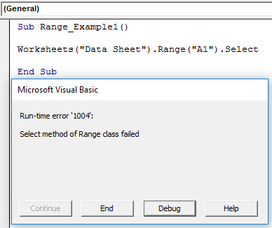
It is because “we cannot directly supply a range object and select method to the worksheets object.”

First, we need to select or activate the VBA worksheetWhen working with VBA, we frequently refer to or use the properties of another sheet. For instance, if we’re working on sheet 1 and need a value from cell A2 on sheet 2, we won’t be able to access it unless we first activate the sheet. So, to activate a sheet in VBA we use worksheet property as Worksheets(“Sheet2”). Activate.read more, and then we can do whatever we want.

Code:

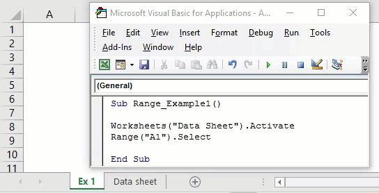
Sub Range_Example1()

  Worksheets("Data Sheet").Activate
  Range("A1").Select

End Sub

It will now select cell A1 in the worksheet “Data Sheet.”

Example #2 – Working with Current Selected Range

Selecting is different, and working with an already selected range of cells is different. For example, assume you want to insert a value “Hello VBA” to cell A1 then we can do it in two ways.

Firstly we can directly pass the VBA codeVBA code refers to a set of instructions written by the user in the Visual Basic Applications programming language on a Visual Basic Editor (VBE) to perform a specific task.read more as RANGE(“A1”).Value = “Hello, VBA.”

Code:

Sub Range_Example1()

  Range("A1").Value = "Hello VBA"

End Sub

This code will insert the value “Hello VBA” to cell A1, irrespective of which cell is currently selected.

Look at the above result of the code. When we execute this code, it has inserted the value “Hello VBA,” even though the currently selected cell is B2.

Secondly, we can insert the value into the cell using the “Selection” property. But, first, we need to select the cell manually and execute the code.

Code:

Sub Range_Example1()

  Selection.Value = "Hello VBA"

End Sub

What this code will do is insert the value “Hello VBA” to the currently selected cell. For example, look at the below example of execution.

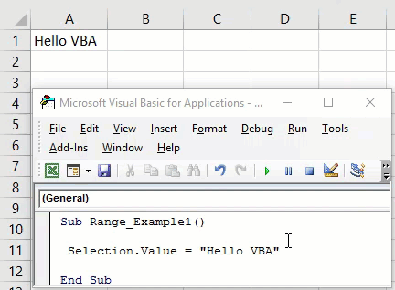
When we executed the code, my current selected cell was B2. Therefore, our code inserted the same value to the currently selected cell.

Now, we will select cell B3 and execute. There also, we will get the same value.

Another thing we can do with the “selection” property is insert a value to more than one cell. So, for example, we will select the range of cells from A1 to B5 now.

If we execute the code for all the selected cells, we get the value “Hello VBA.”

So, the simple difference between specifying a cell address by RANGE object and Selection property is that the Range object code will insert value to the cells specified explicitly.

But in the Selection object, it does not matter which cell you are in. It will insert the mentioned value to all the selected cells.

Things to Remember Here

We cannot directly supply the select method under the Selection property.
The RANGE is an object, and selection is property.
Instead of range, we can use the CELLS property.

Key Notes

You can use the Range property as well as Cells property to use the Select property to select a range.

Select a Single Cell

To select a single cell, you need to define the cell address using the range, and then you need to use the select property. Let’s say if you want to select cell A1, the code would be:

Range("A1").Select

And if you want to use the CELLS, in that case, the code would be:

Cells(1,1).Select

Select a Range of Cells

To select an entire range, you need to define the address of the range and then use the select property. For example, if you want to select the range A1 to A10, the code would be:

Range("A1:A10").Select

Select Non-Continues Range

To select a non-continuous range, you need to use a comma within the cell or range addresses, and then use the select the property. Let’s say if you want to select the range A1 to A10 and C5 to C10, the code would be:

Range("A1:A10, C5:C10").Select

And if you want to select single cells that are non-continuous, the code would be:

Range("A1, A5, A9").Select

Select a Column

To select a column, let’s say column A, you need to write code like the following:

Range("A:A").Select

And if you want to select multiple columns, in that case, the code would be like the following:

Range("A:C").Select
Range("A:A, C:C").Select

Select a Row

In the same way, if you want to select a row, let’s say row five, the code would be like the following.

Range("5:5").Select

And for multiple rows, the code would be:

Range("1:5").Select
Range("1:1, 3:3").Select

Select All the Cells of a Worksheet

Let’s say you want to select all the cells in the worksheet, just like you use the keyboard shortcut Control +A. You need to use the following code.

ActiveSheet.Cells.Select
Cells.Select

“Cells” refer to all the cells in the worksheet, and then select property selects them.

Select Cells with Data Only

Here “Cells with Data” only mean a section in the worksheet where cells have data and you can use the following code.

ActiveSheet.UsedRange.Select

Select a Named Range

If you have a named range, you can select it by using its name.

Range("my_range").Select

In the above code, you have the “my_range” named range and then the select property, and when you run this macro, it selects the specified range.

Select an Excel Table

If you work with Excel tables, you can also select them using the select property. Let’s say you have a table with the name “Data”, then the code to select that table would be:

If you want to select a column instead of the entire table, then the code would be, like the following:

Range("Data[Amount]").Select

And if you want to select the entire column including the header, then the code you can use:

Range("Data[[#All],[Amount]]").Select

You can also use the OFFSET property to select a cell or a range by navigating from a cell or a range. Let’s suppose you want to select a cell that is four columns right and five rows down from the A1; you can use the following code.

Range("A1").Offset(5, 4).Select

Excel VBA Selection Range

We all might have seen the process where we need to select the range so that we could perform some work on it. This is the basic step towards any task we do in Excel. If we do any manual work, then we can select the range of cells manually. But, while automating any process or work it is necessary to automate the process of Selection of Range as well. And VBA Selection Range is the basic steps toward any VBA code. When we write the steps for Selection of Range, their Range becomes the Object and Selection becomes the property. Which means the cells which we want to select are Objects and selection process of the property in VBA Selection Range.

How to Select a Range in Excel VBA?

We will learn how to select a range in Excel by using the VBA Code.

You can download this VBA Selection Range Excel Template here – VBA Selection Range Excel Template

Excel VBA Selection Range – Example #1

In the first example, we will see a very simple process where we will be selecting any range of cells using VBA code. For this, follow the below steps:

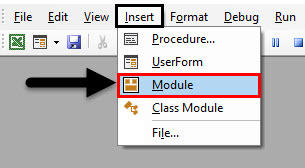
Step 1: Open a Module from the Insert menu tab where we will be writing the code for this.

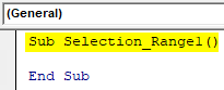
Step 2: Write the subcategory of VBA Selection Range or we can choose any other name as per our choice to define it.

Code:

Sub Selection_Range1()

End Sub

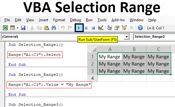
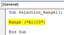
Step 3: Now suppose, we want to select the cells from A1 to C3, which forms a matrix box. Then we will write Range and in the brackets, we will put the cells which we want to select.

Code:

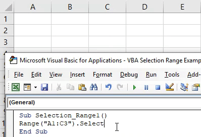
Sub Selection_Range1()

Range("A1:C3")

End Sub

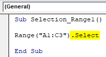
Step 4: Now we have covered the cells. Further, we can apply any function to it. We can select the cells, select the values it has or copy the selected range as well. Here we will simply select the range.

Code:

Sub Selection_Range1()

Range("A1:C3").Select

End Sub

Step 5: Now compile the code and run it by clicking on the Play button located below the menu bar. We will see the changes in the current sheet as cells from A1 to C3 are selected as shown below.

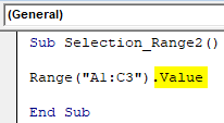
In a similar way, we can put any value to selected range cells. For this we will use Value function instead of Select.

Code:

Sub Selection_Range2()

Range("A1:C3").Value

End Sub

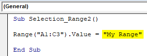
Now assign any value or text which we want to see in the selected range cells. Here that value is My Range.

Code:

Sub Selection_Range2()

Range("A1:C3").Value = "My Range"

End Sub

Now again run the code by clicking on the Play Button.

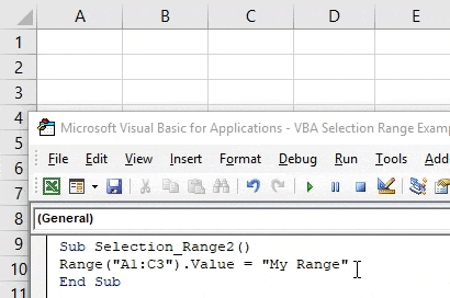
We will see the required text which we were in code value is got printed to the selected range.

Excel VBA Selection Range – Example #2

There is another way to implement VBA Selection Range. For this, follow the below steps:

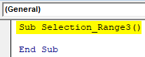
Step 1: Write the subcategory of VBA Selection Range as shown below.

Code:

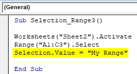
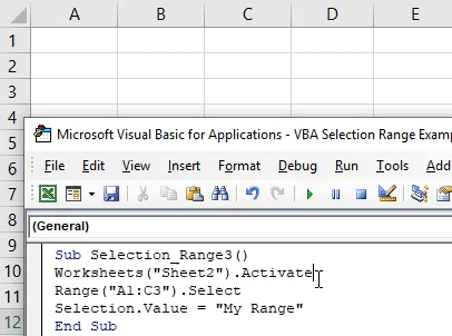
Sub Selection_Range3()

End Sub

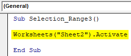
Step 2: By this process, we can select the range of any specific sheet which we want. We don’t need to make that sheet as current. Use Worksheet function to activate the sheet which wants by putting the name or sequence of the worksheet.

Code:

Sub Selection_Range3()

Worksheets("Sheet2").Activate

End Sub

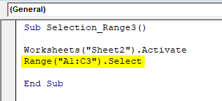
Step 3: Now again as per example-1, we will select the range of the cells which want to select. Here we are considering the same range from cell A1 to C3.

Code:

Sub Selection_Range3()

Worksheets("Sheet2").Activate
Range("A1:C3").Select

End Sub

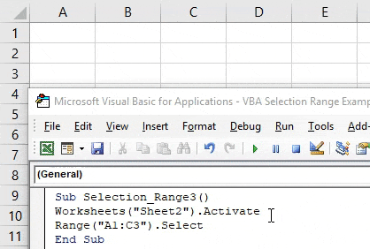
Step 4: Now run the code by clicking on the Play Button. We will see, the cells from A1 to C3 of the worksheet which is Name as Sheet2 are now selected.

As we have already selected the cells which we wanted, so now we can again write the one line code by which we will insert any text to selected cells. Or we can select the new range of cells manually also to see the changes by this code.

Step 5: For this use Selection function along with Value and choose the value which we want to see. Here our value is the same as we used before as My Range.

Code:

Sub Selection_Range3()

Worksheets("Sheet2").Activate
Range("A1:C3").Select
Selection.Value = "My Range"

End Sub

Step 6: Now again run the code by clicking on Play Button.

We will see, the selected cells from A1 to C3 got the value as My Range and those cells are still selected.

Excel VBA Selection Range – Example #3

In this example, we will see how to move the cursor from a current cell to the far most end cell. This process of selecting the end cell of the table or blank worksheet is quite useful in changing the location from where we can select the range. In Excel, this process is done manually by Ctrl + any Arrow key. Follow the below steps to use VBA Selection Range.

Step 1: Write the subcategory of VBA Selection Range again.

Code:

Sub Selection_Range4()

End Sub

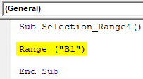
Step 2: Choose the reference range cell from where we want to move the cursor. Let’s say that cell is B1.

Code:

Sub Selection_Range4()

Range("B1")

End Sub

Step 3: Now to move to the End table or sheet towards right we will use xlToRight and for left it would be changed to xlToLeft as shown below.

Code:

Sub Selection_Range4()

Range("B1").End(xlToRight).Select

End Sub

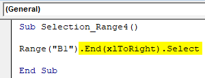
Step 4: Now run the code by pressing F5 key.

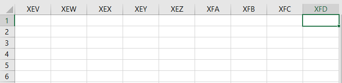
We will see, our cursor from anywhere from the first row or cell B1 will move to the far end to the sheet.

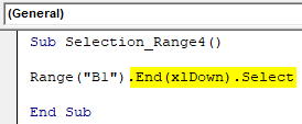
In a similar way, we can move the cursor and select the cell of the far down or up location of any sheet by xlDown or xlUP. Below is the code for selecting the far down cell of a sheet from reference cell B1.

Code:

Sub Selection_Range4()

Range("B1").End(xlDown).Select

End Sub

Pros of Excel VBA Selection Range

This is as easy as selecting the range of cells manually in Excel.
We can choose any type of range which we cannot do manually.
We can select and fill the cells which are only possible in excel by Find and Replace option.
Selecting the range cells and putting the data into that can be done simultaneously with one line of code.

Things to Remember

Using xlDown/Up and xlToLeft/Right command in code will take us to cells which is a far end or to the cell which has data. Means, the cell with the data will stop and prevent us from taking to the far end of the sheet.
We can choose any type of range but, make sure the range of cells is in sequence.
Random selection of cell is not allowed with these shown examples.
Always save the excel file as Macro Enable excel to prevent losing the code.

Video

About This Article

Is this article up to date?

Поиск по меткам

Table of contents

How to Select a Range in Excel VBA?

Example #1

Example #2 – Working with Current Selected Range

Things to Remember Here

Recommended Articles

Key Notes

Select a Single Cell

Select a Range of Cells

Select Non-Continues Range

Select a Column

Select a Row

Select All the Cells of a Worksheet

Select Cells with Data Only

Select a Named Range

Select an Excel Table

More Tutorials

Excel VBA Selection Range

How to Select a Range in Excel VBA?

Excel VBA Selection Range – Example #1

Excel VBA Selection Range – Example #2

Excel VBA Selection Range – Example #3

Pros of Excel VBA Selection Range

Things to Remember

Recommended Articles

A1: Name	B1: Sales	C1: Quantity
A2: a	B2: $10	C2: 5
A3: b	B3:	C3: 10
A4: c	B4: $10	C4: 5
A5:	B5:	C5:
A6: Total	B6: $20	C6: 20