
Свойства Row и Rows объекта Range в VBA Excel. Возвращение номера первой строки и обращение к строкам смежных и несмежных диапазонов.
Range.Row — свойство, которое возвращает номер первой строки в указанном диапазоне.
Свойство Row объекта Range предназначено только для чтения, тип данных — Long.
Если диапазон состоит из нескольких областей (несмежный диапазон), свойство Range.Row возвращает номер первой строки в первой области указанного диапазона:
|
Range(«B3:F10»).Select MsgBox Selection.Row ‘Результат: 3 Range(«E8:F9,D4:G13,B2:F10»).Select MsgBox Selection.Row ‘Результат: 8 |
Для возвращения номеров первых строк отдельных областей несмежного диапазона используется свойство Areas объекта Range:
|
Range(«E8:F9,D4:G13,B2:F10»).Select MsgBox Selection.Areas(1).Row ‘Результат: 8 MsgBox Selection.Areas(2).Row ‘Результат: 4 MsgBox Selection.Areas(3).Row ‘Результат: 2 |
Свойство Range.Rows
Range.Rows — свойство, которое возвращает объект Range, представляющий коллекцию строк в указанном диапазоне.
Чтобы возвратить одну строку заданного диапазона, необходимо указать ее порядковый номер (индекс) в скобках:
|
Dim myRange As Range Set myRange = Range(«B4:D6»).Rows(1) ‘Возвращается диапазон: $B$4:$D$4 Set myRange = Range(«B4:D6»).Rows(2) ‘Возвращается диапазон: $B$5:$D$5 Set myRange = Range(«B4:D6»).Rows(3) ‘Возвращается диапазон: $B$6:$D$6 |
Самое удивительное заключается в том, что выход индекса строки за пределы указанного диапазона не приводит к ошибке, а возвращается диапазон, расположенный за пределами исходного диапазона (отсчет начинается с первой строки заданного диапазона):
|
MsgBox Range(«B4:D6»).Rows(12).Address ‘Результат: $B$15:$D$15 |
Если указанный объект Range является несмежным, состоящим из нескольких смежных диапазонов (областей), свойство Rows возвращает коллекцию строк первой области заданного диапазона. Для обращения к строкам других областей указанного диапазона используется свойство Areas объекта Range:
|
Range(«E8:F9,D4:G13,B2:F10»).Select MsgBox Selection.Areas(1).Rows(2).Address ‘Результат: $E$9:$F$9 MsgBox Selection.Areas(2).Rows(2).Address ‘Результат: $D$5:$G$5 MsgBox Selection.Areas(3).Rows(2).Address ‘Результат: $B$3:$F$3 |
Определение количества строк в диапазоне:
|
Dim r As Long r = Range(«D4:K11»).Rows.Count MsgBox r ‘Результат: 8 |
Excel VBA Referencing Ranges — Range, Cells, Item, Rows & Columns Properties; Offset; ActiveCell; Selection; Insert
You can refer to or access a worksheet range using properties and methods of the Range object. A Range Object refers to a cell or a range of cells. It can be a row, a column or a selection of cells comprising of one or more rectangular / contiguous blocks of cells. One of the most important aspects in vba coding is referencing and using Ranges within a Worksheet. This section (divided into 2 parts) covers various properties and methods for referencing, accessing & using ranges, divided under the following chapters.
Excel VBA Referencing Ranges — Range, Cells, Item, Rows & Columns Properties; Offset; ActiveCell; Selection; Insert:
Range Property, Cells / Item / Rows / Columns Properties, Offset & Relative Referencing, Cell Address;
Activate & Select Cells; the ActiveCell & Selection;
Entire Row & Entire Column Properties, Inserting Cells/Rows/Columns using the Insert Method;
Excel VBA Refer to Ranges — Union & Intersect; Resize; Areas, CurrentRegion, UsedRange & End Properties; SpecialCells Method:
Ranges — Union & Intersect;
Resize a Range;
Referencing — Contiguous Block(s) of Cells, Range of Contiguous Data, Cells Meeting a Specified Criteria, Used Range, Cell at the End of a Block / Region, Last Used Row or Column;
Related Links:
Working with Objects in Excel VBA
Excel VBA Application Object, the Default Object in Excel
Excel VBA Workbook Object, working with Workbooks in Excel
Microsoft Excel VBA — Worksheets
Excel VBA Custom Classes and Objects
——————————————————————————————-
Contents:
Range Property, Cells / Item / Rows / Columns Properties, Offset & Relative Referencing, Cell Address
Activate & Select Cells; the ActiveCell & Selection
Entire Row & Entire Column Properties, Inserting Cells/Rows/Columns using the Insert Method
——————————————————————————————-
Range Property, Cells / Item / Rows / Columns Properties, Offset & Relative Referencing, Cell Address
A Range Object refers to a cell or a range of cells. It can be a row, a column or a selection of cells comprising of one or more rectangular / contiguous blocks of cells. A Range object is always with reference to a specific worksheet, and Excel currently does not support Range objects spread over multiple worksheets.
Range object refers to a single cell:
Dim rng As Range
Set rng = Range(«A1»)
Range object refers to a block of contiguous cells:
Dim rng As Range
Set rng = Range(«A1:C3»)
Range object refers to a row:
Dim rng As Range
Set rng = Rows(1)
Range object refers to multiple columns:
Dim rng As Range
Set rng = Columns(«A:C»)
Range object refers to 2 or more blocks of contiguous cells — using the ‘Union method’ & ‘Selection’ (these have been explained in detail later in this section).
Union method:
Dim rng1 As Range, rng2 As Range, rngUnion As Range
‘set a contiguous block of cells as the first range:
Set rng1 = Range(«A1:B2»)
‘set another contiguous block of cells as the second range:
Set rng2 = Range(«D3:E4»)
‘assign a variable (range object) to represent the union of the 2 ranges, using the Union method:
Set rngUnion = Union(rng1, rng2)
‘set interior color for the range which is the union of 2 range objects:
rngUnion.Interior.Color = vbYellow
Selection property:
‘select 2 contiguous block of cells, using the Select method:
Range(«A1:B2,D3:E4»).Select
‘perform action (set interior color of cells to yellow) on the Selection, which is a Range object:
Selection.Interior.Color = vbYellow
Range property of the Worksheet object ie. Worksheet.Range Property. Syntax: WorksheetObject.Range(Cell1, Cell2). You have an option to use only the Cell1 argument and in this case it will have to be a A1-style reference to a range which can include a range operator (colon) or the union operator (comma), or the reference to a range can be a defined name. Examples of using this type of reference are Worksheets(«Sheet1»).Range(«A1») which refers to cell A1; or Worksheets(«Sheet1»).Range(«A1:B3») which refers to the cells A1, A2, A3, B1, B2 & B3. When both the Cell1 & Cell2 arguments are used (cell1 and cell2 are Range objects), these refer to the cells at the top-left corner and the lower-right corner of the range (ie. the start and end cells of the range), and these arguments can be a single cell, an entire row or column or a single named cell. An example of using this type of reference is Worksheets(«Sheet1»).Range(Cells(1, 1), Cells(3, 2)) which refers to the cells A1, A2, A3, B1, B2 & B3. Omitting the object qualifier will default to the active sheet viz. using the code Range(«A1») will return cell A1 of the active sheet, and will be the same as using Application.Range(«A1») or ActiveSheet.Range(«A1»).
Range property of the Range object: Use the Range.Range property [Syntax: RangeObject.Range(Cell1,Cell2)] for relative referencing ie. to access a range relative to a range object. For example, Worksheets(«Sheet1»).Range(«C5:E8»).Range(«A1») will refer to Range(«C5») and Worksheets(«Sheet1»).Range(«C5:E8»).Range(«B2») will refer to Range(«D6»).
Shortcut Range Reference: As compared to using the Range property, you can also use a shorter code to refer to a range by using square brackets to enclose an A1-style reference or a name. While using square brackets, you do not type the Range word or wrap the range in quotation marks to make it a string. Using square brackets is similar to applying the Evaluate method of the Application object. The Range property or the Evaluate method use a string argument which enables you to manipulate the string with vba code, whereas using the square brackets will be inflexible in this respect. Examples: using [A1].Value = 5 is equivalent to using Range(«A1»).Value = 5; using [A1:A3,B2:B4,C3:D5].Interior.Color = vbRed is equivalent to Range(«A1:A3,B2:B4,C3:D5»).Interior.Color = vbRed; and with named ranges, [Score].Interior.Color = vbBlue is equivalent to Range(«Score»).Interior.Color = vbBlue. Using square brackets only enables reference to fixed ranges which is a significant shortcoming. Using the Range property enables you to manipulate the string argument with vba code so that you can use variables to refer to a dynamic range, as illustrated below:
Sub DynamicRangeVariable()
‘using a variable to refer a dynamic range.
Dim i As Integer
‘enters the text «Hello» in each cell from B1 to B5:
For i = 1 To 5
Range(«B» & i) = «Hello»
Next
End Sub
The Cells Property returns a Range object referring to all cells in a worksheet or a range, as it can be used with respect to an Application object, a Worksheet object or a Range object. Application.Cells Property refers to all cells in the active worksheet. You can use the code Application.Cells or omit the object qualifier (this property is a member of ‘globals’) and use the code Cells to refer to all cells of the active worksheet. The Worksheet.Cells Property (Syntax: WorksheetObject.Cells) refers to all cells of a specified worksheet. Use the code Worksheets(«Sheet1»).Cells to refer to all cells of worksheet named «Sheet1». Use the Range.Cells Property ro refer to cells in a specified range — (Syntax: RangeObject.Cells). This property can be used as Range(«A1:B5»).Cells, however using the word cells in this case is immaterial because with or without this word the code will refer to the range A1:B5. To refer to a specific cell, use the Item property of the Range object (as explained in detail below) by specifying the relative row and column positions after the Cells keyword, viz. Worksheets(«Sheet1»).Cells.Item(2, 3) refers to range C2 and Worksheets(«Sheet1»).Range(«C2»).Cells(2, 3) will refer to range E3. Because the Item property is the Range object’s default property you can omit the Item word word and use the code Worksheets(«Sheet1»).Cells(2, 3) which also refers to range C2. You may find it preferable in some cases to use Worksheets(«Sheet1»).Cells(2, 3) over Worksheets(«Sheet1»).Range(«C2») because variables for the row and column can easily be used therein.
Item property of the Range object: Use the Range.Item Property to return a range as offset to the specified range. Syntax: RangeObject.Item(RowIndex, ColumnIndex). The Item word can be omitted because Item is the Range object’s default property. It is necessary to specify the RowIndex argument while ColumnIndex is optional. RowIndex is the index number of the cell, starting with 1 and increasing from left to right and then down. Worksheets(«Sheet1»).Cells.Item(1) or Worksheets(«Sheet1»).Cells(1) refers to range A1 (the top-left cell in the worksheet), Worksheets(«Sheet1»).Cells(2) refers to range B1 (cell next to the right of the top-left cell). While using a single-parameter reference of the Item property (ie. RowIndex), if index exceeds the number of columns in the specified range, the reference will wrap to successive rows within the range columns. Omitting the object qualifier will default to active sheet. Cells(16385) refers to range A2 of the active sheet in Excel 2007 which has 16384 columns, and Cells(16386) refers to range B2, and so on. Also note that RowIndex and ColumnIndex are offsets and relative to the specified Range (ie. relative to the top-left corner of the specified range). Both Range(«B3»).Item(1) and Range(«B3:D6»).Item(1) refer to range B3. The following refer to range D4, the sixth cell in the range: Range(«B3:D6»).Item(6) or Range(«B3:D6»).Cells(6) or Range(«B3:D6»)(6). ColumnIndex refers to the column number of the cell, can be a number starting with 1 or can be a string starting with the letter «A». Worksheets(«Sheet1»).Cells(2, 3) and Worksheets(«Sheet1»).Cells(2, «C») both refer to range C2 wherein the RowIndex is 2 and ColumnIndex is 3 (column C). Range(«C2»).Cells(2, 3) refers to range E3 in the active sheet, and Range(«C2»).Cells(4, 5) refers to range G5 in the active sheet. Using Range(«C2»).Item(2, 3) and Range(«C2»).Item(4, 5) has the same effect and will refer to range E3 & range G5 respectively. Using Range(«C2:D3»).Cells(2, 3) and Range(«C2:D3»).Cells(4, 5) will also refer to range E3 & range G5 respectively. Omitting the Item or Cells word — Range(«C2:D3»)(2, 3) and Range(«C2:D3»)(4, 5) also refers to range E3 & range G5 respectively. It is apparant here that you can refer to and return cells outside the original specified range, using the Item property.
Columns property of the Worksheet object: Use the Worksheet.Columns Property (Syntax: WorksheetObject.Columns) to refer to all columns in a worksheet which are returned as a Range object. Example: Worksheets(«Sheet1»).Columns will return all columns of the worksheet; Worksheets(«Sheet1»).Columns(1) returns the first column (column A) in the worksheet; Worksheets(«Sheet1»).Columns(«A») returns the first column (column A); Worksheets(«Sheet1»).Columns(«A:C») returns the columns A, B & C; and so on. Omitting the object qualifier will default to the active sheet viz. using the code Columns(1) will return the first column of the active sheet, and will be the same as using Application.Columns(1).
Columns property of the Range object: Use the Range.Columns Property (Syntax: RangeObject.Columns) to refer to columns in a specified range. Example1: color cells from all columns of the specified range ie. B2 to D4: Worksheets(«Sheet1»).Range(«B2:D4»).Columns.Interior.Color = vbYellow. Example2: color cells from first column of the range only ie. B2 to B4: Worksheets(«Sheet1»).Range(«B2:D4»).Columns(1).Interior.Color = vbGreen. If the specified range object contains multiple areas, the columns from the first area only will be returned by this property (Areas property has been explained in detail later in this section). Take the example of 2 areas in the specified range, first area being «B2:D4» and the second area being «F3:G6» — the following code will color cells from first column of the first area only ie. cells B2 to B4: Worksheets(«Sheet1»).Range(«B2:D4, F3:G6»).Columns(1).Interior.Color = vbRed. Omitting the object qualifier will default to active sheet — following will apply color to column A of the ActiveSheet: Columns(1).Interior.Color = vbRed.
Use the Worksheet.Rows Property (Syntax: WorksheetObject.Rows) to refer to all rows in a worksheet which are returned as a Range object. Example: Worksheets(«Sheet1»).Rows will return all rows of the worksheet; Worksheets(«Sheet1»).Rows(1) returns the first row (row one) in the worksheet; Worksheets(«Sheet1»).Rows(3) returns the third row (row three) in the worksheet; Worksheets(«Sheet1»).Rows(«1:3») returns the first 3 rows; and so on. Omitting the object qualifier will default to the active sheet viz. using the code Rows(1) will return the first row of the active sheet, and will be the same as using Application.Rows(1).
Use the Range.Rows Property (Syntax: RangeObject.Rows) to refer to rows in a specified range. Example1: color cells from all rows of the specified range ie. B2 to D4: Worksheets(«Sheet1»).Range(«B2:D4»).Rows.Interior.Color = vbYellow. Example2: color cells from first row of the range only ie. B2 to D2: Worksheets(«Sheet1»).Range(«B2:D4»).Rows(1).Interior.Color = vbGreen. If the specified range object contains multiple areas, the rows from the first area only will be returned by this property (Areas property has been explained in detail later in this section). Take the example of 2 areas in the specified range, first area being «B2:D4» and the second area being «F3:G6» — the following code will color cells from first row of the first area only ie. cells B2 to D2: Worksheets(«Sheet1»).Range(«B2:D4, F3:G6»).Rows(1).Interior.Color = vbRed. Omitting the object qualifier will default to active sheet — following will apply color to row one of the ActiveSheet: Rows(1).Interior.Color = vbRed.
To refer to a range as offset from a specified range, use the Range.Offset Property. Syntax: RangeObject.Offset(RowOffset, ColumnOffset). Both arguments are optional to specify. The RowOffset argument specifies the number of rows by which the specified range is offset — negative values indicating upward offset and positive values indicating downward offset, with default value being 0. The ColumnOffset argument specifies the number of columns by which the specified range is offset — negative values indicating left offset and positive values indicating right offset, with default value being 0. Examples: Range(«C5»).Offset(1, 2) offsets 1 row & 2 columns and refers to Range E6, Range(«C5:D7»).Offset(1, -2) offsets 1 row downward & 2 columns to the left and refers to Range (A6:B8).
Accessing a worksheet range, with vba code:-
Referencing a single cell:
Enter the value 10 in the cell A1 of the worksheet named «Sheet1» (omitting to mention a property with the Range object will assume the Value property, as shown below):
Worksheets(«Sheet1»).Range(«A1»).Value = 10
Worksheets(«Sheet1»).Range(«A1») = 10
Enter the value of 10 in range C2 of the active worksheet — using Cells(row, column) where row is the row index and column is the column index:
ActiveSheet.Cells(2, 3).Value = 10
Referencing a range of cells:
Enter the value 10 in the cells A1, A2, A3, B1, B2 & B3 (wherein the cells refer to the upper-left corner & lower-right corner of the range) of the active sheet:
ActiveSheet.Range(«A1:B3»).Value = 10
ActiveSheet.Range(«A1», «B3»).Value = 10
ActiveSheet.Range(Cells(1, 1), Cells(3, 2)) = 10
Enter the value 10 in the cells A1 & B3 of worksheet named «Sheet1»:
Worksheets(«Sheet1»).Range(«A1,B3»).Value = 10
Set the background color (red) for cells B2, B3, C2, C3, D2, D3 & H7 of worksheet named «Sheet3»:
ActiveWorkbook.Worksheets(«Sheet3»).
Range(«B2:D3,H7»).Interior.Color = vbRed
Enter the value 10 in the Named Range «Score» of the active worksheet, viz. you can name the Range(«B2:B3») as «Score» to insert 10 in the cells B2 & B3:
Range(«Score»).Value = 10
ActiveSheet.Range(«Score»).Value = 10
Select all the cells of the active worksheet:
ActiveSheet.Cells.Select
Cells.Select
Set the font to «Times New Roman» & the font size to 11, for all the cells of the active worksheet in the active workbook:
ActiveWorkbook.ActiveSheet.Cells.Font.Name = «Times New Roman»
ActiveSheet.Cells.Font.Size = 11
Cells.Font.Size = 11
Referencing Row(s) or Column(s):
Select all the Rows of active worksheet:
ActiveSheet.Rows.Select
Enter the value 10 in the Row number 2 (ie. every cell in second row), of worksheet named «Sheet1»:
Worksheets(«Sheet1»).Rows(2).Value = 10
Select all the Columns of the active worksheet:
ActiveSheet.Columns.Select
Columns.Select
Enter the value 10 in the Column number 3 (ie. every cell in column C), of the active worksheet:
ActiveSheet.Columns(3).Value = 10
Columns(«C»).Value = 10
Enter the value 10 in Column numbers 1, 2 & 3 (ie. every cell in columns A to C), of worksheet named «Sheet1»:
Worksheets(«Sheet1»).Columns(«A:C»).Value = 10
Relative Referencing:
Inserts the value 10 in Range C5 — reference starts from upper-left corner of the defined Range:
Range(«C5:E8»).Range(«A1») = 10
Inserts the value 10 in Range D6 — reference starts from upper-left corner of the defined Range:
Range(«C5:E8»).Range(«B2») = 10
Inserts the value 10 in Range E6 — offsets 1 row & 2 columns, using the Offset property:
Range(«C5»).Offset(1, 2) = 10
Inserts the value 10 in Range(«F7:H10») — offsets 2 rows & 3 columns, using the Offset property:
Range(«C5:E8»).Offset(2, 3) = 10
Example 1 — Using Range, Cells, Columns & Rows property — refer Image 1:

Sub CellsColumnsRowsProperty()
‘using Range, Cells, Columns & Rows property — refer Image 1:
Dim ws As Worksheet
Dim rng As Range
Dim r As Integer, c As Integer, n As Integer, i As Integer, j As Integer
‘set worksheet:
Set ws = Worksheets(«Sheet1»)
‘activate worksheet:
ws.activate
‘enter numbers starting from 1 in each row, for a 5 row & 5 column range (A1:E5):
For r = 1 To 5
n = 1
For c = 1 To 5
Cells(r, c).Value = n
n = n + 1
Next c
Next r
‘set range to A1:E5, wherein the numbers have been entered as above:
Set rng = Range(Cells(1, 1), Cells(5, 5))
‘set background color of each even number column to yellow and of each odd number column to green:
For i = 1 To 5
If i Mod 2 = 0 Then
rng.Columns(i).Interior.Color = vbYellow
Else
rng.Columns(i).Interior.Color = vbGreen
End If
Next i
‘set font color to red and set font to bold for of even number rows:
For j = 1 To 5
If j Mod 2 = 0 Then
rng.Rows(j).Font.Bold = True
rng.Rows(j).Font.Color = vbRed
End If
Next j
‘set font for all cells of the range to italics:
rng.Cells.Font.Italic = True
End Sub
To return the number of the first row in a range, use the Range.Row Property. If the specified range contains multiple areas, this property will return the number of the first row in the first area (Areas property has been explained in detail later in this section). Syntax: RangeObject.Row. To return the number of the first column in a range, use the Range.Column Property. If the specified range contains multiple areas, this property will return the number of the first column in the first area. Syntax: RangeObject.Column.
Examples:
Get the number of the first row in the specified range — returns 4:
MsgBox ActiveSheet.Range(«B4»).Row
MsgBox Worksheets(«Sheet1»).Range(«B4:D7»).Row
Get the number of the first column in the specified range — returns 2:
MsgBox ActiveSheet.Range(«B4:D7»).Column
Get the number of the last row in the specified range — returns 7:
Explanation: Range(«B4:D7»).Rows.Count returns 4 (the number of rows in the range). Range(«B4:D7»).Rows(Range(«B4:D7»).Rows.Count) or Range(«B4:D7»).Rows(4), returns the last row in the specified range.
MsgBox Range(«B4:D7»).Rows(Range(«B4:D7»).
Rows.Count).Row
Example 2: Using Row Property, Column Property & Rows Property, determine row number & column number, and alternate rows — refer Image 2.

Sub RowColumnProperty()
‘Using Row Property, Column Property & Rows Property, determine row number & column number, and alternate rows — refer Image 2.
Dim rng As Range, cell As Range
Dim i As Integer
Set rng = Worksheets(«Sheet1»).Range(«B4:D7»)
‘enter its row number & column number within each cell in the specified range:
For Each cell In rng
cell.Value = cell.Row & «,» & cell.Column
Next
‘set background color of each alternate row of the specified range:
For i = 1 To rng.Rows.count
If i Mod 2 = 1 Then
rng.Rows(i).Interior.Color = vbGreen
Else
rng.Rows(i).Interior.Color = vbYellow
End If
Next
End Sub
Also refer to Example 23, of using the End & Row properties to determine the last used row or column with data.
You can get a Range reference in vba language by using the Range.Address Property, which returns the address of a Range as a string value. This property is read-only.
Examples of using the Address Property:
Returns $B$2:
MsgBox Range(«B2»).Address
Returns $B$2,$C$3:
MsgBox Range(«B2,C3»).Address
Returns $A$1:$B$2,$C$3,$D$4:
Dim strRng As String
Range(«A1:B2,C3,D4»).Select
strRng = Selection.Address
MsgBox strRng
Returns $B2:
MsgBox Range(«B2»).Address(RowAbsolute:=False)
Returns B$2:
MsgBox Range(«B2»).Address(ColumnAbsolute:=False)
Returns R2C2:
MsgBox Range(«B2»).Address(ReferenceStyle:=xlR1C1)
Includes the worksheet (active sheet — «Sheet1») & workbook («Book1.xlsm») name, and returns [Book1.xlsm]Sheet1!$B$2:
MsgBox Range(«B2»).Address(External:=True)
Returns R[1]C[-1] — Range(«B2») is 1 row and -1 columns relative to Range(«C1»):
MsgBox Range(«B2»).Address(RowAbsolute:=False, ColumnAbsolute:=False, ReferenceStyle:=xlR1C1, RelativeTo:=Range(«C1»))
Returns RC[-2] — Range(«A1») is 0 row and -2 columns relative to Range(«C1»):
MsgBox Cells(1, 1).Address(RowAbsolute:=False, ColumnAbsolute:=False, ReferenceStyle:=xlR1C1, RelativeTo:=Range(«C1»))
Activate & Select Cells; the ActiveCell & Selection
The Select method (of the Range object) is used to select a cell or a range of cells in a worksheet — Syntax: RangeObject.Select. Ensure that the worksheet wherein the Select method is applied to select cells, is the active sheet. The ActiveCell Property (of the Application object) returns a single active cell (Range object) in the active worksheet. Remember that the ActiveCell property will not work if the active sheet is not a worksheet. When a cell(s) is selected in the active window, the Selection property (of the Application object) returns a Range object representing all cells which are currently selected in the active worksheet. A Selection may consist of a single cell or a range of multiple cells, but there will only be one active cell within it, which is returned by using the ActiveCell property. When only a single cell is selected, the ActiveCell property returns this cell. On selecting multiple cells using the Select method, the first referenced cell becomes the active cell, and thereafter you can change the active cell using the Activate method. Both the ActiveCell Property & the Selection property are read-only, and not specifying the Application object qualifier viz. Application.ActiveCell or ActiveCell, Application.Selection or Selection, will have the same effect. To activate a single cell within the current selection, use the Activate Method (of the Range object) — Syntax: RangeObject.Activate, and this activated cell is returned by using the ActiveCell property.
We have discussed above that a Selection may consist of a single cell or a range of multiple cells, whereas there can be only one active cell within the Selection. When you activate a cell outside the current selection, the activated cell becomes the only selected cell. You can also use the Activate method to specify a range of multiple cells, but in effect only a single cell will be activated, and this activated cell will be the top-left corner cell of the range specified in the method. If this top-left cell lies within the selection, the current selection will not change, but if this top-left cell lies outside the selection, then the specified range in the Activate method becomes the new selection.
See below codes which illustrate the concepts of ActiveCell and Selection.
Selection containing a range of cells, and the active cell:
‘selects range C1:F5:
Range(«C1:F5»).Select
‘returns C1, the first referenced cell, as the active cell:
MsgBox ActiveCell.Address
Selection containing a range of cells, and the active cell:
‘selects range C1:F5:
Range(«F5:C1»).Select
‘returns C1, the first referenced cell, as the active cell:
MsgBox ActiveCell.Address
Selection containing a range of cells, and the active cell:
‘selects range C1:F5:
Range(«C5:F1»).Select
‘returns C1, the first referenced cell, as the active cell:
MsgBox ActiveCell.Address
Activate a cell within the current selection:
‘selects range B6:F10:
Range(«B6:F10»).Select
‘returns B6, the first referenced cell, as the active cell:
MsgBox ActiveCell.Address
‘selection remains same — range B6:F10, but the active cell is now C8:
Range(«C8»).Activate
MsgBox ActiveCell.Address
Activate a cell outside the current selection:
‘selects range B6:F10:
Range(«B6:F10»).Select
‘returns B6, the first referenced cell, as the active cell:
MsgBox ActiveCell.Address
‘both the selection and the active cell is now A2:
Range(«A2»).Activate
MsgBox ActiveCell.Address
Select a cell within the current selection:
‘selects range B6:F10:
Range(«B6:F10»).Select
‘returns B6, the first referenced cell, as the active cell:
MsgBox ActiveCell.Address
‘both the selection and the active cell is now C8:
Range(«C8»).Select
MsgBox ActiveCell.Address
Activate a range of cells whose top-left cell is within the current selection:


‘selects range B6:F10 — refer Image 3a:
Range(«B6:F10»).Select
‘returns B6, the first referenced cell, as the active cell:
MsgBox ActiveCell.Address
‘selection remains same — range B6:F10, but the active cell is now C8 — refer Image 3b:
Range(«C8:G12»).Activate
MsgBox ActiveCell.Address
Activate a range of cells whose top-left cell is outside the current selection:

‘selects range B6:F10 — refer Image 3a:
Range(«B6:F10»).Select
‘returns B6, the first referenced cell, as the active cell:
MsgBox ActiveCell.Address
‘selection range changes to range B1:F8, and the active cell is now B1 — refer Image 3c:
Range(«B1:F8»).Activate
MsgBox ActiveCell.Address
Using the Application.Selection Property returns the selected object wherein the selection determines the returned object type. Where the selection is a range of cells, this property returns a Range object, and this Selection — which is a Range object — can comprise of a single cell, or multiple cells or multiple non-contiguous ranges. And as mentioned above, the Select method (of the Range object) is used to select a cell or a range of cells in a worksheet. Therefore, after selecting a range, you can perform actions on the selection of cells by using the Selection object. See below illustration.
Sub SelectionObject()
‘select cells in the active sheet using the Range.Select method:
Range(«A1:B3,D6»).Select
‘perform action (set interior color of cells to red) on the Selection, which is a Range object:
Selection.Interior.Color = vbRed
End Sub
Entire Row & Entire Column Properties, Inserting Cells/Rows/Columns using the Insert Method
Use the Range.EntireRow Property to return an entire row or rows within which the specific range is contained. Using this property returns a Range object referring to the entire row(s). Syntax: RangeObject.EntireRow. Use the Range.EntireColumn Property to return an entire column or columns within which the specific range is contained. Using this property returns a Range object referring to the entire column(s). Syntax: RangeObject.EntireColumn.
Examples of using the EntireRow & EntireColumn Properties
Selects row no. 2:
Range(«A2»).EntireRow.Select
Selects row nos. 2, 3 & 4:
Range(«A2:C4»).EntireRow.Select
Enters value 3 in range A3 ie. in the first cell of row no. 3:
Cells(3, 4).EntireRow.Cells(1, 1).Value = 3
Selects column A:
Range(«A2»).EntireColumn.Select
Selects columns A to C:
Range(«A2:C4»).EntireColumn.Select
Enters value 4 in range D1 ie. in the first cell of column no. 4:
Cells(3, 4).EntireColumn.Cells(1, 1).Value = 4
Use the Range.Insert Method to insert a cell or a range of cells in a worksheet. Syntax: RangeObject.Insert(Shift, CopyOrigin). Both arguments are optional to specify. When you insert cell(s) the other cells are shifted to make way, and you can set a value for the Shift argument to determine the direction in which the other cells are shifted — specifying xlShiftDown (value -4121) will shift the cells down, and xlShiftToRight (value -4161) shifts the cells to the right. Omitting this argument will decide the shift direction based on the shape of the range. Specifying xlFormatFromLeftOrAbove (value 0) for the CopyOrigin argument will copy the format for inserted cell(s) from the above cells or cells to the left, and specifying xlFormatFromRightOrBelow (value 1) will copy format from the below cells or cells to the right.
Illustrating Range.Insert Method — for start data refer Image 4a:


Shifts cells down and copies formatting of inserted cell from above cell — refer image 4b:
Range(«B2»).Insert

Shifts cells to the right and copies formatting of inserted cells from cells to the left — refer image 4c:
Range(«B2:C4»).Insert

Shifts cells down and copies formatting of inserted cells from above cells — refer image 4d:
Range(«B2:D3»).Insert

Shifts cells down and copies formatting of inserted cells from below cells — refer image 4e:
Range(«B2:D3»).Insert CopyOrigin:=xlFormatFromRightOrBelow

Shifts cells to the right and copies formatting of inserted cells from cells to the left — refer image 4f:
Range(«B2:D3»).Insert shift:=xlShiftToRight

Shifts cells to the right and copies formatting of inserted cells from cells to the right — refer image 4g:
Range(«B2:D3»).Insert shift:=xlShiftToRight, CopyOrigin:=xlFormatFromRightOrBelow

Inserts 2 rows — row no 2 & 3 — and copies formatting of inserted rows from above cells — refer image 4h:
Range(«B2:D3»).EntireRow.Insert
Below are some illustrations of inserting entire row(s) or column(s) dynamically in a worksheet.
Example 3: Insert row or column — specify the row / column to insert.
Sub InsertRowColumn()
‘Insert row or column — specify the row / column to insert:
Dim ws As Worksheet
Set ws = Worksheets(«Sheet1»)
‘NOTE: each of the below codes need to be run individually.
‘specify the exact row number to insert — insert a row as row no 12:
ws.Rows(12).Insert
‘specify the range below which to insert a row — insert a row below range C3 ie. as row no 4.
ws.Range(«C3»).EntireRow.Offset(1, 0).Insert
‘specify the exact column number to insert — insert a column as column no 4:
ws.Columns(4).Insert
‘specify the range to the right of which to insert a column — insert a column to the right of range C3 ie. as column no 4.
ws.Range(«C3»).EntireColumn.Offset(0, 1).Insert
End Sub
Example 4: Insert row(s) after a specified value is found.
Sub InsertRow1()
‘insert row(s) after a specified value is found:
Dim ws As Worksheet
Dim rngFind As Range, rngSearch As Range, rngLastCell As Range
Dim lFindRow As Long
Set ws = Worksheets(«Sheet1»)
‘find a value after which to insert a row:
Set rngSearch = ws.Range(«A1:E100»)
‘begin search AFTER the last cell in search range (this will start serach from the first cell in search range):
Set rngLastCell = rngSearch.Cells(rngSearch.Cells.count)
Set rngFind = rngSearch.Find(What:=«ExcelVBA», After:=rngLastCell, LookIn:=xlValues, lookat:=xlWhole)
‘exit procedure if value not found:
If Not rngFind Is Nothing Then
lFindRow = rngFind.Row
MsgBox lFindRow
Else
MsgBox «Value not found!»
Exit Sub
End If
‘NOTE: each of the below codes need to be run individually.
‘if value found is in row no 12, one row will be inserted below as row no 13:
ws.Cells(lFindRow + 1, 1).EntireRow.Insert
‘if value found is in row no 12, one row will be inserted 3 rows below (as row no 15):
ws.Cells(lFindRow + 3, 1).EntireRow.Insert
‘if value found is in row no 12, one row will be inserted 3 rows below (as row no 15):
ws.Cells(lFindRow, 1).Offset(3).EntireRow.Insert
‘if value found is in row no 12, 3 rows will be inserted above (as row nos 12, 13 & 14) and the value found row 12 will be pushed down to row 15:
ws.Cells(lFindRow, 1).EntireRow.Resize(3).Insert
‘alternate:
ws.Range(Cells(lFindRow, 1), Cells(lFindRow + 2, 1)).EntireRow.Insert
‘alternate:
ws.Rows(lFindRow & «:» & lFindRow + 2).EntireRow.Insert Shift:=xlDown
‘if value found is in row no 12, 3 rows will be inserted below (as row nos 13, 14 & 15) and the value found row 12 will remain at the same position:
ws.Cells(lFindRow + 1, 1).EntireRow.Resize(3).Insert
‘alternate:
ws.Range(ws.Cells(lFindRow + 1, 1), ws.Cells(lFindRow + 3, 1)).EntireRow.Insert
‘if value found is in row no 12, 3 rows will be inserted after row no 13 (as row nos 14, 15 & 16) and existing rows 12 & 13 will remain at the same position:
ws.Cells(lFindRow + 2, 1).EntireRow.Resize(3).Insert
End Sub
Example 5: Insert a row, n rows above the last used row.
Sub InsertRow2()
‘insert a row, n rows above the last used row
Dim ws As Worksheet
Dim lRowsC As Long
Set ws = Worksheets(«Sheet1»)
‘determine the last used row in a column (column A):
lRowsC = ws.Cells(Rows.count, «A»).End(xlUp).Row
MsgBox lRowsC
‘set n to the no of rows above the last used row:
n = 5
‘check if there are enough rows before the last used row, else you will get an error:
If lRowsC >= n Then
‘insert a row, n rows above the last used row — if last used row is no 5 before insertion, then insert as row no 1 and the last used row will become no 6 (similarly, if last used row is 27, then insert as row no 23) :
ws.Rows(lRowsC).Offset(-n + 1, 0).EntireRow.Insert
Else
MsgBox «Not enough rows before the last used row!»
End If
End Sub
Example 6: Insert a row each time the searched value is found in a range.
For live code of this example, click to download excel file.
Sub InsertRow3()
‘search value in a range and insert a row each time the value is found.
‘you can set the search range with the variable rngSearch in below code — the code will look within this range to find the value below which row is to be inserted.
Dim ws As Worksheet
Dim rngFind As Range, rngSearch As Range, rngLastCell As Range
Dim strAddress As String
Set ws = Worksheets(«Sheet1»)
‘set search range:
Set rngSearch = ws.Range(«A1:K100»)
MsgBox «Searching for ‘ExcelVBA’ within range: » & rngSearch.Address
‘begin search AFTER the last cell in search range
Set rngLastCell = rngSearch.Cells(rngSearch.Cells.count)
‘find value in specified range, starting search AFTER the last cell in search range:
Set rngFind = rngSearch.Find(What:=«ExcelVBA», After:=rngLastCell, LookIn:=xlValues, lookat:=xlWhole)
If rngFind Is Nothing Then
MsgBox «Value not found!»
Exit Sub
Else
‘save cell address of first value found:
strAddress = rngFind.Address
Do
‘find next occurrence of value:
Set rngFind = rngSearch.FindNext(After:=rngFind)
‘insert row below when value is found (if value is found twice in a row, then 2 rows will be inserted):
rngFind.Offset(1).EntireRow.Insert
‘loop till reaching the first value found range:
Loop While rngFind.Address <> strAddress
End If
End Sub
Example 7: Insert rows (user-defined number) within consecutive values found in a column — refer Images 5a & 5b.
For live code of this example, click to download excel file.


Sub InsertRow4()
‘insert rows (user-defined number) wherever 2 consecutive values are found in a column.
‘set column number in which 2 consecutive values are checked to insert rows, using the variable lCellColumn in below code.
‘set row number from where to start searching consecutive values, using the variable lCellRow in below code.
‘refer Image 5a which shows raw data, and Image 5b after this procedure is executed — a single row (lRowsInsert value entered as 1 in input box) is inserted where consecutive values appear in column 1:
Dim ws As Worksheet
Dim lLastUsedRow As Long, lRowsInsert As Long, lCellRow As Long, lCellColumn As Long
Dim rng As Range
Set ws = Worksheets(«Sheet1»)
ws.Activate
‘set column number in which 2 consecutive values are checked to insert rows:
lCellColumn = 1
‘set row number from where to start searching consecutive values:
lCellRow = 1
‘determine the last used row in the column (column no. lCellColumn):
lLastUsedRow = Cells(Rows.count, lCellColumn).End(xlUp).Row
‘enter number of rows to insert between 2 consecutive values:
lRowsInsert = InputBox(«Enter number of rows to insert»)
If lRowsInsert < 1 Then
MsgBox «Error — please enter a value equal to or greater than 1»
Exit Sub
End If
MsgBox «This code will insert » & lRowsInsert & » rows, wherever consecutive values are found in column number » & lCellColumn & «, starting search from row number » & lCellRow
‘loop till the row number equals the last used row (ie. loop right till the end value in the column):
Do While lCellRow < lLastUsedRow
Set rng = Cells(lCellRow, lCellColumn)
‘in case of 2 consecutive values:
If rng <> «» And rng.Offset(1, 0) <> «» Then
‘enter the user-defined number of rows:
Range(rng.Offset(1, 0), rng.Offset(lRowsInsert, 0)).EntireRow.Insert
lCellRow = lCellRow + lRowsInsert + 1
‘determine the last used row — it is dynamic and changes on insertion of rows:
lLastUsedRow = Cells(Rows.count, lCellColumn).End(xlUp).Row
‘alternate method to determine the last used row, when number of rows inserted is fixed — this is faster than using End(xlUp):
‘lLastUsedRow = lLastUsedRow + lRowsInsert + 1
‘MsgBox lLastUsedRow
Else
lCellRow = lCellRow + 1
End If
Loop
End Sub
“It is a capital mistake to theorize before one has data”- Sir Arthur Conan Doyle
This post covers everything you need to know about using Cells and Ranges in VBA. You can read it from start to finish as it is laid out in a logical order. If you prefer you can use the table of contents below to go to a section of your choice.
Topics covered include Offset property, reading values between cells, reading values to arrays and formatting cells.
A Quick Guide to Ranges and Cells
| Function | Takes | Returns | Example | Gives |
|---|---|---|---|---|
|
Range |
cell address | multiple cells | .Range(«A1:A4») | $A$1:$A$4 |
| Cells | row, column | one cell | .Cells(1,5) | $E$1 |
| Offset | row, column | multiple cells | Range(«A1:A2») .Offset(1,2) |
$C$2:$C$3 |
| Rows | row(s) | one or more rows | .Rows(4) .Rows(«2:4») |
$4:$4 $2:$4 |
| Columns | column(s) | one or more columns | .Columns(4) .Columns(«B:D») |
$D:$D $B:$D |
Download the Code
The Webinar
If you are a member of the VBA Vault, then click on the image below to access the webinar and the associated source code.
(Note: Website members have access to the full webinar archive.)

Introduction
This is the third post dealing with the three main elements of VBA. These three elements are the Workbooks, Worksheets and Ranges/Cells. Cells are by far the most important part of Excel. Almost everything you do in Excel starts and ends with Cells.
Generally speaking, you do three main things with Cells
- Read from a cell.
- Write to a cell.
- Change the format of a cell.
Excel has a number of methods for accessing cells such as Range, Cells and Offset.These can cause confusion as they do similar things and can lead to confusion
In this post I will tackle each one, explain why you need it and when you should use it.
Let’s start with the simplest method of accessing cells – using the Range property of the worksheet.
Important Notes
I have recently updated this article so that is uses Value2.
You may be wondering what is the difference between Value, Value2 and the default:
' Value2
Range("A1").Value2 = 56

' Value
Range("A1").Value = 56

' Default uses value
Range("A1") = 56
Using Value may truncate number if the cell is formatted as currency. If you don’t use any property then the default is Value.
It is better to use Value2 as it will always return the actual cell value(see this article from Charle Williams.)
The Range Property
The worksheet has a Range property which you can use to access cells in VBA. The Range property takes the same argument that most Excel Worksheet functions take e.g. “A1”, “A3:C6” etc.
The following example shows you how to place a value in a cell using the Range property.
' https://excelmacromastery.com/
Public Sub WriteToCell()

    ' Write number to cell A1 in sheet1 of this workbook
    ThisWorkbook.Worksheets("Sheet1").Range("A1").Value2 = 67

    ' Write text to cell A2 in sheet1 of this workbook
    ThisWorkbook.Worksheets("Sheet1").Range("A2").Value2 = "John Smith"

    ' Write date to cell A3 in sheet1 of this workbook
    ThisWorkbook.Worksheets("Sheet1").Range("A3").Value2 = #11/21/2017#

End Sub
As you can see Range is a member of the worksheet which in turn is a member of the Workbook. This follows the same hierarchy as in Excel so should be easy to understand. To do something with Range you must first specify the workbook and worksheet it belongs to.
For the rest of this post I will use the code name to reference the worksheet.

The following code shows the above example using the code name of the worksheet i.e. Sheet1 instead of ThisWorkbook.Worksheets(“Sheet1”).
' https://excelmacromastery.com/
Public Sub UsingCodeName()

    ' Write number to cell A1 in sheet1 of this workbook
    Sheet1.Range("A1").Value2 = 67

    ' Write text to cell A2 in sheet1 of this workbook
    Sheet1.Range("A2").Value2 = "John Smith"

    ' Write date to cell A3 in sheet1 of this workbook
    Sheet1.Range("A3").Value2 = #11/21/2017#

End Sub
You can also write to multiple cells using the Range property
' https://excelmacromastery.com/
Public Sub WriteToMulti()

    ' Write number to a range of cells
    Sheet1.Range("A1:A10").Value2 = 67

    ' Write text to multiple ranges of cells
    Sheet1.Range("B2:B5,B7:B9").Value2 = "John Smith"

End Sub
You can download working examples of all the code from this post from the top of this article.
The Cells Property of the Worksheet
The worksheet object has another property called Cells which is very similar to range. There are two differences
- Cells returns a range of one cell only.
- Cells takes row and column as arguments.
The example below shows you how to write values to cells using both the Range and Cells property
' https://excelmacromastery.com/
Public Sub UsingCells()

    ' Write to A1
    Sheet1.Range("A1").Value2 = 10
    Sheet1.Cells(1, 1).Value2  = 10

    ' Write to A10
    Sheet1.Range("A10").Value2 = 10
    Sheet1.Cells(10, 1).Value2  = 10

    ' Write to E1
    Sheet1.Range("E1").Value2 = 10
    Sheet1.Cells(1, 5).Value2  = 10

End Sub
You may be wondering when you should use Cells and when you should use Range. Using Range is useful for accessing the same cells each time the Macro runs.
For example, if you were using a Macro to calculate a total and write it to cell A10 every time then Range would be suitable for this task.
Using the Cells property is useful if you are accessing a cell based on a number that may vary. It is easier to explain this with an example.
In the following code, we ask the user to specify the column number. Using Cells gives us the flexibility to use a variable number for the column.
' https://excelmacromastery.com/
Public Sub WriteToColumn()

    Dim UserCol As Integer

    ' Get the column number from the user
    UserCol = Application.InputBox(" Please enter the column...", Type:=1)

    ' Write text to user selected column
    Sheet1.Cells(1, UserCol).Value2 = "John Smith"

End Sub
In the above example, we are using a number for the column rather than a letter.
To use Range here would require us to convert these values to the letter/number cell reference e.g. “C1”. Using the Cells property allows us to provide a row and a column number to access a cell.
Sometimes you may want to return more than one cell using row and column numbers. The next section shows you how to do this.
Using Cells and Range together
As you have seen you can only access one cell using the Cells property. If you want to return a range of cells then you can use Cells with Ranges as follows
' https://excelmacromastery.com/
Public Sub UsingCellsWithRange()

    With Sheet1
        ' Write 5 to Range A1:A10 using Cells property
        .Range(.Cells(1, 1), .Cells(10, 1)).Value2 = 5

        ' Format Range B1:Z1 to be bold
        .Range(.Cells(1, 2), .Cells(1, 26)).Font.Bold = True

    End With

End Sub
As you can see, you provide the start and end cell of the Range. Sometimes it can be tricky to see which range you are dealing with when the value are all numbers. Range has a property called Address which displays the letter/ number cell reference of any range. This can come in very handy when you are debugging or writing code for the first time.
In the following example we print out the address of the ranges we are using:
' https://excelmacromastery.com/
Public Sub ShowRangeAddress()

    ' Note: Using underscore allows you to split up lines of code
    With Sheet1

        ' Write 5 to Range A1:A10 using Cells property
        .Range(.Cells(1, 1), .Cells(10, 1)).Value2 = 5
        Debug.Print "First address is : " _
            + .Range(.Cells(1, 1), .Cells(10, 1)).Address

        ' Format Range B1:Z1 to be bold
        .Range(.Cells(1, 2), .Cells(1, 26)).Font.Bold = True
        Debug.Print "Second address is : " _
            + .Range(.Cells(1, 2), .Cells(1, 26)).Address

    End With

End Sub
In the example I used Debug.Print to print to the Immediate Window. To view this window select View->Immediate Window(or Ctrl G)


You can download all the code for this post from the top of this article.
The Offset Property of Range
Range has a property called Offset. The term Offset refers to a count from the original position. It is used a lot in certain areas of programming. With the Offset property you can get a Range of cells the same size and a certain distance from the current range. The reason this is useful is that sometimes you may want to select a Range based on a certain condition. For example in the screenshot below there is a column for each day of the week. Given the day number(i.e. Monday=1, Tuesday=2 etc.) we need to write the value to the correct column.

We will first attempt to do this without using Offset.
' https://excelmacromastery.com/
' This sub tests with different values
Public Sub TestSelect()

    ' Monday
    SetValueSelect 1, 111.21
    ' Wednesday
    SetValueSelect 3, 456.99
    ' Friday
    SetValueSelect 5, 432.25
    ' Sunday
    SetValueSelect 7, 710.17

End Sub

' Writes the value to a column based on the day
Public Sub SetValueSelect(lDay As Long, lValue As Currency)

    Select Case lDay
        Case 1: Sheet1.Range("H3").Value2 = lValue
        Case 2: Sheet1.Range("I3").Value2 = lValue
        Case 3: Sheet1.Range("J3").Value2 = lValue
        Case 4: Sheet1.Range("K3").Value2 = lValue
        Case 5: Sheet1.Range("L3").Value2 = lValue
        Case 6: Sheet1.Range("M3").Value2 = lValue
        Case 7: Sheet1.Range("N3").Value2 = lValue
    End Select

End Sub
As you can see in the example, we need to add a line for each possible option. This is not an ideal situation. Using the Offset Property provides a much cleaner solution
' https://excelmacromastery.com/
' This sub tests with different values
Public Sub TestOffset()

    DayOffSet 1, 111.01
    DayOffSet 3, 456.99
    DayOffSet 5, 432.25
    DayOffSet 7, 710.17

End Sub

Public Sub DayOffSet(lDay As Long, lValue As Currency)

    ' We use the day value with offset specify the correct column
    Sheet1.Range("G3").Offset(, lDay).Value2 = lValue

End Sub
As you can see this solution is much better. If the number of days in increased then we do not need to add any more code. For Offset to be useful there needs to be some kind of relationship between the positions of the cells. If the Day columns in the above example were random then we could not use Offset. We would have to use the first solution.
One thing to keep in mind is that Offset retains the size of the range. So .Range(“A1:A3”).Offset(1,1) returns the range B2:B4. Below are some more examples of using Offset
' https://excelmacromastery.com/
Public Sub UsingOffset()

    ' Write to B2 - no offset
    Sheet1.Range("B2").Offset().Value2 = "Cell B2"

    ' Write to C2 - 1 column to the right
    Sheet1.Range("B2").Offset(, 1).Value2 = "Cell C2"

    ' Write to B3 - 1 row down
    Sheet1.Range("B2").Offset(1).Value2 = "Cell B3"

    ' Write to C3 - 1 column right and 1 row down
    Sheet1.Range("B2").Offset(1, 1).Value2 = "Cell C3"

    ' Write to A1 - 1 column left and 1 row up
    Sheet1.Range("B2").Offset(-1, -1).Value2 = "Cell A1"

    ' Write to range E3:G13 - 1 column right and 1 row down
    Sheet1.Range("D2:F12").Offset(1, 1).Value2 = "Cells E3:G13"

End Sub
Using the Range CurrentRegion
CurrentRegion returns a range of all the adjacent cells to the given range.
In the screenshot below you can see the two current regions. I have added borders to make the current regions clear.

A row or column of blank cells signifies the end of a current region.
You can manually check the CurrentRegion in Excel by selecting a range and pressing Ctrl + Shift + *.
If we take any range of cells within the border and apply CurrentRegion, we will get back the range of cells in the entire area.
For example
Range(“B3”).CurrentRegion will return the range B3:D14
Range(“D14”).CurrentRegion will return the range B3:D14
Range(“C8:C9”).CurrentRegion will return the range B3:D14
and so on
How to Use
We get the CurrentRegion as follows
' Current region will return B3:D14 from above example
Dim rg As Range
Set rg = Sheet1.Range("B3").CurrentRegion
Read Data Rows Only
Read through the range from the second row i.e.skipping the header row
' Current region will return B3:D14 from above example
Dim rg As Range
Set rg = Sheet1.Range("B3").CurrentRegion

' Start at row 2 - row after header
Dim i As Long
For i = 2 To rg.Rows.Count
    ' current row, column 1 of range
    Debug.Print rg.Cells(i, 1).Value2
Next i
Remove Header
Remove header row(i.e. first row) from the range. For example if range is A1:D4 this will return A2:D4
' Current region will return B3:D14 from above example
Dim rg As Range
Set rg = Sheet1.Range("B3").CurrentRegion

' Remove Header
Set rg = rg.Resize(rg.Rows.Count - 1).Offset(1)

' Start at row 1 as no header row
Dim i As Long
For i = 1 To rg.Rows.Count
    ' current row, column 1 of range
    Debug.Print rg.Cells(i, 1).Value2
Next i
Using Rows and Columns as Ranges
If you want to do something with an entire Row or Column you can use the Rows or Columns property of the Worksheet. They both take one parameter which is the row or column number you wish to access
' https://excelmacromastery.com/
Public Sub UseRowAndColumns()

    ' Set the font size of column B to 9
    Sheet1.Columns(2).Font.Size = 9

    ' Set the width of columns D to F
    Sheet1.Columns("D:F").ColumnWidth = 4

    ' Set the font size of row 5 to 18
    Sheet1.Rows(5).Font.Size = 18

End Sub
Using Range in place of Worksheet
You can also use Cells, Rows and Columns as part of a Range rather than part of a Worksheet. You may have a specific need to do this but otherwise I would avoid the practice. It makes the code more complex. Simple code is your friend. It reduces the possibility of errors.
The code below will set the second column of the range to bold. As the range has only two rows the entire column is considered B1:B2
' https://excelmacromastery.com/
Public Sub UseColumnsInRange()

    ' This will set B1 and B2 to be bold
    Sheet1.Range("A1:C2").Columns(2).Font.Bold = True

End Sub
You can download all the code for this post from the top of this article.
Reading Values from one Cell to another
In most of the examples so far we have written values to a cell. We do this by placing the range on the left of the equals sign and the value to place in the cell on the right. To write data from one cell to another we do the same. The destination range goes on the left and the source range goes on the right.
The following example shows you how to do this:
' https://excelmacromastery.com/
Public Sub ReadValues()

    ' Place value from B1 in A1
    Sheet1.Range("A1").Value2 = Sheet1.Range("B1").Value2

    ' Place value from B3 in sheet2 to cell A1
    Sheet1.Range("A1").Value2 = Sheet2.Range("B3").Value2

    ' Place value from B1 in cells A1 to A5
    Sheet1.Range("A1:A5").Value2 = Sheet1.Range("B1").Value2

    ' You need to use the "Value" property to read multiple cells
    Sheet1.Range("A1:A5").Value2 = Sheet1.Range("B1:B5").Value2

End Sub
As you can see from this example it is not possible to read from multiple cells. If you want to do this you can use the Copy function of Range with the Destination parameter
' https://excelmacromastery.com/
Public Sub CopyValues()

    ' Store the copy range in a variable
    Dim rgCopy As Range
    Set rgCopy = Sheet1.Range("B1:B5")

    ' Use this to copy from more than one cell
    rgCopy.Copy Destination:=Sheet1.Range("A1:A5")

    ' You can paste to multiple destinations
    rgCopy.Copy Destination:=Sheet1.Range("A1:A5,C2:C6")

End Sub
The Copy function copies everything including the format of the cells. It is the same result as manually copying and pasting a selection. You can see more about it in the Copying and Pasting Cells section.
Using the Range.Resize Method
When copying from one range to another using assignment(i.e. the equals sign), the destination range must be the same size as the source range.
Using the Resize function allows us to resize a range to a given number of rows and columns.
For example:
' https://excelmacromastery.com/
Sub ResizeExamples()

    ' Prints A1
    Debug.Print Sheet1.Range("A1").Address

    ' Prints A1:A2
    Debug.Print Sheet1.Range("A1").Resize(2, 1).Address

    ' Prints A1:A5
    Debug.Print Sheet1.Range("A1").Resize(5, 1).Address

    ' Prints A1:D1
    Debug.Print Sheet1.Range("A1").Resize(1, 4).Address

    ' Prints A1:C3
    Debug.Print Sheet1.Range("A1").Resize(3, 3).Address

End Sub
When we want to resize our destination range we can simply use the source range size.
In other words, we use the row and column count of the source range as the parameters for resizing:
' https://excelmacromastery.com/
Sub Resize()

    Dim rgSrc As Range, rgDest As Range

    ' Get all the data in the current region
    Set rgSrc = Sheet1.Range("A1").CurrentRegion

      ' Get the range destination
    Set rgDest = Sheet2.Range("A1")
    Set rgDest = rgDest.Resize(rgSrc.Rows.Count, rgSrc.Columns.Count)

    rgDest.Value2 = rgSrc.Value2

End Sub
We can do the resize in one line if we prefer:
' https://excelmacromastery.com/
Sub ResizeOneLine()

    Dim rgSrc As Range

    ' Get all the data in the current region
    Set rgSrc = Sheet1.Range("A1").CurrentRegion

    With rgSrc
        Sheet2.Range("A1").Resize(.Rows.Count, .Columns.Count).Value2 = .Value2
    End With

End Sub
Reading Values to variables
We looked at how to read from one cell to another. You can also read from a cell to a variable. A variable is used to store values while a Macro is running. You normally do this when you want to manipulate the data before writing it somewhere. The following is a simple example using a variable. As you can see the value of the item to the right of the equals is written to the item to the left of the equals.
' https://excelmacromastery.com/
Public Sub UseVariables()

    ' Create
    Dim number As Long

    ' Read number from cell
    number = Sheet1.Range("A1").Value2

    ' Add 1 to value
    number = number + 1

    ' Write new value to cell
    Sheet1.Range("A2").Value2 = number

End Sub
To read text to a variable you use a variable of type String:
' https://excelmacromastery.com/
Public Sub UseVariableText()

    ' Declare a variable of type string
    Dim text As String

    ' Read value from cell
    text = Sheet1.Range("A1").Value2

    ' Write value to cell
    Sheet1.Range("A2").Value2 = text

End Sub
You can write a variable to a range of cells. You just specify the range on the left and the value will be written to all cells in the range.
' https://excelmacromastery.com/
Public Sub VarToMulti()

    ' Read value from cell
    Sheet1.Range("A1:B10").Value2 = 66

End Sub
You cannot read from multiple cells to a variable. However you can read to an array which is a collection of variables. We will look at doing this in the next section.
How to Copy and Paste Cells
If you want to copy and paste a range of cells then you do not need to select them. This is a common error made by new VBA users.
Note: We normally use Range.Copy when we want to copy formats, formulas, validation. If we want to copy values it is not the most efficient method.
I have written a complete guide to copying data in Excel VBA here.
You can simply copy a range of cells like this:
Range("A1:B4").Copy Destination:=Range("C5")
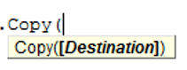
Using this method copies everything – values, formats, formulas and so on. If you want to copy individual items you can use the PasteSpecial property of range.
It works like this
Range("A1:B4").Copy
Range("F3").PasteSpecial Paste:=xlPasteValues
Range("F3").PasteSpecial Paste:=xlPasteFormats
Range("F3").PasteSpecial Paste:=xlPasteFormulas
The following table shows a full list of all the paste types
| Paste Type |
|---|
| xlPasteAll |
| xlPasteAllExceptBorders |
| xlPasteAllMergingConditionalFormats |
| xlPasteAllUsingSourceTheme |
| xlPasteColumnWidths |
| xlPasteComments |
| xlPasteFormats |
| xlPasteFormulas |
| xlPasteFormulasAndNumberFormats |
| xlPasteValidation |
| xlPasteValues |
| xlPasteValuesAndNumberFormats |
Reading a Range of Cells to an Array
You can also copy values by assigning the value of one range to another.
Range("A3:Z3").Value2 = Range("A1:Z1").Value2
The value of range in this example is considered to be a variant array. What this means is that you can easily read from a range of cells to an array. You can also write from an array to a range of cells. If you are not familiar with arrays you can check them out in this post.
The following code shows an example of using an array with a range:
' https://excelmacromastery.com/
Public Sub ReadToArray()

    ' Create dynamic array
    Dim StudentMarks() As Variant

    ' Read 26 values into array from the first row
    StudentMarks = Range("A1:Z1").Value2

    ' Do something with array here

    ' Write the 26 values to the third row
    Range("A3:Z3").Value2 = StudentMarks

End Sub
Keep in mind that the array created by the read is a 2 dimensional array. This is because a spreadsheet stores values in two dimensions i.e. rows and columns
Going through all the cells in a Range
Sometimes you may want to go through each cell one at a time to check value.
You can do this using a For Each loop shown in the following code
' https://excelmacromastery.com/
Public Sub TraversingCells()

    ' Go through each cells in the range
    Dim rg As Range
    For Each rg In Sheet1.Range("A1:A10,A20")
        ' Print address of cells that are negative
        If rg.Value < 0 Then
            Debug.Print rg.Address + " is negative."
        End If
    Next

End Sub
You can also go through consecutive Cells using the Cells property and a standard For loop.
The standard loop is more flexible about the order you use but it is slower than a For Each loop.
' https://excelmacromastery.com/
Public Sub TraverseCells()

    ' Go through cells from A1 to A10
    Dim i As Long
    For i = 1 To 10
        ' Print address of cells that are negative
        If Range("A" & i).Value < 0 Then
            Debug.Print Range("A" & i).Address + " is negative."
        End If
    Next

    ' Go through cells in reverse i.e. from A10 to A1
    For i = 10 To 1 Step -1
        ' Print address of cells that are negative
        If Range("A" & i) < 0 Then
            Debug.Print Range("A" & i).Address + " is negative."
        End If
    Next

End Sub
Formatting Cells
Sometimes you will need to format the cells the in spreadsheet. This is actually very straightforward. The following example shows you various formatting you can add to any range of cells
' https://excelmacromastery.com/
Public Sub FormattingCells()

    With Sheet1

        ' Format the font
        .Range("A1").Font.Bold = True
        .Range("A1").Font.Underline = True
        .Range("A1").Font.Color = rgbNavy

        ' Set the number format to 2 decimal places
        .Range("B2").NumberFormat = "0.00"
        ' Set the number format to a date
        .Range("C2").NumberFormat = "dd/mm/yyyy"
        ' Set the number format to general
        .Range("C3").NumberFormat = "General"
        ' Set the number format to text
        .Range("C4").NumberFormat = "Text"

        ' Set the fill color of the cell
        .Range("B3").Interior.Color = rgbSandyBrown

        ' Format the borders
        .Range("B4").Borders.LineStyle = xlDash
        .Range("B4").Borders.Color = rgbBlueViolet

    End With

End Sub
Main Points
The following is a summary of the main points
- Range returns a range of cells
- Cells returns one cells only
- You can read from one cell to another
- You can read from a range of cells to another range of cells.
- You can read values from cells to variables and vice versa.
- You can read values from ranges to arrays and vice versa
- You can use a For Each or For loop to run through every cell in a range.
- The properties Rows and Columns allow you to access a range of cells of these types
What’s Next?
Free VBA Tutorial If you are new to VBA or you want to sharpen your existing VBA skills then why not try out the The Ultimate VBA Tutorial.
Related Training: Get full access to the Excel VBA training webinars and all the tutorials.
(NOTE: Planning to build or manage a VBA Application? Learn how to build 10 Excel VBA applications from scratch.)
The VBA Range Object
The Excel Range Object is an object in Excel VBA that represents a cell, row, column, a selection of cells or a 3 dimensional range. The Excel Range is also a Worksheet property that returns a subset of its cells.
Worksheet Range
The Range is a Worksheet property which allows you to select any subset of cells, rows, columns etc.
Dim r as Range 'Declared Range variable

Set r = Range("A1") 'Range of A1 cell

Set r = Range("A1:B2") 'Square Range of 4 cells - A1,A2,B1,B2

Set r= Range(Range("A1"), Range ("B1")) 'Range of 2 cells A1 and B1

Range("A1:B2").Select 'Select the Cells A1:B2 in your Excel Worksheet

Range("A1:B2").Activate 'Activate the cells and show them on your screen (will switch to Worksheet and/or scroll to this range.
Select a cell or Range of cells using the Select method. It will be visibly marked in Excel:
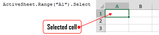
Working with Range variables
The Range is a separate object variable and can be declared as other variables. As the VBA Range is an object you need to use the Set statement:
Dim myRange as Range
'...
Set myRange = Range("A1") 'Need to use Set to define myRange
The Range object defaults to your ActiveWorksheet. So beware as depending on your ActiveWorksheet the Range object will return values local to your worksheet:
Range("A1").Select
'...is the same as...
ActiveSheet.Range("A1").Select
You might want to define the Worksheet reference by Range if you want your reference values from a specifc Worksheet:
Sheets("Sheet1").Range("A1").Select 'Will always select items from Worksheet named Sheet1
The ActiveWorkbook is not same to ThisWorkbook. Same goes for the ActiveSheet. This may reference a Worksheet from within a Workbook external to the Workbook in which the macro is executed as Active references simply the currently top-most worksheet. Read more here
Range properties
The Range object contains a variety of properties with the main one being it’s Value and an the second one being its Formula.
A Range Value is the evaluated property of a cell or a range of cells. For example a cell with the formula =10+20 has an evaluated value of 20.
A Range Formula is the formula provided in the cell or range of cells. For example a cell with a formula of =10+20 will have the same Formula property.
'Let us assume A1 contains the formula "=10+20"

Debug.Print Range("A1").Value 'Returns: 30

Debug.Print Range("A1").Formula 'Returns: =10+20
Other Range properties include:
Work in progress
Worksheet Cells
A Worksheet Cells property is similar to the Range property but allows you to obtain only a SINGLE CELL, based on its row and column index. Numbering starts at 1:

The Cells property is in fact a Range object not a separate data type.
Excel facilitates a Cells function that allows you to obtain a cell from within the ActiveSheet, current top-most worksheet.
Cells(2,2).Select 'Selects B2
'...is the same as...
ActiveSheet.Cells(2,2).Select 'Select B2
Cells are Ranges which means they are not a separate data type:
Dim myRange as Range
Set myRange = Cells(1,1) 'Cell A1
Range Rows and Columns
As we all know an Excel Worksheet is divided into Rows and Columns. The Excel VBA Range object allows you to select single or multiple rows as well as single or multiple columns. There are a couple of ways to obtain Worksheet rows in VBA:
Getting an entire row or column
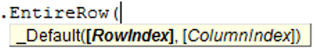
 To get and entire row of a specified Range you need to use the EntireRow property. Although, the function’s parameters suggest taking both a RowIndex and ColumnIndex it is enough just to provide the row number. Row indexing starts at 1.
 To get and entire column of a specified Range you need to use the EntireColumn property. Although, the function’s parameters suggest taking both a RowIndex and ColumnIndex it is enough just to provide the column number. Column indexing starts at 1.
Range("B2").EntireRows(1).Hidden = True 'Gets and hides the entire row 2

Range("B2").EntireColumns(1).Hidden = True 'Gets and hides the entire column 2
The three properties EntireRow/EntireColumn, Rows/Columns and Row/Column are often misunderstood so read through to understand the differences.
Get a row/column of a specified range
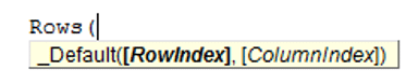 If you want to get a certain row within a Range simply use the Rows property of the Worksheet. Although, the function’s parameters suggest taking both a RowIndex and ColumnIndex it is enough just to provide the row number. Row indexing starts at 1.
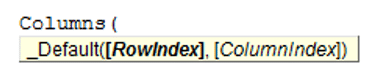 Similarly you can use the Columns function to obtain any single column within a Range. Although, the function’s parameters suggest taking both a RowIndex and ColumnIndex actually the first argument you provide will be the column index. Column indexing starts at 1.
Rows(1).Hidden = True 'Hides the first row in the ActiveSheet
'same as
ActiveSheet.Rows(1).Hidden = True

Columns(1).Hidden = True 'Hides the first column in the ActiveSheet
'same as
ActiveSheet.Columns(1).Hidden = True
To get a range of rows/columns you need to use the Range function like so:
Range(Rows(1), Rows(3)).Hidden = True 'Hides rows 1:3
'same as
Range("1:3").Hidden = True
'same as
ActiveSheet.Range("1:3").Hidden = True

Range(Columns(1), Columns(3)).Hidden = True 'Hides columns A:C
'same as
Range("A:C").Hidden = True
'same as
ActiveSheet.Range("A:C").Hidden = True
Get row/column of specified range
The above approach assumed you want to obtain only rows/columns from the ActiveSheet – the visible and top-most Worksheet. Usually however, you will want to obtain rows or columns of an existing Range. Similarly as with the Worksheet Range property, any Range facilitates the Rows and Columns property.
Dim myRange as Range
Set myRange = Range("A1:C3")

myRange.Rows.Hidden = True 'Hides rows 1:3
myRange.Columns.Hidden = True 'Hides columns A:C

Set myRange = Range("C10:F20")
myRange.Rows(2).Hidden = True 'Hides rows 11
myRange.Columns(3).Hidden = True 'Hides columns E
Getting a Ranges first row/column number
Aside from the Rows and Columns properties Ranges also facilitate a Row and Column property which provide you with the number of the Ranges first row and column.
Set myRange = Range("C10:F20")

'Get first row number
Debug.Print myRange.Row 'Result: 10
'Get first column number
Debug.Print myRange.Column 'Result: 3
Converting Column number to Excel Column
This is an often question that turns up – how to convert a column number to a string e.g. 100 to “CV”.
Function GetExcelColumn(columnNumber As Long)
    Dim div As Long, colName As String, modulo As Long
    div = columnNumber: colName = vbNullString

    Do While div > 0
        modulo = (div - 1) Mod 26
        colName = Chr(65 + modulo) & colName
        div = ((div - modulo) / 26)
    Loop

    GetExcelColumn = colName
End Function
Range Cut/Copy/Paste
Cutting and pasting rows is generally a bad practice which I heavily discourage as this is a practice that is moments can be heavily cpu-intensive and often is unaccounted for.
Copy function
 The Copy function works on a single cell, subset of cell or subset of rows/columns.
'Copy values and formatting from cell A1 to cell D1
Range("A1").Copy Range("D1")

'Copy 3x3 A1:C3 matrix to D1:F3 matrix - dimension must be same
Range("A1:C3").Copy Range("D1:F3")

'Copy rows 1:3 to rows 4:6
Range("A1:A3").EntireRow.Copy Range("A4")

'Copy columns A:C to columns D:F
Range("A1:C1").EntireColumn.Copy Range("D1")
The Copy function can also be executed without an argument. It then copies the Range to the Windows Clipboard for later Pasting.
Cut function
![]() The Cut function, similarly as the Copy function, cuts single cells, ranges of cells or rows/columns.
The Cut function, similarly as the Copy function, cuts single cells, ranges of cells or rows/columns.
'Cut A1 cell and paste it to D1
Range("A1").Cut Range("D1")

'Cut 3x3 A1:C3 matrix and paste it in D1:F3 matrix - dimension must be same
Range("A1:C3").Cut Range("D1:F3")

'Cut rows 1:3 and paste to rows 4:6
Range("A1:A3").EntireRow.Cut Range("A4")

'Cut columns A:C and paste to columns D:F
Range("A1:C1").EntireColumn.Cut Range("D1")
The Cut function can be executed without arguments. It will then cut the contents of the Range and copy it to the Windows Clipboard for pasting.
Cutting cells/rows/columns does not shift any remaining cells/rows/columns but simply leaves the cut out cells empty
PasteSpecial function
 The Range PasteSpecial function works only when preceded with either the Copy or Cut Range functions. It pastes the Range (or other data) within the Clipboard to the Range on which it was executed.
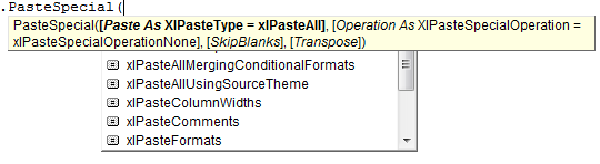
Syntax
The PasteSpecial function has the following syntax:
PasteSpecial( Paste, Operation, SkipBlanks, Transpose)
The PasteSpecial function can only be used in tandem with the Copy function (not Cut)
Parameters
Paste
The part of the Range which is to be pasted. This parameter can have the following values:
| Parameter | Constant | Description | |
|---|---|---|---|
| xlPasteSpecialOperationAdd | 2 | Copied data will be added with the value in the destination cell. | |
| xlPasteSpecialOperationDivide | 5 | Copied data will be divided with the value in the destination cell. | |
| xlPasteSpecialOperationMultiply | 4 | Copied data will be multiplied with the value in the destination cell. | |
| xlPasteSpecialOperationNone | -4142 | No calculation will be done in the paste operation. | |
| xlPasteSpecialOperationSubtract | 3 | Copied data will be subtracted with the value in the destination cell. |
Operation
The paste operation e.g. paste all, only formatting, only values, etc. This can have one of the following values:
| Name | Constant | Description |
|---|---|---|
| xlPasteAll | -4104 | Everything will be pasted. |
| xlPasteAllExceptBorders | 7 | Everything except borders will be pasted. |
| xlPasteAllMergingConditionalFormats | 14 | Everything will be pasted and conditional formats will be merged. |
| xlPasteAllUsingSourceTheme | 13 | Everything will be pasted using the source theme. |
| xlPasteColumnWidths | 8 | Copied column width is pasted. |
| xlPasteComments | -4144 | Comments are pasted. |
| xlPasteFormats | -4122 | Copied source format is pasted. |
| xlPasteFormulas | -4123 | Formulas are pasted. |
| xlPasteFormulasAndNumberFormats | 11 | Formulas and Number formats are pasted. |
| xlPasteValidation | 6 | Validations are pasted. |
| xlPasteValues | -4163 | Values are pasted. |
| xlPasteValuesAndNumberFormats | 12 | Values and Number formats are pasted. |
SkipBlanks
If True then blanks will not be pasted.
Transpose
Transpose the Range before paste (swap rows with columns).
PasteSpecial Examples
'Cut A1 cell and paste its values to D1
Range("A1").Copy
Range("D1").PasteSpecial
'Copy 3x3 A1:C3 matrix and add all the values to E1:G3 matrix (dimension must be same)
Range("A1:C3").Copy
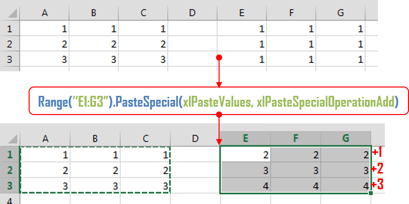
Range("E1:G3").PasteSpecial xlPasteValues, xlPasteSpecialOperationAdd
Below an example where the Excel Range A1:C3 values are copied an added to the E1:G3 Range. You can also multiply, divide and run other similar operations.
Paste
The Paste function allows you to paste data in the Clipboard to the actively selected Range. Cutting and Pasting can only be accomplished with the Paste function.
'Cut A1 cell and paste its values to D1
Range("A1").Cut
Range("D1").Select
ActiveSheet.Paste

'Cut 3x3 A1:C3 matrix and paste it in D1:F3 matrix - dimension must be same
Range("A1:C3").Cut
Range("D1:F3").Select
ActiveSheet.Paste

'Cut rows 1:3 and paste to rows 4:6
Range("A1:A3").EntireRow.Cut
Range("A4").Select
ActiveSheet.Paste

'Cut columns A:C and paste to columns D:F
Range("A1:C1").EntireColumn.Cut
Range("D1").Select
ActiveSheet.Paste
Range Clear/Delete
The Clear function
The Clear function clears the entire content and formatting from an Excel Range. It does not, however, shift (delete) the cleared cells.
Range("A1:C3").Clear
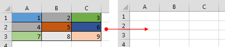
The Delete function
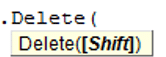 The Delete function deletes a Range of cells, removing them entirely from the Worksheet, and shifts the remaining Cells in a selected shift direction.
Although the manual Delete cell function provides 4 ways of shifting cells. The VBA Delete Shift values can only be either be xlShiftToLeft or xlShiftUp.
'If Shift omitted, Excel decides - shift up in this case
Range("B2").Delete

'Delete and Shift remaining cells left
Range("B2").Delete xlShiftToLeft

'Delete and Shift remaining cells up
Range("B2").Delete xlShiftTop

'Delete entire row 2 and shift up
Range("B2").EntireRow.Delete

'Delete entire column B and shift left
Range("B2").EntireRow.Delete
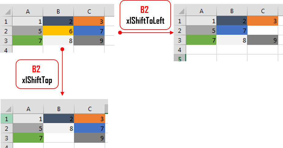
Traversing Ranges
Traversing cells is really useful when you want to run an operation on each cell within an Excel Range. Fortunately this is easily achieved in VBA using the For Each or For loops.
Dim cellRange As Range

For Each cellRange In Range("A1:C3")
  Debug.Print cellRange.Value
Next cellRange
Although this may not be obvious, beware of iterating/traversing the Excel Range using a simple For loop. For loops are not efficient on Ranges. Use a For Each loop as shown above. This is because Ranges resemble more Collections than Arrays. Read more on For vs For Each loops here
Traversing the UsedRange
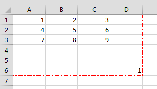 Every Worksheet has a UsedRange. This represents that smallest rectangle Range that contains all cells that have or had at some point values. In other words if the further out in the bottom, right-corner of the Worksheet there is a certain cell (e.g. E8) then the UsedRange will be as large as to include that cell starting at cell A1 (e.g. A1:E8). In Excel you can check the current UsedRange hitting CTRL+END. In VBA you get the UsedRange like this:
ActiveSheet.UsedRange
'same as
UsedRange
You can traverse through the UsedRange like this:
Dim cellRange As Range

For Each cellRange In UsedRange
  Debug.Print "Row: " & cellRange.Row & ", Column: " & cellRange.Column
Next cellRange
The UsedRange is a useful construct responsible often for bloated Excel Workbooks. Often delete unused Rows and Columns that are considered to be within the UsedRange can result in significantly reducing your file size. Read also more on the XSLB file format here
Range Addresses
The Excel Range Address property provides a string value representing the Address of the Range.
![]()
Syntax
Below the syntax of the Excel Range Address property:
Address( [RowAbsolute], [ColumnAbsolute], [ReferenceStyle], [External], [RelativeTo] )
Parameters
RowAbsolute
Optional. If True returns the row part of the reference address as an absolute reference. By default this is True.
$D$10:$G$100 'RowAbsolute is set to True
$D10:$G100 'RowAbsolute is set to False
ColumnAbsolute
Optional. If True returns the column part of the reference as an absolute reference. By default this is True.
$D$10:$G$100 'ColumnAbsolute is set to True
D$10:G$100 'ColumnAbsolute is set to False
ReferenceStyle
Optional. The reference style. The default value is xlA1. Possible values:
| Constant | Value | Description |
|---|---|---|
| xlA1 | 1 | Default. Use xlA1 to return an A1-style reference |
| xlR1C1 | -4150 | Use xlR1C1 to return an R1C1-style reference |
External
Optional. If True then property will return an external reference address, otherwise a local reference address will be returned. By default this is False.
$A$1 'Local
[Book1.xlsb]Sheet1!$A$1 'External
RelativeTo
Provided RowAbsolute and ColumnAbsolute are set to False, and the ReferenceStyle is set to xlR1C1, then you must include a starting point for the relative reference. This must be a Range variable to be set as the reference point.
Merged Ranges
![]() Merged cells are Ranges that consist of 2 or more adjacent cells. To Merge a collection of adjacent cells run Merge function on that Range.
Merged cells are Ranges that consist of 2 or more adjacent cells. To Merge a collection of adjacent cells run Merge function on that Range.
The Merge has only a single parameter – Across, a boolean which if True will merge cells in each row of the specified range as separate merged cells. Otherwise the whole Range will be merged. The default value is False.
Merge examples
To merge the entire Range:
'This will turn of any alerts warning that values may be lost
Application.DisplayAlerts = False

Range("B2:C3").Merge
This will result in the following:
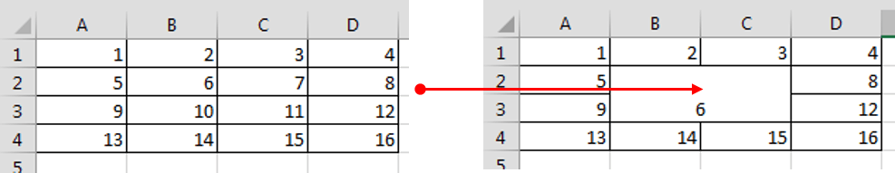
To merge just the rows set Across to True.
'This will turn of any alerts warning that values may be lost
Application.DisplayAlerts = False

Range("B2:C3").Merge True
This will result in the following:
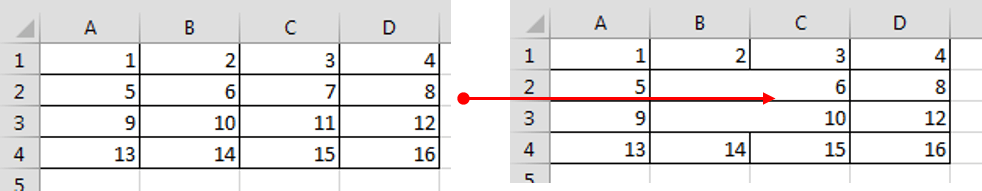
Remember that merged Ranges can only have a single value and formula. Hence, if you merge a group of cells with more than a single value/formula only the first value/formula will be set as the value/formula for your new merged Range
Checking if Range is merged
To check if a certain Range is merged simply use the Excel Range MergeCells property:
Range("B2:C3").Merge

Debug.Print Range("B2").MergeCells 'Result: True
The MergeArea
The MergeArea is a property of an Excel Range that represent the whole merge Range associated with the current Range. Say that $B$2:$C$3 is a merged Range – each cell within that Range (e.g. B2, C3..) will have the exact same MergedArea. See example below:
Range("B2:C3").Merge
Debug.Print Range("B2").MergeArea.Address 'Result: $B$2:$C$3
Named Ranges
Named Ranges are Ranges associated with a certain Name (string). In Excel you can find all your Named Ranges by going to Formulas->Name Manager. They are very useful when working on certain values that are used frequently through out your Workbook. Imagine that you are writing a Financial Analysis and want to use a common Discount Rate across all formulas. Just the address of the cell e.g. “A2”, won’t be self-explanatory. Why not use e.g. “DiscountRate” instead? Well you can do just that.
Creating a Named Range
Named Ranges can be created either within the scope of a Workbook or Worksheet:
Dim r as Range
'Within Workbook
Set r = ActiveWorkbook.Names.Add("NewName", Range("A1"))
'Within Worksheet
Set r = ActiveSheet.Names.Add("NewName", Range("A1"))
This gives you flexibility to use similar names across multiple Worksheets or use a single global name across the entire Workbook.
Listing all Named Ranges
You can list all Named Ranges using the Name Excel data type. Names are objects that represent a single NamedRange. See an example below of listing our two newly created NamedRanges:
Call ActiveWorkbook.Names.Add("NewName", Range("A1"))
Call ActiveSheet.Names.Add("NewName", Range("A1"))

Dim n As Name
For Each n In ActiveWorkbook.Names
  Debug.Print "Name: " & n.Name & ", Address: " & _
       n.RefersToRange.Address & ", Value: "; n.RefersToRange.Value
Next n

'Result:
'Name: Sheet1!NewName, Address: $A$1, Value:  1
'Name: NewName, Address: $A$1, Value:  1
SpecialCells
SpecialCells are a very useful Excel Range property, that allows you to select a subset of cells/Ranges within a certain Range.
Syntax
The SpecialCells property has the following syntax:
SpecialCells( Type, [Value] )
Parameters
Type
The type of cells to be returned. Possible values:
| Constant | Value | Description |
|---|---|---|
| xlCellTypeAllFormatConditions | -4172 | Cells of any format |
| xlCellTypeAllValidation | -4174 | Cells having validation criteria |
| xlCellTypeBlanks | 4 | Empty cells |
| xlCellTypeComments | -4144 | Cells containing notes |
| xlCellTypeConstants | 2 | Cells containing constants |
| xlCellTypeFormulas | -4123 | Cells containing formulas |
| xlCellTypeLastCell | 11 | The last cell in the used range |
| xlCellTypeSameFormatConditions | -4173 | Cells having the same format |
| xlCellTypeSameValidation | -4175 | Cells having the same validation criteria |
| xlCellTypeVisible | 12 | All visible cells |
Value
If Type is equal to xlCellTypeConstants or xlCellTypeFormulas this determines the types of cells to return e.g. with errors.
| Constant | Value |
|---|---|
| xlErrors | 16 |
| xlLogical | 4 |
| xlNumbers | 1 |
| xlTextValues | 2 |
SpecialCells examples
Get Excel Range with Constants
This will return only cells with constant cells within the Range C1:C3:
For Each r In Range("A1:C3").SpecialCells(xlCellTypeConstants)
  Debug.Print r.Value
Next r
Search for Excel Range with Errors
For Each r In ActiveSheet.UsedRange.SpecialCells(xlCellTypeFormulas, xlErrors)
  Debug.Print r.Address
Next r
Свойства
Cвойство Range
Свойство Range возвращает объект Range, определяемый аргументами. Используются два разных способа записи свойства Range.
Первый способ object.Range(Cell1)
Второй способ object.Range(Cell1 [,Cell2])
- object — ссылка на объект, например, на рабочий лист или на интервал ячеек. Ссылка необязательна. По умолчанию используется активный лист;
- Cell1, Cell2 — аргументы для задания интервала ячеек. Cell1 — указание обязательно при обоих способах записи свойства Range.
Первый способ
Аргумент Cell1 задает интервал ячеек произвольного размера.
Важно
- Могут использоваться имена, определенные в таблице, или координаты ячеек, столбцов, строк или интервалов.
- Координаты задаются в стиле A1.
- Координаты и имена заключаются в кавычки.
- При задании интервалов координаты левого верхнего угла и правого нижнего угла интервала разделяются двоеточием.
- Для задания несмежных интервалов используется запятая.
- Для задания пересечения интервалов используется пробел.
| Запись | Возвращаемый объект |
|---|---|
| ActiveSheet.Range(«A1:A10«) | интервал ячеек A1:A10 на активном листе |
| Range(«A:B») | столбцы A:B |
| Range(«налог») | интервал с именем налог |
| Range(«1:3») | строки с первой по третью |
| Range(«A1:C2, B10:D24″) | объединение двух несмежных интервалов A1:C2 и B10:D24 |
| Range(«A1:C10 B10:D24») | пересечение двух интервалов A1:C10 и B10:D24, т.е. интервал B10:C10 |
Второй способ
Аргументы задают координаты интервала:
- Cell1 — единственная ячейка (строка или столбец), задающая левый верхний угол интервала;
- Cell2 — единственная ячейка (строка или столбец), задающая правый нижний угол интервала. Необязательный аргумент.
Допустимо задание аргументов переменными, выражениями, свойствами или методами, представляющими объект Range — одну ячейку, одну строку или один столбец рабочего листа.
| Запись | Возвращаемый объект |
|---|---|
| Range(«A5″,»D18») | интервал A5:D18 |
| Range(Columns(1), Columns(5)) | интервал, содержащий первые пять столбцов рабочего листа |
ЗАПОМНИТЕ
- Если свойство Range применяется к объекту Range, то ссылка на интервал ячеек считается относительной и возвращается смещенный объект Range.
Например, если выделен интервал C1:D5, то запись Selection.Range(«B2») возвратит ячейку D2.
Свойство Cells
Свойство Cells возвращает единственную ячейку рабочего листа, которая находится на пересечении строки и столбца, задаваемых целыми числами.
Синтаксис object.Cells (RowIndex,ColumnIndex)
- object — ссылка на объект. Ссылка необязательна. По умолчанию используется активный лист;
- RowIndex — индекс строки;
- ColumnIndex — индекс столбца.
ЗАМЕЧАНИЯ
- В свойстве Cells индекс строки является первым аргументом, а индекс столбца — вторым аргументом, тогда как при задании адреса ячейки в стиле A1 сначала указывается столбец, а затем строка.
- Понятие «индекс» ( Index, ColumnIndex, RowIndex ) всегда подразумевает целое число, целочисленную переменную или выражение, результат вычисления которого есть целое число или может быть преобразован в целое число.
| Запись | Комментарий | Возвращаемый объект |
|---|---|---|
| ActiveSheet.Cells | Свойство Cells без аргументов | все ячейки активного рабочего листа |
| Range(«C5:C10»).Cells(1,1) | Свойство Cells применяется к объекту Range (относительная ссылка) | ячейка C5 |
| Range(Cells(7,3),Cells(10,4)) | Свойство Cells используется в качестве аргументов свойства Range | интервал ячеек C7:D10 |
Свойство Offset
Свойство Offset позволяет задавать ячейки или интервалы при помощи числа строк и колонок, которые отделяют нужную ячейку от исходной ячейки, т.е. указывая смещение относительно выбранной ячейки. Например, Range(«A5»).Offset(-2,1) возвращает ячейку B3.
Синтаксис object.Offset([RowOffset][,ColumnOffset])
- object — ссылка на объект Range. Ссылка обязательна и определяет объект, относительно которого задается смещение;
- RowOffset — смещение строки искомой ячейки относительно исходной ячейки;
- ColumnOffset — смещение столбца искомой ячейки относительно исходной ячейки.
Необязательные аргументы RowOffset и ColumnOffset — числовые выражения. Если какой-то аргумент не задан, то соответствующее смещение равно нулю.
Например, если выделен интервал C1:D5, то запись Selection.Offset(2,1).Select выделяет интервал D3:E7.
Метод Union и свойство Areas
Метод Union используется для объединения двух и более объектов Range, заданных ссылками на непересекающиеся интервалы, в один объект Range.
Синтаксис Object.Union (arg1,arg2,…)
- object — всегда объект Application. Ссылка необязательна;
- arg1,arg2 — интервалы ячеек. Количество аргументов произвольно. Обязательно наличие хотя бы двух аргументов.
Например, оператор Union(Range(«A1:C5»),Range(«B10:D12»)).Select выделяет несмежные интервалы A1:C5 и B10:D12.
Свойство Areas выполняет обратное действие, разделяя объединенные интервалы на несколько объектов Range.
Синтаксис Object.Areas(index)
- object — ссылка на объект Range, состоящий из нескольких интервалов;
- index — номер интервала в объекте. Аргумент необязателен.
| Оператор | Комментарий | Результат |
|---|---|---|
| p=Union (Range(«A1:C5»), Range(«B10:D12»)).Areas(2).Count | Если аргумент задан, то свойство Areas возвращает интервал — объект Range, определенный индексом интервала | равен девяти, так как во втором интервале ровно 9 ячеек |
| p=Union(Range(«A1:C5»), Range(«B10:D12»)).Areas.Count | Cвойство Areas без аргументов рассматривает каждый из несмежных интервалов как элемент коллекции объектов Range | равен двум, так как объект, определенный методом Union, состоит из двух областей — коллекции из двух элементов |
| p=Range(«B10:D12»).Areas.Count | равен единице, так как объект Range представляет один элемент коллекции |
Свойства Column и Row (R/O Integer)
Свойства возвращают целое число, показывающее индекс первого столбца или первой строки соответственно для заданного объекта. Синтаксис свойств
- object — обязательная ссылка на объект Range.
Например, запись Range(«C5»).Column возвращает число 3, а запись Range(«C5»).Row возвращает число 5.
Свойства Columns и Rows
Свойство Columns (не путайте со свойством Column!) возвращает объект Range, представляющий колонку или коллекцию колонок в объекте, к которому это свойство было применено.
Синтаксис Object.Columns(index)
- object — ссылка на объект. Указание необязательно, по умолчанию используется активный рабочий лист;
- index — индекс колонки в объекте.
Например, запись Columns(1) возвращает колонку A активного рабочего листа, а запись Range(«C1:D5»).Columns(1) возвращает колонку C заданного интервала, а именно, ячейки C1:C5.
Важно
- Если не указан индекс колонки, то возвращаются все колонки объекта в виде объекта Range.
- Индекс колонки можно указывать числом или буквой, при этом буква заключается в кавычки. Ссылки Columns(2) и Columns(«B») указывают на одну и ту же колонку B.
Свойство Rows (не путайте со свойством Row!) возвращает объект Range, представляющий строку или коллекцию строк в объекте, к которому это свойство было применено.
Синтаксис Object.Rows(index)
- object — ссылка на объект. Указание необязательно, по умолчанию используется активный рабочий лист;
- index — индекс строки в объекте.
Важно
- Если не указан номер строки, то возвращаются все строки объекта в виде объекта Range.
Например, оператор nr=Selection.Rows(Selection.Rows.Count).Row позволяет получить номер последней строки в выделенном интервале ячеек.
Свойство CurrentRegion
Свойство CurrentRegion определяет объект Range, который соответствует интервалу ячеек, включающему заданную ячейку.
Пример
В процедуре сравниваются значения первой ячейки первой строки и первой ячейки каждой следующей строки заполненного данными интервала, включающего первую ячейку. Если значения совпадают, то очередная строка удаляется.
Предполагается, что данные начинаются с ячейки A1 и занимают несколько строк и столбцов, при этом расположены не плотно, т.е. внутри интервала с данными могут находиться пустые строки или пустые столбцы. Анализируются только строки заполненного данными интервала ячеек вокруг ячейки A1, не содержащего пустых строк и столбцов.
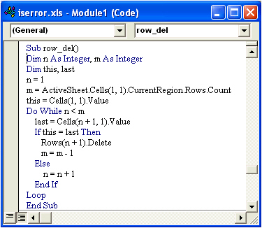
Рис.
8.9.
Пример работы со свойством CurrentRegion
| Свойства | Примеры и комментарии |
|---|---|
| ColumnWidth (R/W Variant) | Возвращает или изменяет ширину колонки в единицах, эквивалентных одному символу в стиле Обычный ( Normal ). Шрифт стиля по умолчанию Arial Cyr и размер шрифта 10.
Range(«A1»).ColumnWidth=15 устанавливает ширину колонки A в 15 символов |
| Width (R/O Variant) | Возвращает ширину интервала ячеек в пунктах.
Range(«A1»).Width возвращает значение 93.75, если ширина колонки 15 символов, шрифт Times New Roman, размер шрифта 12 пунктов (72 пункта равны 1 дюйму или приблизительно 2,54 см). Debug.Print Range(«A1:C3»).ColumnWidth распечатает значение 8.43, а оператор Debug.Print Range(«A1:C3»).Width распечатает значение 144, если для колонок установлена стандартная ширина, шрифт Arial Cyr и размер шрифта 10 |
| RowHeight (R/W Variant) | Возвращает или изменяет высоту строк интервала в пунктах.
ActiveCell.RowHeight = 14 устанавливает высоту строки, в которой находится активная ячейка, в 14 пунктов |
| Height (R/O Variant) | Возвращает суммарную высоту интервала строк, зависящую от названия и размера шрифта. Если шрифт Arial Cyr и размер шрифта 10, то Debug.Print Range(«A1»).Height распечатает 12,75 и Debug.Print Range(«A1:C3»).Height распечатает 38,25 |
| WrapText (R/W Boolean) |
Range(«A1»).WrapText=True
Значение True разбивает текст ячейки на несколько строк, если ширина столбца недостаточна для размещения текста целиком |
Замечание
- Свойства Width и Height имеют статус Read-Only для объектов Range, но для других объектов, например, для объекта Window, они имеют статус Read-Write.
Методы
Методы Select и Activate
Метод Select выделяет интервал ячеек.
Синтаксис object.Select(Replace)
- object — выделяемый объект типа Range. Ссылка на объект обязательна;
- Replace — для расширения выделения аргумент устанавливается в False. Если аргумент не задан или принимает значение True, то вместо старой области выделения создается новая область выделения. Необязательный параметр.
Метод Activate активизирует единственную ячейку.
Синтаксис object.Activate
- object — активизируемая ячейка. Ссылка на объект обязательна.
| Оператор | Активная ячейка |
|---|---|
| Range(«C7:E9»).Select | C7 |
| Range(«C7:E9»).Offset(1,1).Activate | D8 |
| Range(«C7:E9»).Activate | C7 |
| Range(«C7:E9»).Cells(2,1).Activate | C8 |
ЗАМЕЧАНИЯ
- Активная ячейка выделяется фоном среди всех выделенных ячеек.
- Метод Select выделяет интервал ячеек, тогда как метод Activate активизирует только одну ячейку.
- При использовании метода Select первая ячейка интервала становится активной.
- Если выделена только одна ячейка, то она является активной и свойства ActiveCell и Selection возвращают одну и ту же ячейку (объект Range ).
Метод Clear
Очищает интервал ячеек, изменяя, таким образом, свойство Value каждой ячейки интервала.
Пример
Процедура очищает интервал ячеек или заполняет его единицами в зависимости от значений ячеек. Дополнительно изменяется шрифт и размер шрифта.
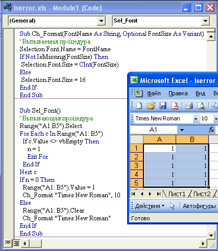
Рис.
8.10.
Пример применения метода Clear
Название шрифта является обязательным параметром вызываемой процедуры, а размер шрифта — необязательным параметром. Если он не задан, то размер шрифта принудительно меняется на 16.
Вызывающая процедура проверяет, является ли интервал ячеек A1:B5 пустым. Если это не так, то интервал очищается и размер шрифта устанавливается в 16. Если же интервал ячеек пуст, то все ячейки интервала заполняются единицами и размер шрифта интервала ячеек равен 10.
В обоих случаях шрифт ячеек интервала A1:B5 устанавливается в Times New Roman.
Цветовое оформление объекта Range
Свойство ColorIndex
Свойство ColorIndex заливки (заливка — это объект Interior, который является вложенным для объекта Range ) рассматривает цвет как номер в палитре цветов рабочей книги. Всего в палитре 56 цветов.
Пример
В ячейках, начиная с активной, отображается палитра цветов рабочей книги.
Переменные c и r содержат, соответственно, индекс столбца и индекс строки активной ячейки.
Прямоугольный интервал из 56 ячеек (7 строк и 8 столбцов, начиная с активной ячейки) для отображения палитры задается переменной obj_range, содержащей ссылку на объект Range.
Свойство Pattern (образец заливки) задается константой xlSolid, позволяющей установить заливку активных ячеек.
Свойство Color
Свойство относится к объектам Border, Font или Interior (вложенные объекты для объекта Range ) и устанавливает цвет объекта в формате RGB. Свойство можно задать, используя функцию RGB, которая возвращает цвет в виде числа типа Long. Аргументы функции Red, Green, Blue определяют насыщенность соответствующей компоненты в устанавливаемом цвете и изменяются от 0 до 255.
Например, оператор ActiveCell.Interior.Color=RGB(255, 0, 0) устанавливает красную заливку активной ячейки.
Замечание
- Не путайте свойство Color со свойством Colors! Последнее является свойством объекта Workbook и использует палитру цветов рабочей книги как массив значений цветов, например, оператор ActiveWorkbook.Colors(51) = RGB(255,0,0) меняет 51 цвет палитры активной рабочей книги на красный.
Чтобы использовать серый цвет разной интенсивности, установите равные аргументы функции RGB, например, выражение RGB(196,196,196) устанавливает 25% серую заливку. Чем больше значения аргументов, тем ближе серый цвет к белому.