
All About The Pivot Tables!
Pivot Tables and VBA can be a little tricky initially. Hopefully this guide will serve as a good resource as you try to automate those extremely powerful Pivot Tables in your Excel spreadsheets. Enjoy!
Create A Pivot Table
Sub CreatePivotTable()
‘PURPOSE: Creates a brand new Pivot table on a new worksheet from data in the ActiveSheet
‘Source: www.TheSpreadsheetGuru.com
Dim sht As Worksheet
Dim pvtCache As PivotCache
Dim pvt As PivotTable
Dim StartPvt As String
Dim SrcData As String
‘Determine the data range you want to pivot
SrcData = ActiveSheet.Name & «!» & Range(«A1:R100»).Address(ReferenceStyle:=xlR1C1)
‘Create a new worksheet
Set sht = Sheets.Add
‘Where do you want Pivot Table to start?
StartPvt = sht.Name & «!» & sht.Range(«A3»).Address(ReferenceStyle:=xlR1C1)
‘Create Pivot Cache from Source Data
Set pvtCache = ActiveWorkbook.PivotCaches.Create( _
SourceType:=xlDatabase, _
SourceData:=SrcData)
‘Create Pivot table from Pivot Cache
Set pvt = pvtCache.CreatePivotTable( _
TableDestination:=StartPvt, _
TableName:=»PivotTable1″)
End Sub
Delete A Specific Pivot Table
Sub DeletePivotTable()
‘PURPOSE: How to delete a specifc Pivot Table
‘SOURCE: www.TheSpreadsheetGuru.com
‘Delete Pivot Table By Name
ActiveSheet.PivotTables(«PivotTable1»).TableRange2.Clear
End Sub
Delete All Pivot Tables
Sub DeleteAllPivotTables()
‘PURPOSE: Delete all Pivot Tables in your Workbook
‘SOURCE: www.TheSpreadsheetGuru.com
Dim sht As Worksheet
Dim pvt As PivotTable
‘Loop Through Each Pivot Table In Currently Viewed Workbook
For Each sht In ActiveWorkbook.Worksheets
For Each pvt In sht.PivotTables
pvt.TableRange2.Clear
Next pvt
Next sht
End Sub
Add Pivot Fields
Sub Adding_PivotFields()
‘PURPOSE: Show how to add various Pivot Fields to Pivot Table
‘SOURCE: www.TheSpreadsheetGuru.com
Dim pvt As PivotTable
Set pvt = ActiveSheet.PivotTables(«PivotTable1»)
‘Add item to the Report Filter
pvt.PivotFields(«Year»).Orientation = xlPageField
‘Add item to the Column Labels
pvt.PivotFields(«Month»).Orientation = xlColumnField
‘Add item to the Row Labels
pvt.PivotFields(«Account»).Orientation = xlRowField
‘Position Item in list
pvt.PivotFields(«Year»).Position = 1
‘Format Pivot Field
pvt.PivotFields(«Year»).NumberFormat = «#,##0»
‘Turn on Automatic updates/calculations —like screenupdating to speed up code
pvt.ManualUpdate = False
End Sub
Add Calculated Pivot Fields
Sub AddCalculatedField()
‘PURPOSE: Add a calculated field to a pivot table
‘SOURCE: www.TheSpreadsheetGuru.com
Dim pvt As PivotTable
Dim pf As PivotField
‘Set Variable to Desired Pivot Table
Set pvt = ActiveSheet.PivotTables(«PivotTable1»)
‘Set Variable Equal to Desired Calculated Pivot Field
For Each pf In pvt.PivotFields
If pf.SourceName = «Inflation» Then Exit For
Next
‘Add Calculated Field to Pivot Table
pvt.AddDataField pf
End Sub
Add A Values Field
Sub AddValuesField()
‘PURPOSE: Add A Values Field to a Pivot Table
‘SOURCE: www.TheSpreadsheetGuru.com
Dim pvt As PivotTable
Dim pf As String
Dim pf_Name As String
pf = «Salaries»
pf_Name = «Sum of Salaries»
Set pvt = ActiveSheet.PivotTables(«PivotTable1»)
pvt.AddDataField pvt.PivotFields(«Salaries»), pf_Name, xlSum
End Sub
Remove Pivot Fields
Sub RemovePivotField()
‘PURPOSE: Remove a field from a Pivot Table
‘SOURCE: www.TheSpreadsheetGuru.com
‘Removing Filter, Columns, Rows
ActiveSheet.PivotTables(«PivotTable1»).PivotFields(«Year»).Orientation = xlHidden
‘Removing Values
ActiveSheet.PivotTables(«PivotTable1»).PivotFields(«Sum of Salaries»).Orientation = xlHidden
End Sub
Remove Calculated Pivot Fields
Sub RemoveCalculatedField()
‘PURPOSE: Remove a calculated field from a pivot table
‘SOURCE: www.TheSpreadsheetGuru.com
Dim pvt As PivotTable
Dim pf As PivotField
Dim pi As PivotItem
‘Set Variable to Desired Pivot Table
Set pvt = ActiveSheet.PivotTables(«PivotTable1»)
‘Set Variable Equal to Desired Calculated Data Field
For Each pf In pvt.DataFields
If pf.SourceName = «Inflation» Then Exit For
Next
‘Hide/Remove the Calculated Field
pf.DataRange.Cells(1, 1).PivotItem.Visible = False
End Sub
Report Filter On A Single Item
Sub ReportFiltering_Single()
‘PURPOSE: Filter on a single item with the Report Filter field
‘SOURCE: www.TheSpreadsheetGuru.com
Dim pf As PivotField
Set pf = ActiveSheet.PivotTables(«PivotTable2»).PivotFields(«Fiscal_Year»)
‘Clear Out Any Previous Filtering
pf.ClearAllFilters
‘Filter on 2014 items
pf.CurrentPage = «2014»
End Sub
Report Filter On Multiple Items
Sub ReportFiltering_Multiple()
‘PURPOSE: Filter on multiple items with the Report Filter field
‘SOURCE: www.TheSpreadsheetGuru.com
Dim pf As PivotField
Set pf = ActiveSheet.PivotTables(«PivotTable2»).PivotFields(«Variance_Level_1»)
‘Clear Out Any Previous Filtering
pf.ClearAllFilters
‘Enable filtering on multiple items
pf.EnableMultiplePageItems = True
‘Must turn off items you do not want showing
pf.PivotItems(«Jan»).Visible = False
pf.PivotItems(«Feb»).Visible = False
pf.PivotItems(«Mar»).Visible = False
End Sub
Clear Report Filter
Sub ClearReportFiltering()
‘PURPOSE: How to clear the Report Filter field
‘SOURCE: www.TheSpreadsheetGuru.com
Dim pf As PivotField
Set pf = ActiveSheet.PivotTables(«PivotTable2»).PivotFields(«Fiscal_Year»)
‘Option 1: Clear Out Any Previous Filtering
pf.ClearAllFilters
‘Option 2: Show All (remove filtering)
pf.CurrentPage = «(All)»
End Sub
Refresh Pivot Table(s)
Sub RefreshingPivotTables()
‘PURPOSE: Shows various ways to refresh Pivot Table Data
‘SOURCE: www.TheSpreadsheetGuru.com
‘Refresh A Single Pivot Table
ActiveSheet.PivotTables(«PivotTable1»).PivotCache.Refresh
‘Refresh All Pivot Tables
ActiveWorkbook.RefreshAll
End Sub
Change Pivot Table Data Source Range
Sub ChangePivotDataSourceRange()
‘PURPOSE: Change the range a Pivot Table pulls from
‘SOURCE: www.TheSpreadsheetGuru.com
Dim sht As Worksheet
Dim SrcData As String
Dim pvtCache As PivotCache
‘Determine the data range you want to pivot
Set sht = ThisWorkbook.Worksheets(«Sheet1»)
SrcData = sht.Name & «!» & Range(«A1:R100»).Address(ReferenceStyle:=xlR1C1)
‘Create New Pivot Cache from Source Data
Set pvtCache = ActiveWorkbook.PivotCaches.Create( _
SourceType:=xlDatabase, _
SourceData:=SrcData)
‘Change which Pivot Cache the Pivot Table is referring to
ActiveSheet.PivotTables(«PivotTable1»).ChangePivotCache (pvtCache)
End Sub
Grand Totals
Sub PivotGrandTotals()
‘PURPOSE: Show setup for various Pivot Table Grand Total options
‘SOURCE: www.TheSpreadsheetGuru.com
Dim pvt As PivotTable
Set pvt = ActiveSheet.PivotTables(«PivotTable1»)
‘Off for Rows and Columns
pvt.ColumnGrand = False
pvt.RowGrand = False
‘On for Rows and Columns
pvt.ColumnGrand = True
pvt.RowGrand = True
‘On for Rows only
pvt.ColumnGrand = False
pvt.RowGrand = True
‘On for Columns Only
pvt.ColumnGrand = True
pvt.RowGrand = False
End Sub
Report Layout
Sub PivotReportLayout()
‘PURPOSE: Show setup for various Pivot Table Report Layout options
‘SOURCE: www.TheSpreadsheetGuru.com
Dim pvt As PivotTable
Set pvt = ActiveSheet.PivotTables(«PivotTable1»)
‘Show in Compact Form
pvt.RowAxisLayout xlCompactRow
‘Show in Outline Form
pvt.RowAxisLayout xlOutlineRow
‘Show in Tabular Form
pvt.RowAxisLayout xlTabularRow
End Sub
Formatting A Pivot Table’s Data
Sub PivotTable_DataFormatting()
‘PURPOSE: Various ways to format a Pivot Table’s data
‘SOURCE: www.TheSpreadsheetGuru.com
Dim pvt As PivotTable
Set pvt = ActiveSheet.PivotTables(«PivotTable1»)
‘Change Data’s Number Format
pvt.DataBodyRange.NumberFormat = «#,##0;(#,##0)»
‘Change Data’s Fill Color
pvt.DataBodyRange.Interior.Color = RGB(0, 0, 0)
‘Change Data’s Font Type
pvt.DataBodyRange.Font.FontStyle = «Arial»
End Sub
Formatting A Pivot Field’s Data
Sub PivotField_DataFormatting()
‘PURPOSE: Various ways to format a Pivot Field’s data
‘SOURCE: www.TheSpreadsheetGuru.com
Dim pf As PivotField
Set pf = ActiveSheet.PivotTables(«PivotTable1»).PivotFields(«Months»)
‘Change Data’s Number Format
pf.DataRange.NumberFormat = «#,##0;(#,##0)»
‘Change Data’s Fill Color
pf.DataRange.Interior.Color = RGB(219, 229, 241)
‘Change Data’s Font Type
pf.DataRange.Font.FontStyle = «Arial»
End Sub
Expand/Collapse Entire Field Detail
Sub PivotField_ExpandCollapse()
‘PURPOSE: Shows how to Expand or Collapse the detail of a Pivot Field
‘SOURCE: www.TheSpreadsheetGuru.com
Dim pf As PivotField
Set pf = ActiveSheet.PivotTables(«PivotTable1»).PivotFields(«Month»)
‘Collapse Pivot Field
pf.ShowDetail = False
‘Expand Pivot Field
pf.ShowDetail = True
End Sub
Any Other Functionalities You Would Like To See?
I believe I was able to cover all the main pivot table VBA functionalities in this article, but there is so much you can do with pivot tables! Leave a comment below if you would like to see something else covered in this guide.
About The Author
Hey there! I’m Chris and I run TheSpreadsheetGuru website in my spare time. By day, I’m actually a finance professional who relies on Microsoft Excel quite heavily in the corporate world. I love taking the things I learn in the “real world” and sharing them with everyone here on this site so that you too can become a spreadsheet guru at your company.
Through my years in the corporate world, I’ve been able to pick up on opportunities to make working with Excel better and have built a variety of Excel add-ins, from inserting tickmark symbols to automating copy/pasting from Excel to PowerPoint. If you’d like to keep up to date with the latest Excel news and directly get emailed the most meaningful Excel tips I’ve learned over the years, you can sign up for my free newsletters. I hope I was able to provide you with some value today and hope to see you back here soon!
— Chris
Founder, TheSpreadsheetGuru.com
In this Article
- Using GetPivotData to Obtain a Value
- Creating a Pivot Table on a Sheet
- Creating a Pivot Table on a New Sheet
- Adding Fields to the Pivot Table
- Changing the Report Layout of the Pivot Table
- Deleting a Pivot Table
- Format all the Pivot Tables in a Workbook
- Removing Fields of a Pivot Table
- Creating a Filter
- Refreshing Your Pivot Table
This tutorial will demonstrate how to work with Pivot Tables using VBA.
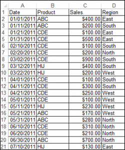
Pivot Tables are data summarization tools that you can use to draw key insights and summaries from your data. Let’s look at an example: we have a source data set in cells A1:D21 containing the details of products sold, shown below:
Using GetPivotData to Obtain a Value
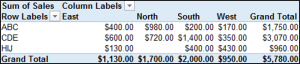
Assume you have a PivotTable called PivotTable1 with Sales in the Values/Data Field, Product as the Rows field and Region as the Columns field. You can use the PivotTable.GetPivotData method to return values from Pivot Tables.
The following code will return $1,130.00 (the total sales for the East Region) from the PivotTable:
MsgBox ActiveCell.PivotTable.GetPivotData("Sales", "Region", "East")
In this case, Sales is the “DataField”, “Field1” is the Region and “Item1” is East.
The following code will return $980 (the total sales for Product ABC in the North Region) from the Pivot Table:
MsgBox ActiveCell.PivotTable.GetPivotData("Sales", "Product", "ABC", "Region", "North")In this case, Sales is the “DataField”, “Field1” is Product, “Item1” is ABC, “Field2” is Region and “Item2” is North.
You can also include more than 2 fields.
The syntax for GetPivotData is:
GetPivotData (DataField, Field1, Item1, Field2, Item2…) where:
| Parameter | Description |
|---|---|
| Datafield | Data field such as sales, quantity etc. that contains numbers. |
| Field 1 | Name of a column or row field in the table. |
| Item 1 | Name of an item in Field 1 (Optional). |
| Field 2 | Name of a column or row field in the table (Optional). |
| Item 2 | Name of an item in Field 2 (Optional). |
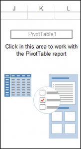
Creating a Pivot Table on a Sheet
In order to create a Pivot Table based on the data range above, on cell J2 on Sheet1 of the Active workbook, we would use the following code:
Worksheets("Sheet1").Cells(1, 1).Select

ActiveWorkbook.PivotCaches.Create(SourceType:=xlDatabase, SourceData:= _

 "Sheet1!R1C1:R21C4", Version:=xlPivotTableVersion15).CreatePivotTable _

  TableDestination:="Sheet1!R2C10", TableName:="PivotTable1", DefaultVersion _

  :=xlPivotTableVersion15

  Sheets("Sheet1").Select
The result is:
Creating a Pivot Table on a New Sheet
In order to create a Pivot Table based on the data range above, on a new sheet, of the active workbook, we would use the following code:
Worksheets("Sheet1").Cells(1, 1).Select

Sheets.Add

    ActiveWorkbook.PivotCaches.Create(SourceType:=xlDatabase, SourceData:= _

 "Sheet1!R1C1:R21C4", Version:=xlPivotTableVersion15).CreatePivotTable _

  TableDestination:="Sheet2!R3C1", TableName:="PivotTable1", DefaultVersion _

  :=xlPivotTableVersion15

  Sheets("Sheet2").Select
Adding Fields to the Pivot Table
You can add fields to the newly created Pivot Table called PivotTable1 based on the data range above. Note: The sheet containing your Pivot Table, needs to be the Active Sheet.
To add Product to the Rows Field, you would use the following code:
ActiveSheet.PivotTables("PivotTable1").PivotFields("Product").Orientation = xlRowField

ActiveSheet.PivotTables("PivotTable1").PivotFields("Product").Position = 1
To add Region to the Columns Field, you would use the following code:
ActiveSheet.PivotTables("PivotTable1").PivotFields("Region").Orientation = xlColumnField

ActiveSheet.PivotTables("PivotTable1").PivotFields("Region").Position = 1
To add Sales to the Values Section with the currency number format, you would use the following code:
ActiveSheet.PivotTables("PivotTable1").AddDataField ActiveSheet.PivotTables( _

        "PivotTable1").PivotFields("Sales"), "Sum of Sales", xlSum

    With ActiveSheet.PivotTables("PivotTable1").PivotFields("Sum of Sales")

        .NumberFormat = "$#,##0.00"

End With
The result is:
Changing the Report Layout of the Pivot Table
You can change the Report Layout of your Pivot Table. The following code will change the Report Layout of your Pivot Table to Tabular Form:
ActiveSheet.PivotTables("PivotTable1").TableStyle2 = "PivotStyleLight18"Deleting a Pivot Table
You can delete a Pivot Table using VBA. The following code will delete the Pivot Table called PivotTable1 on the Active Sheet:
ActiveSheet.PivotTables("PivotTable1").PivotSelect "", xlDataAndLabel, True
Selection.ClearContents
VBA Coding Made Easy
Stop searching for VBA code online. Learn more about AutoMacro — A VBA Code Builder that allows beginners to code procedures from scratch with minimal coding knowledge and with many time-saving features for all users!

Learn More
Format all the Pivot Tables in a Workbook
You can format all the Pivot Tables in a Workbook using VBA. The following code uses a loop structure in order to loop through all the sheets of a workbook, and formats all the Pivot Tables in the workbook:
Sub FormattingAllThePivotTablesInAWorkbook()
Dim wks As Worksheet
Dim wb As Workbook
Set wb = ActiveWorkbook
Dim pt As PivotTable

For Each wks In wb.Sheets
For Each pt In wks.PivotTables
pt.TableStyle2 = "PivotStyleLight15"
Next pt
Next wks

End Sub
To learn more about how to use Loops in VBA click here.
Removing Fields of a Pivot Table
You can remove fields in a Pivot Table using VBA. The following code will remove the Product field in the Rows section from a Pivot Table named PivotTable1 in the Active Sheet:
ActiveSheet.PivotTables("PivotTable1").PivotFields("Product").Orientation = _
xlHidden
Creating a Filter
A Pivot Table called PivotTable1 has been created with Product in the Rows section, and Sales in the Values Section. You can also create a Filter for your Pivot Table using VBA. The following code will create a filter based on Region in the Filters section:
ActiveSheet.PivotTables("PivotTable1").PivotFields("Region").Orientation = xlPageField

ActiveSheet.PivotTables("PivotTable1").PivotFields("Region").Position = 1
To filter your Pivot Table based on a Single Report Item in this case the East region, you would use the following code:
ActiveSheet.PivotTables("PivotTable1").PivotFields("Region").ClearAllFilters

ActiveSheet.PivotTables("PivotTable1").PivotFields("Region").CurrentPage = _

"East"
Let’s say you wanted to filter your Pivot Table based on multiple regions, in this case East and North, you would use the following code:
ActiveSheet.PivotTables("PivotTable1").PivotFields("Region").Orientation = xlPageField

ActiveSheet.PivotTables("PivotTable1").PivotFields("Region").Position = 1

ActiveSheet.PivotTables("PivotTable1").PivotFields("Region"). _
EnableMultiplePageItems = True

With ActiveSheet.PivotTables("PivotTable1").PivotFields("Region")

.PivotItems("South").Visible = False

.PivotItems("West").Visible = False

End With
VBA Programming | Code Generator does work for you!
Refreshing Your Pivot Table
You can refresh your Pivot Table in VBA. You would use the following code in order to refresh a specific table called PivotTable1 in VBA:
ActiveSheet.PivotTables("PivotTable1").PivotCache.RefreshPivot Tables are the heart of summarizing the report of a large amount of data. We can also automate creating a Pivot Table through VBA coding. They are an important part of any report or dashboard. It is easy to create tables with a button in Excel, but in VBA, we have to write some codes to automate our Pivot Table. Before Excel 2007 and its older versions, we did not need to create a cache for Pivot Tables. But in Excel 2010 and its newer versions, caches are required.
VBA can save tons of time for us in our workplace. Even though mastering it is not easy, it is worth learning time. For example, we took 6 months to understand the process of creating pivot tables through VBA. You know what? Those 6 months have done wonders for me because we made many mistakes while attempting to create the Pivot Table.
But the actual thing is we have learned from my mistakes. So, we are writing this article to show you how to create Pivot Tables using code.
With just a click of a button, we can create reports.
Table of contents
- Excel VBA Pivot Table
- Steps to Create Pivot Table in VBA
- Recommended Articles
Steps to Create Pivot Table in VBA
You can download this VBA Pivot Table Template here – VBA Pivot Table Template
It is important to have data to create a Pivot Table. For this, we have created some dummy data. You can download the workbook to follow with the same data.
Step 1: Pivot Table is an object that references the Pivot Table and declares the variable as PivotTables.
Code:
Sub PivotTable()

  Dim PTable As PivotTable

End Sub

Step 2: Before creating a Pivot Table, we need to create a pivot cache to define the source of the data.
The Pivot Table creates a pivot cache in the background without troubling us in the regular worksheets. But in VBA, we have to create.
For this, define the variable a “PivotCache.”
Code:
Dim PCache As PivotCache

Step 3: To determine the pivot data range define the variable as a “Range.”
Code:
Dim PRange As Range

Step 4: To insert a Pivot Table, we need a separate sheet to add worksheets for the Pivot Table to declare the variable as a “Worksheet.”
Code:
Dim PSheet As Worksheet

Step 5: Similarly, to reference the worksheet data, declare one more variable as “Worksheet.”
Code:
Dim DSheet As Worksheet

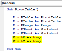
Step 6: Finally, to find the last used row & column, define two more variables as “Long.”
Code:
Dim LR As Long
Dim LC As Long
Step 7: We need to insert a new sheet to create a Pivot Table. Before that, if any pivot sheet is there, then we need to delete that.

Step 8: Now, set the object variable “PSheet” and “DSheet” to “Pivot Sheet” and “Data Sheet,” respectively.
![]()
Step 9: Find the last used row and last used column in the datasheet.

Step 10: Set the pivot range using the last row and last column.
![]()
It will set the data range perfectly. Furthermore, it will automatically select the data range, even if there is any addition or deletion of data in the datasheet.
Step 11: Before we create a PivotTable, we need to create a pivot cache. Set the pivot cache variable by using the below VBA codeVBA code refers to a set of instructions written by the user in the Visual Basic Applications programming language on a Visual Basic Editor (VBE) to perform a specific task.read more.
![]()
Step 12: Now, create a blank PivotTable.
![]()
Step 13: After inserting the PivotTable, we must insert the row field first. So, we will insert the row field as my ‘Country” column.
Note: Download the workbook to understand the data columns.

Step 14: We will insert one more item into the row field as the second position item. We will insert the “Product” as the second line item to the row field.

Step 15: After inserting the columns into the row field, we need to insert values into the column field. We will insert the “Segment” into the column field.

Step 16: We need to insert numbers into the data field. So insert “Sales” into the data field.

Step 17: We have completed the Pivot Table summary part. Now, we need to format the table. To format the pivot table, use the below code.

Note: To have more different table styles record them macro and get the table styles.
To show the row field values items in tabular form, add the below code at the bottom.

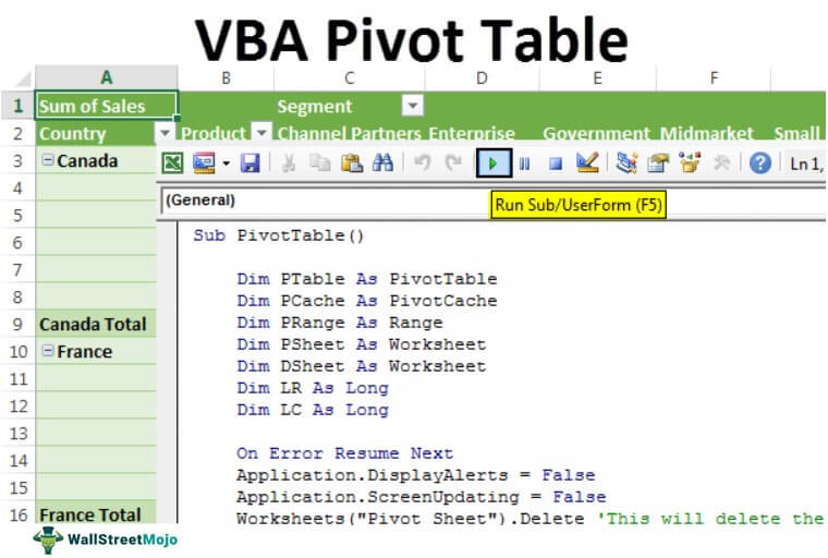
We have completed it now. If we run this code using the F5 key or manually, we should get the PivotTable like this.

Like this, we can automate creating a PivotTable using VBA coding.
For your reference, we have given the code below.
Sub PivotTable()

Dim PTable As PivotTable
Dim PCache As PivotCache
Dim PRange As Range
Dim PSheet As Worksheet
Dim DSheet As Worksheet
Dim LR As Long
Dim LC As Long

On Error Resume NextVBA On Error Resume Statement is an error-handling aspect used for ignoring the code line because of which the error occurred and continuing with the next line right after the code line with the error.read more
Application.DisplayAlerts = False
Application.ScreenUpdating = False
Worksheets("Pivot Sheet").Delete 'This will delete the exisiting pivot table worksheet
Worksheets.Add After:=ActiveSheet ' This will add new worksheet
ActiveSheet.Name = "Pivot Sheet" ' This will rename the worksheet as "Pivot Sheet"
On Error GoTo 0

Set PSheet = Worksheets("Pivot Sheet")
Set DSheet = Worksheets("Data Sheet")

'Find Last used row and column in data sheet
LR = DSheet.Cells(Rows.Count, 1).End(xlUp).Row
LC = DSheet.Cells(1, Columns.Count).End(xlToLeft).Column

'Set the pivot table data range
Set PRange = DSheet.Cells(1, 1).Resize(LR, LC)

'Set pivot cahe
Set PCache = ActiveWorkbook.PivotCaches.Create(xlDatabase, SourceData:=PRange)

'Create blank pivot table
Set PTable = PCache.CreatePivotTable(TableDestination:=PSheet.Cells(1, 1), TableName:="Sales_Report")

'Insert country to Row Filed
With PSheet.PivotTables("Sales_Report").PivotFields("Country")
.Orientation = xlRowField
.Position = 1
End With

'Insert Product to Row Filed & position 2
With PSheet.PivotTables("Sales_Report").PivotFields("Product")
.Orientation = xlRowField
.Position = 2
End With

'Insert Segment to Column Filed & position 1
With PSheet.PivotTables("Sales_Report").PivotFields("Segment")
.Orientation = xlColumnField
.Position = 1
End With

'Insert Sales column to the data field
With PSheet.PivotTables("Sales_Report").PivotFields("Sales")
.Orientation = xlDataField
.Position = 1
End With

'Format Pivot Table
PSheet.PivotTables("Sales_Report").ShowTableStyleRowStripes = True
PSheet.PivotTables("Sales_Report").TableStyle2 = "PivotStyleMedium14"

'Show in Tabular form
PSheet.PivotTables("Sales_Report").RowAxisLayout xlTabularRow

Application.DisplayAlerts = True
Application.ScreenUpdating = True

End Sub
Recommended Articles
This article is a guide to the VBA Pivot Table. Here, we learn how to create a PivotTable in Excel using VBA code, a practical example, and a downloadable template. Below you can find some useful Excel VBA articles: –
- Filter in Pivot Table
- Pivot Table Calculated Field
- Multiple Sheets Pivot Table
- Slicer using Pivot Table
- VBA Web Scraping
Before I hand over this guide to you and you start using VBA to create a pivot table let me confess something.
I have learned using VBA just SIX years back. And the first time when I wrote a macro code to create a pivot table, it was a failure.
Since then, I have learned more from my bad coding rather than from the codes which actually work.
Today, I will show you a simple way to automate your pivot tables using a macro code.
Normally when you insert a pivot table in a worksheet it happens through a simple process, but that entire process is so quick that you never notice what happened.
In VBA, that entire process is same, just executes using a code. In this guide, I’ll show you each step and explain how to write a code for it.
Just look at the below example, where you can run this macro code with a button, and it returns a new pivot table in a new worksheet in a flash.
Without any further ado, let’s get started to write our macro code to create a pivot table.
The Simple 8 Steps to Write a Macro Code in VBA to Create a Pivot Table in Excel
For your convenience, I have split the entire process into 8 simple steps. After following these steps you will able to automate your all the pivot tables.
Make sure to download this file from here to follow along.
1. Declare Variables
The first step is to declare the variables which we need to use in our code to define different things.
'Declare Variables
Dim PSheet As Worksheet
Dim DSheet As Worksheet
Dim PCache As PivotCache
Dim PTable As PivotTable
Dim PRange As Range
Dim LastRow As Long
Dim LastCol As Long
In the above code, we have declared:
- PSheet: To create a sheet for a new pivot table.
- DSheet: To use as a data sheet.
- PChache: To use as a name for pivot table cache.
- PTable: To use as a name for our pivot table.
- PRange: to define source data range.
- LastRow and LastCol: To get the last row and column of our data range.
2. Insert a New Worksheet
Before creating a pivot table, Excel inserts a blank sheet and then create a new pivot table there.

And, below code will do the same for you.
It will insert a new worksheet with the name “Pivot Table” before the active worksheet and if there is worksheet with the same name already, it will delete it first.
After inserting a new worksheet, this code will set the value of PSheet variable to pivot table worksheet and DSheet to source data worksheet.
'Declare Variables
On Error Resume Next
Application.DisplayAlerts = False
Worksheets("PivotTable").Delete
Sheets.Add Before:=ActiveSheet
ActiveSheet.Name = "PivotTable"
Application.DisplayAlerts = True
Set PSheet = Worksheets("PivotTable")
Set DSheet = Worksheets("Data")
Customization Tip: If the name of the worksheets which you want to refer in the code is different then make sure to change it from the code where I have highlighted.
3. Define Data Range
Now, next thing is to define data range from the source worksheet. Here you need to take care of one thing that you can’t specify a fixed source range.
You need a code which can identify the entire data from source sheet. And below is the code:
'Define Data Range
LastRow = DSheet.Cells(Rows.Count, 1).End(xlUp).Row
LastCol = DSheet.Cells(1, Columns.Count).End(xlToLeft).Column
Set PRange = DSheet.Cells(1, 1).Resize(LastRow, LastCol)
This code will start from the first cell of the data table and select up to the last row and then up to the last column.
And finally, define that selected range as a source. The best part is, you don’t need to change data source every time while creating the pivot table.
4. Create Pivot Cache
In Excel 2000 and above, before creating a pivot table you need to create a pivot cache to define the data source.
Normally when you create a pivot table, Excel automatically creates a pivot cache without asking you, but when you need to use VBA, you need to write a code for this.
'Define Pivot Cache
Set PCache = ActiveWorkbook.PivotCaches.Create _
(SourceType:=xlDatabase, SourceData:=PRange). _
CreatePivotTable(TableDestination:=PSheet.Cells(2, 2), _
TableName:="SalesPivotTable")
This code works in two ways, first define a pivot cache by using data source and second define the cell address in the newly inserted worksheet to insert the pivot table.
You can change the position the pivot table by editing this code.
5. Insert a Blank Pivot Table
After pivot cache, next step is to insert a blank pivot table. Just remember when you create a pivot table what happens, you always get a blank pivot first and then you define all the values, columns, and row.

This code will do the same:
'Insert Blank Pivot Table
Set PTable = PCache.CreatePivotTable _
(TableDestination:=PSheet.Cells(1, 1), TableName:="SalesPivotTable")
This code creates a blank pivot table and names it “SalesPivotTable”. You can change this name from the code itself.
6. Insert Row and Column Fields
After creating a blank pivot table, next thing is to insert row and column fields, just like you do normally.
For each row and column field, you need to write a code. Here we want to add years and month in row field and zones in the column field.

Here is the code:
'Insert Row Fields
With ActiveSheet.PivotTables("SalesPivotTable").PivotFields("Year")
.Orientation = xlRowField
.Position = 1
End With

With ActiveSheet.PivotTables("SalesPivotTable").PivotFields("Month")
.Orientation = xlRowField
.Position = 2
End With

'Insert Column Fields
With ActiveSheet.PivotTables("SalesPivotTable").PivotFields("Zone")
.Orientation = xlColumnField
.Position = 1
End With
In this code, you have mentioned year and month as two fields. Now, if you look at the code, you’ll find that a position number is also there. This position number defines the sequence of fields.
Whenever you need to add more than one field (Row or Column), specify their position. And you can change fields by editing their name from the code.
7. Insert Data Field
The main thing is to define the value field in your pivot table.
The code for defining values differs from defining rows and columns because we must define the formatting of numbers, positions, and functions here.
'Insert Data Field
With ActiveSheet.PivotTables("SalesPivotTable").PivotFields("Amount")
.Orientation = xlDataField
.Function = xlSum
.NumberFormat = "#,##0"
.Name = "Revenue "
End With
You can add the amount as the value field with the above code. And this code will format values as a number with a (,) separator.
We use xlsum to sum values, but you can also use xlcount and other functions.
8. Format Pivot Table
Ultimately, you need to use a code to format your pivot table. Typically there is a default formatting in a pivot table, but you can change that formatting.
With VBA, you can define formatting style within the code.

Code is:
'Format Pivot
TableActiveSheet.PivotTables("SalesPivotTable").ShowTableStyleRowStripes = True
ActiveSheet.PivotTables("SalesPivotTable").TableStyle2 = "PivotStyleMedium9"
The above code will apply row strips and the “Pivot Style Medium 9” style, but you can also use another style from this link.
Finally, your code is ready to use.
[FULL CODE] Use VBA to Create a Pivot Table in Excel – Macro to Copy-Paste
Sub InsertPivotTable()
'Macro By ExcelChamps.com

'Declare Variables
Dim PSheet As Worksheet
Dim DSheet As Worksheet
Dim PCache As PivotCache
Dim PTable As PivotTable
Dim PRange As Range
Dim LastRow As Long
Dim LastCol As Long

'Insert a New Blank Worksheet
On Error Resume Next
Application.DisplayAlerts = False
Worksheets("PivotTable").Delete
Sheets.Add Before:=ActiveSheet
ActiveSheet.Name = "PivotTable"
Application.DisplayAlerts = True
Set PSheet = Worksheets("PivotTable")
Set DSheet = Worksheets("Data")

'Define Data Range
LastRow = DSheet.Cells(Rows.Count, 1).End(xlUp).Row
LastCol = DSheet.Cells(1, Columns.Count).End(xlToLeft).Column
Set PRange = DSheet.Cells(1, 1).Resize(LastRow, LastCol)

'Define Pivot Cache
Set PCache = ActiveWorkbook.PivotCaches.Create _
(SourceType:=xlDatabase, SourceData:=PRange). _
CreatePivotTable(TableDestination:=PSheet.Cells(2, 2), _
TableName:="SalesPivotTable")

'Insert Blank Pivot Table
Set PTable = PCache.CreatePivotTable _
(TableDestination:=PSheet.Cells(1, 1), TableName:="SalesPivotTable")

'Insert Row Fields
With ActiveSheet.PivotTables("SalesPivotTable").PivotFields("Year")
.Orientation = xlRowField
.Position = 1
End With
With ActiveSheet.PivotTables("SalesPivotTable").PivotFields("Month")
.Orientation = xlRowField
.Position = 2
End With

'Insert Column Fields
With ActiveSheet.PivotTables("SalesPivotTable").PivotFields("Zone")
.Orientation = xlColumnField
.Position = 1
End With

'Insert Data Field
With ActiveSheet.PivotTables("SalesPivotTable").PivotFields ("Amount")
.Orientation = xlDataField
.Function = xlSum
.NumberFormat = "#,##0"
.Name = "Revenue "
End With

'Format Pivot Table
ActiveSheet.PivotTables("SalesPivotTable").ShowTableStyleRowStripes = True
ActiveSheet.PivotTables("SalesPivotTable").TableStyle2 = "PivotStyleMedium9"

End Sub
Download Sample File
- Ready
Pivot Table on the Existing Worksheet
The code we have used above creates a pivot table on a new worksheet, but sometimes you need to insert a pivot table in a worksheet already in the workbook.
In the above code (Pivot Table in New Worksheet), in the part where you have written the code to insert a new worksheet and then name it. Please make some tweaks to the code.
Don’t worry; I’ll show you.
You first need to specify the worksheet (already in the workbook) where you want to insert your pivot table.
And for this, you need to use the below code:
Instead of inserting a new worksheet, you must specify the worksheet name to the PSheet variable.
Set PSheet = Worksheets("PivotTable")
Set DSheet = Worksheets(“Data”)
There is a bit more to do. The first code you used deletes the worksheet with the same name (if it exists) before inserting the pivot.
When you insert a pivot table in the existing worksheet, there’s a chance that you already have a pivot there with the same name.
What I’m saying is you need to delete that pivot first.
For this, you need to add the code which should delete the pivot with the same name from the worksheet (if it’s there) before inserting a new one.
Here’s the code which you need to add:
Set PSheet = Worksheets("PivotTable")
Set DSheet = Worksheets(“Data”)
Worksheets("PivotTable").Activate
On Error Resume Next
ActiveSheet.PivotTables("SalesPivotTable").TableRange2.Clear
Let me tell you what this code does.
First, it simply sets PSheet as the worksheet where you want to insert the pivot table already in your workbook and sets data worksheets as DSheet.
After that, it activates the worksheet and deletes the pivot table “Sales Pivot Table” from it.
Important: If the worksheets’ names in your workbook differ, you can change them from the code. I have highlighted the code where you need to do it.
In the End,
By using this code, we can automate your pivot tables. And the best part is this is a one-time setup; after that, we just need a click to create a pivot table and you can save a ton of time. Now tell me one thing.
Have you ever used a VBA code to create a pivot table?
Please share your views with me in the comment box; I’d love to share them with you and share this tip with your friends.
VBA is one of the Advanced Excel Skills, and if you are getting started with VBA, make sure to check out there and Useful Macro Examples and VBA Codes.
- Add or Remove Grand Total in a Pivot Table in Excel
- Add Running Total in a Pivot Table in Excel
- Automatically Update a Pivot Table in Excel
- Add Calculated Field and Item
- Delete a Pivot Table in Excel
- Filter a Pivot Table in Excel
- Add Ranks in Pivot Table in Excel
- Apply Conditional Formatting to a Pivot Table in Excel
- Create Pivot Table using Multiple Files in Excel
- Change Data Source for Pivot Table in Excel
- Count Unique Values in a Pivot Table in Excel
- Pivot Chart in Excel
- Create a Pivot Table from Multiple Worksheets
- Sort a Pivot Table in Excel
- Refresh All Pivot Tables at Once in Excel
- Refresh a Pivot Table
- Pivot Table Timeline in Excel
- Pivot Table Keyboard Shortcuts
- Pivot Table Formatting
- Move a Pivot Table
- Link a Slicer with Multiple Pivot Tables in Excel
- Group Dates in a Pivot Table in Excel
Pivot Tables are a key tool for many Excel users to analyze data. They are flexible and easy to use. Combine the power of Pivot Tables with the automation of VBA, and we can analyze data even faster. This post includes the essential code to control Pivot Tables with VBA.
Download the example file
I recommend you download the example file for this post. Then you’ll be able to work along with examples and see the solution in action, plus the file will be useful for future reference.
![]()
Download the file: 0047 Excel VBA for Pivot Tables.zip
Refreshing Pivot Tables
Of all the tasks we undertake on Pivot Tables, refreshing the data is the most common. So, let’s start there.
Refresh a Pivot Table
The following code refreshes a single Pivot Table called PivotTable1. Change the value of the pvtName variable to be the name of your Pivot Table.
Sub RefreshAPivotTable()

'Create a variable to hold name of Pivot Table
Dim pvtName As String

'Assign Pivot Table name to variable
pvtName = "PivotTable1"

'Refresh the Pivot Table
ActiveSheet.PivotTables(pvtName).PivotCache.Refresh
End Sub
Refresh all the Pivot Tables in the active workbook
The next code snippet refreshes all Pivot Tables in the active workbook.
Sub RefreshAllPivotTables()

'Refresh all Pivot Tables
ActiveWorkbook.RefreshAll

End Sub
Refresh all the Pivot Tables on a worksheet
We can refresh all the Pivot Tables in a workbook with a single line of code. However, to refresh all the Pivot Tables on a worksheet, we need to loop through and refresh each one.
Sub RefreshAllPivotTablesWorkbook()

'Create a variable to hold worksheets
Dim ws As Worksheet

'Create a variable to hold Pivot Tables
Dim pvt As PivotTable

'Loop through each worksheet
For Each ws In ActiveWorkbook.Worksheets

    'Loop through each Pivot Table
    For Each pvt In ws.PivotTables

        'refresh the Pivot Table
        pvt.RefreshTable

    Next pvt

Next ws

End Sub
Create a Pivot Table
The following VBA code creates a Pivot Table. It requires 4 inputs:
- The sheet containing the source data
- The range containing the source data
- The sheet on which to place the Pivot Table
- The cell reference where to place the Pivot Table
Sub CreatePivotTable()

'Create all the variables
Dim pvtCache As PivotCache
Dim pvt As PivotTable
Dim pvtLocationWs As String
Dim pvtLocationRng As String
Dim pvtSourceWs As String
Dim pvtSourceRng As String
Dim pvtSourceFull As String
Dim pvtLocationFull As String

'Set the sheet and ranges for the variables
pvtSourceWs = "Sheet1"
pvtSourceRng = "A1:D50"
pvtLocationWs = "Sheet2"
pvtLocationRng = "A1"

'Create the string for the source
pvtSourceFull = pvtSourceWs & "!" & _
    Range(pvtSourceRng).Address(ReferenceStyle:=xlR1C1)

'Create the string for the location
pvtLocationFull = pvtLocationWs & "!" & _
    Range(pvtLocationRng).Address(ReferenceStyle:=xlR1C1)

'Create the Pivot Cache
Set pvtCache = ActiveWorkbook.PivotCaches.Create(SourceType:=xlDatabase, _
    SourceData:=pvtSourceFull)

'Create the Pivot Table
Set pvt = pvtCache.CreatePivotTable(TableDestination:=pvtLocationFull, _
    TableName:="PivotTable1")

End Sub
The example above uses standard Excel ranges. To use an Excel Table as the source, we can use the Table’s name without referencing the sheet.
Deleting Pivot Tables
This section contains two options for deleting Pivot Tables.
Delete a single Pivot Table
The following macro deletes a single Pivot Table. Change the name of the pvtName variable to the name of the Pivot Table you wish to delete.
Sub DeletePivotTable()

'Create a variable to hold name of Pivot Table
Dim pvtName As String

'Assign Pivot Table name to variable
pvtName = "PivotTable1"

'Delete the Pivot Table named PivotTable1
ActiveSheet.PivotTables(pvtName).TableRange2.Clear

End Sub
Delete all Pivot Tables in the workbook
While we can refresh all Pivot Tables in one go, to delete Pivot Tables, we must loop through and delete each.
Sub DeleteAllPivotTable()

'Create a variable to hold worksheets
Dim ws As Worksheet

'Create a variable to hold Pivot Tables
Dim pvt As PivotTable

'Loop through each sheet in the activeworkbook
For Each ws In ActiveWorkbook.Worksheets

    'Loop through each Pivot Table in the worksheet
    For Each pvt In ws.PivotTables

        'Turn off auto fit
        pvt.TableRange2.Clear

    Next pvt

Next ws

End Sub
Change Pivot Table Source
This macro changes the source data for a Pivot Table.
Sub ChangePivotTableSource()

'Create all the variables
Dim pvtCache As PivotCache
Dim pvt As PivotTable
Dim pvtName As String
Dim pvtSourceWs As String
Dim pvtSourceRng As String
Dim pvtSourceFull As String

'Set the sheet and ranges for the variables
pvtName = "PivotTable1"
pvtSourceWs = "Sheet1"
pvtSourceRng = "H1:K4"

Set pvt = ActiveSheet.PivotTables(pvtName)

'Create the string for the source
pvtSourceFull = pvtSourceWs & "!" & _
    Range(pvtSourceRng).Address(ReferenceStyle:=xlR1C1)

'Create a new Pivot Cache
Set pvtCache = ActiveWorkbook.PivotCaches.Create(SourceType:=xlDatabase, _
    SourceData:=pvtSourceFull)

'Change Pivot Cache the Pivot Table is pointed to
pvt.ChangePivotCache pvtCache

End Sub
The example above uses standard Excel ranges. To use an Excel Table as the source we can use the Table’s name without referencing the sheet.
Turn off autofit column widths on all Pivot Tables
The following macro changes the settings to retain column widths when a Pivot Table is refreshed.
Sub TurnOffAutoFitColumnsPivotTables()

'Create a variable to hold worksheets
Dim ws As Worksheet

'Create a variable to hold Pivot Tables
Dim pvt As PivotTable

'Loop through each sheet in the activeworkbook
For Each ws In ActiveWorkbook.Worksheets

    'Loop through each Pivot Table in the worksheet
    For Each pt In ws.PivotTables

        'Turn off auto fit
        pvt.HasAutoFormat = False
        'Turn auto fit back on
        'pvt.HasAutoFormat = True

    Next pvt

Next ws

End Sub
Adding and removing columns, rows and values to a Pivot Table
After creating a Pivot Table, we then need to add/remove fields and apply filters to get the view that we want.
Add fields to a Pivot Table
Sub AddFieldToPivotTableRows()

Dim pvt As PivotTable
Dim pvtFieldName As String

Set pvt = ActiveSheet.PivotTables("PivotTable1")
pvtFieldName = "Customer Name"

pvt.PivotFields(pvtFieldName).Orientation = xlRowField

End Sub
Add field to Pivot Table columns
Sub AddFieldToPivotTableColumns()

Dim pvt As PivotTable
Dim pvtFieldName As String

Set pvt = ActiveSheet.PivotTables("PivotTable1")
pvtFieldName = "Customer Name"

pvt.PivotFields(pvtFieldName).Orientation = xlColumnField

End Sub
Add field to Pivot Table filters
Sub AddFieldToPivotTableFilters()

Dim pvt As PivotTable
Dim pvtFieldName As String

Set pvt = ActiveSheet.PivotTables("PivotTable1")
pvtFieldName = "Customer Name"

pvt.PivotFields(pvtFieldName).Orientation = xlPageField

End Sub
Position field in Pivot Table filters
Sub PostionFieldInPivotTableFilters()

Dim pvt As PivotTable
Dim pvtFieldName As String

Set pvt = ActiveSheet.PivotTables("PivotTable1")
pvtFieldName = "Customer Name"

pvt.PivotFields(pvtFieldName).Position = 1

End Sub
Remove field from Pivot Table values
Sub RemoveFieldFromPivotTableValues()

Dim pvt As PivotTable
Dim pvtFieldName As String

Set pvt = ActiveSheet.PivotTables("PivotTable1")
pvtFieldName = "Customer Name"

pvt.PivotFields(pvtFieldName).Orientation = xlHidden

End Sub
Position field in a Pivot Table
Sub PostionFieldInPivotTable()

Dim pvt As PivotTable
Dim pvtFieldName As String

Set pvt = ActiveSheet.PivotTables("PivotTable1")
pvtFieldName = "Customer Name"

pvt.PivotFields(pvtFieldName).Position = 1

End Sub
Add field to Pivot Table values section
Sub AddFieldToPivotTableValues()

Dim pvt As PivotTable
Dim pvtFieldName As String
Dim pvtFieldDescription As String

Set pvt = ActiveSheet.PivotTables("PivotTable1")
pvtFieldName = "Revenue"
pvtFieldDescription = "Sum of Revenue"

pvt.AddDataField pvt.PivotFields(pvtFieldName), pvtFieldDescription, xlSum

End Sub
Remove field from Pivot Table values section
Sub RemoveValueFieldFromPivotTableValues()

Dim pvt As PivotTable
Dim pvtFieldDescription As String

Set pvt = ActiveSheet.PivotTables("PivotTable1")
pvtFieldDescription = "Sum of Revenue"

pvt.PivotFields(pvtFieldDescription).Orientation = xlHidden

End Sub
Clear Pivot Tables filters
Sub ClearFiltersToPivotTable()

Dim pvt As PivotTable
Dim pvtField As PivotField
Dim pvtFieldName As String
Dim pvtName As String

pvtName = "PivotTable1"
Set pvt = ActiveSheet.PivotTables(pvtName)

pvtFieldName = "Customer Name"
Set pvtField = pvt.PivotFields(pvtFieldName)

pvtField.ClearAllFilters

End Sub
Apply filter to Pivot Table
Sub ApplyFilterToPivotTable()

Dim pvt As PivotTable
Dim pvtField As PivotField
Dim pvtFieldName As String
Dim pvtName As String
Dim pvtFilter As String

pvtName = "PivotTable1"
Set pvt = ActiveSheet.PivotTables(pvtName)

pvtFieldName = "Customer Name"
Set pvtField = pvt.PivotFields(pvtFieldName)

pvtFilter = "A"

pvtField.ClearAllFilters
pvtField.CurrentPage = pvtFilter

End Sub
Apply multiple filters to a Pivot Table
Sub ApplyMultipleFiltersToPivotTable()

Dim pvt As PivotTable
Dim pvtField As PivotField
Dim pvtItems As PivotItems
Dim pvtFieldName As String
Dim pvtName As String
Dim pvtFilters As Variant
Dim i As Integer
Dim j As Integer

pvtName = "PivotTable1"
Set pvt = ActiveSheet.PivotTables(pvtName)

pvtFieldName = "Customer Name"
Set pvtField = pvt.PivotFields(pvtFieldName)

pvtFilters = "A, B"

pvtFilters = Split(pvtFilters, ", ")

pvtField.ClearAllFilters

pvtField.EnableMultiplePageItems = True

For i = 1 To pvtField.PivotItems.Count

    For j = LBound(pvtFilters) To UBound(pvtFilters)

        If pvtField.PivotItems(i) = pvtFilters(j) Then

            pvtField.PivotItems(i).Visible = True
            Exit For

        Else

            pvtField.PivotItems(i).Visible = False

        End If

    Next j

Next i

End Sub
Add a calculated field
Sub AddCalculatedField()

Dim pvtName As String
Dim pvt As PivotTable
Dim pvtCalcName As String
Dim pvtCalc As String

pvtName = "PivotTable1"
Set pvt = ActiveSheet.PivotTables(pvtName)

pvtCalcName = "myCalculation1"
pvtCalc = "=Field1+Field2"

pvt.CalculatedFields.Add pvtCalcName, pvtCalc, True

End Sub
Clear all fields from a Pivot Table
Sub ClearAllFieldsFromPivotTable()

Dim pvtName As String
Dim pvt As PivotTable

pvtName = "PivotTable1"
Set pvt = ActiveSheet.PivotTables(pvtName)

pvt.ClearTable

End Sub

About the author
Hey, I’m Mark, and I run Excel Off The Grid.
My parents tell me that at the age of 7 I declared I was going to become a qualified accountant. I was either psychic or had no imagination, as that is exactly what happened. However, it wasn’t until I was 35 that my journey really began.
In 2015, I started a new job, for which I was regularly working after 10pm. As a result, I rarely saw my children during the week. So, I started searching for the secrets to automating Excel. I discovered that by building a small number of simple tools, I could combine them together in different ways to automate nearly all my regular tasks. This meant I could work less hours (and I got pay raises!). Today, I teach these techniques to other professionals in our training program so they too can spend less time at work (and more time with their children and doing the things they love).
Do you need help adapting this post to your needs?
I’m guessing the examples in this post don’t exactly match your situation. We all use Excel differently, so it’s impossible to write a post that will meet everybody’s needs. By taking the time to understand the techniques and principles in this post (and elsewhere on this site), you should be able to adapt it to your needs.
But, if you’re still struggling you should:
- Read other blogs, or watch YouTube videos on the same topic. You will benefit much more by discovering your own solutions.
- Ask the ‘Excel Ninja’ in your office. It’s amazing what things other people know.
- Ask a question in a forum like Mr Excel, or the Microsoft Answers Community. Remember, the people on these forums are generally giving their time for free. So take care to craft your question, make sure it’s clear and concise. List all the things you’ve tried, and provide screenshots, code segments and example workbooks.
- Use Excel Rescue, who are my consultancy partner. They help by providing solutions to smaller Excel problems.
What next?
Don’t go yet, there is plenty more to learn on Excel Off The Grid. Check out the latest posts: