

Форум программистов Vingrad
Новости ·
Фриланс ·
FAQ
Правила ·
Помощь ·
Рейтинг ·
Избранное ·
Поиск ·
Участники
Форум -> Компьютерные системы -> MS Office, Open Office и др. -> Программирование, связанное с MS Office
(еще)
| Модераторы: mihanik |
Поиск: |
  
|
|
Опции темы |

| Jonnik |
|
||
|
Шустрый Профиль Репутация: нет
|
Как програмно через VBA изменить направление текста в Excel с горизонтального на вертикальный? |
||
|
|||


| Genyaa |
|
||
|
Усердный Профиль
Репутация: 2
|
А как на счет того, чтобы записать макрорекордером это действие и посмотреть полученный код? ——————— Всякое решение плодит новые проблемы. |
||
|
|||

| Jonnik |
|
||
|
Шустрый Профиль Репутация: нет
|
Типа такого
|
||
|
|||


|
|
| Правила форума «Программирование, связанное с MS Office» | |
|
|
Запрещается! 1. Публиковать ссылки на вскрытые компоненты 2. Обсуждать взлом компонентов и делиться вскрытыми
Если Вам понравилась атмосфера форума, заходите к нам чаще! |

| 0 Пользователей читают эту тему (0 Гостей и 0 Скрытых Пользователей) |
| 0 Пользователей: |
| « Предыдущая тема | Программирование, связанное с MS Office | Следующая тема » |
Подписаться на тему |
Подписка на этот форум |
Скачать/Распечатать тему
[ Время генерации скрипта: 0.1123 ] [ Использовано запросов: 21 ] [ GZIP включён ]
Реклама на сайте
Информационное спонсорство
- Remove From My Forums
-
Question
-
Hi,
I’m using Office Interop to create an Excel workbook in code using C#.
One of the requirements is that some text which serves as headers are rotated 90 degrees.
In excel it’s Format Cells -> Alignment -> Orientation -> Degrees.
Does anyone know how I can achieve this using C# with Interop?
T.i.a.,
ratjetoes.
Answers
-
Within the Excel Object Model, text orientation is just another read/write property of the Range object. Using VBA:
Sub SlantText()
Dim r As Range
Set r = Range(«B9»)
With r
.Value = «Hello World»
.Orientation = 90
End With
End SubSo if you can set the value of a cell using C++, orientation should be similar.
-
Marked as answer by
Thursday, June 24, 2010 11:57 AM
-
Marked as answer by
In this article I will explain how you can change the orientation of the content in cells. I have also provided several sample codes.
Jump To:
- Example 1, Basics
- Example 2, Set Orientation
- Example 3, Get Orientation
You can download the file and code related to this article here.
–
Example 1, Basics:
The following code applies a 28 deg orientation to the contents of cell A1:
Range("A1").Orientation = 28
Before:

Result:

–
Example 2, Set Orientation:
In this example in row 1 the user selects the orientation to apply to the content of the cells in row 2:
Before:

After:

The program uses a worksheet_change event handler. The event handler executes when the user makes changes to the worksheet:
'executes when the user makes changes to the worksheet

Private  Sub  worksheet_Change(ByVal  target As  Range)

Dim  i As  Integer

For  i = 1 To  6

    'loops through all the columns

    Range(Cells(2, i), Cells(2, i)).Orientation = Cells(1, i)

Next  i

End  Sub
–
Example 3, Get Orientation:
In this example the user selects a lower and upper bound for the orientation. The program checks the orientation of the content in row 2. If the orientation falls between the upper and lower bounds selected by the user the cell in the next row is colored green:

By reducing the lower bound more cells will be colored green:

By increasing the upper bound more cells will be colored green:

The program uses a worksheet_change event handler. The event handler executes when the user makes changes to the worksheet:
'executes when the user makes changes to the worksheet

Private  Sub  worksheet_Change(ByVal  target As  Range)

Dim  i As  Integer

For  i = 1 To  6

    'checks if the orientation of the content in the cell under

    'consideration is between the upper and lower bounds selected by

    'the user

    If  (Range(Cells(2, i), Cells(2, i)).Orientation <= Cells(1, 4)) _

    And (Range(Cells(2, i), Cells(2, i)).Orientation >= Cells(1, 2)) Then

        Range(Cells(3, i), Cells(3, i)).Interior.Color = 3394611

    Else

        Range(Cells(3, i), Cells(3, i)).Interior.Pattern = xlNone

    End If

Next  i

End  Sub
The line below colors the cell green. The number 3394611 is a color code. This was obtained using the macro recorder. For more information about about the macro recorder please see Excel VBA Formatting Cells and Ranges Using the Macro Recorder:
Range(Cells(3, i), Cells(3, i)).Interior.Color = 3394611
The line below removes any fill color previously assigned to the cell:
Range(Cells(3, i), Cells(3, i)).Interior.Pattern = xlNone
You can download the file and code related to this article here.
See also:
- VBA Excel, Alignment
If you need assistance with your code, or you are looking for a VBA programmer to hire feel free to contact me. Also please visit my website www.software-solutions-online.com
|
Группа: Друзья Ранг: Экселист Сообщений: 8132
Замечаний: |

Цитата stepan190, 04.05.2020 в 13:17, в сообщении № 1 ()
всех ячейках
лень что-то,
для выделенных
[vba]
Код
Sub u_751()
Application.ScreenUpdating = False
For Each c In Selection
If c.Orientation <> -4128 Then
c.Interior.Color = 255
c.Orientation = 0
End If
Next
Application.ScreenUpdating = True
End Sub
[/vba]
ЮMoney 41001841029809
Reversing a string may not have many real-world applications, especially when working with spreadsheets. That is why you will not find any built-in function for this in Excel.
But there might be cases where you need to reverse a string, for whatever reason. Maybe you need to generate a special code, maybe you need to see if a string is a palindrome, or maybe you just want to do it for fun.
Even though there aren’t any built-in Excel functions for string reversal, there are a number of different ways to do this. You can use either a formula or a script written in VBA.
In this tutorial, we will see two ways to reverse a text string using a formula. If you like to use macros, then we also have a VBA script to help you reverse multiple strings quickly.
Reversing Text String using Text Formulas
Let us first understand the main process involved in reversing a string.
Let’s say you have a single cell with text that you want to reverse.
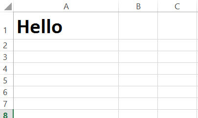
To reverse the string “Hello” in cell A1, follow these steps:
- In cell B1, type the following formula: =MID($A$1,LEN($A$1)-ROW(B1)+1,1). This should return the last character in the given string, which is “o”.
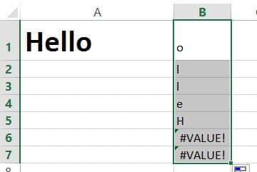
- Drag the fill handle down (situated at the bottom right of cell B1) until you start seeing “#VALUE!”.

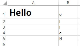
- You should now see each character of the string in “Hello” in each cell of column B, but reversed. Clear any cells containing “#VALUE!”. Here’s what you should finally see in our example:

- After the last cell of column B, i.e. in cell B6, type the formula: =TRANSPOSE(
- Drag and select the cells B1 to B5.
- Close the parentheses for the TRANSPOSE formula.
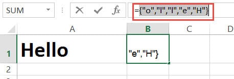
- Now select the whole formula in the formula bar and press F9 on your keyboard. This should display the values of each cell from B1 to B5, separated by commas and the whole thing should be surrounded by curly brackets: {“o”,”l”,”l”,”e”,”H”}.
- Remove the opening and closing curly brackets.
- Type “CONCATENATE”, followed by opening parentheses after the equal to sign.
- Close the parentheses after “H”.
- Press the return key.
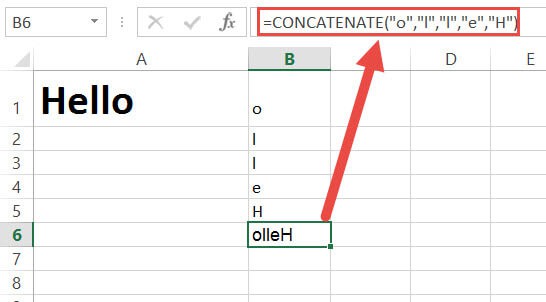
You should now see the reverse of the string “Hello” in cell B6.
What happened here?
Now let us look at what the formula did.
=MID($A$1,LEN($A$1)-ROW(B1)+1,1)
The function LEN($A$1) returns the length of the string in cell A1. We don’t want this cell reference to change when copied to the cells below B1, so we locked the cell reference by adding ‘$’ signs to it. The length of the string “Hello” is 5, so this function will return the value, ‘5’.
The function ROW(B1) simply returns the row number of cell B1. We might as well have typed ‘1’ instead of ‘ROW(B1)’, but wanted this value to change each time it was copied to a new cell. So when it’s copied to cell B2, it changes to value ‘2’. When copied to cell B3, it changed to value ‘3’ and so on.
Now, LEN($A$1)-ROW(B1)+1 gives us the value ‘5’, which is the index of the last character in “Hello”.
The function MID() returns the characters at a given index. It takes three parameters – A string or reference to a string, an index, and the number of characters to return starting at that index.
Here, the formula =MID($A$1,LEN($A$1)-ROW(B1)+1,1) takes the reference to cell A1 as the first parameter, the index, 5 as the second parameter and the number 1, as the third parameter. So the formula returns the character at index 5 of cell A1. This means we get the value “o” – the last character of the string.
Here’s what’s happening when you break down the formula:
- =MID($A$1,LEN($A$1)-ROW(B1)+1,1)
- =MID($A$1, 5 – 1 + 1, 1)
- =MID($A$1, 5, 1)
- =”o”
What happens when the formula is copied to cell B2?
In cell B2, the formula now changes to:
=MID($A$1,LEN($A$1)-ROW(B2)+1,1)
Here’s what’s happening when you break down the formula:
- =MID($A$1,LEN($A$1)-ROW(B2)+1,1)
- =MID($A$1, 5 – 2 + 1, 1)
- =MID($A$1, 4, 1)
- =”l”
What happens when the formula is copied to cell B5?
In cell B5, the formula now changes to:
=MID($A$1,LEN($A$1)-ROW(B5)+1,1)
Here’s what’s happening when you break down the formula:
- =MID($A$1,LEN($A$1)-ROW(B5)+1,1)
- =MID($A$1, 5 – 5 + 1, 1)
- =MID($A$1, 1, 1)
- =”H”
So the function returns the first character of the string in A1.
Although the above method works fine, it is not very practical as you would need to involve a whole lot of cells in your sheet. We demonstrated the above method just to break down the technique and make it easy for you to understand what’s happening.
Here’s a shortened down and more practical version of the above technique:
- In cell B1, type the formula:
=TRANSPOSE(MID(A1,LEN(A1)-ROW(INDIRECT("1:"&LEN(A1)))+1,1)) in cell B1. - Select the entire formula in the formula bar and press F9 on your keyboard.
- This should display each character of your string, reversed and separated by commas. The whole thing should be also surrounded by curly brackets, which means this is an array: {“o”,”l”,”l”,”e”,”H”}.

- Remove the opening and closing curly brackets.
- Type “CONCATENATE”, followed by opening parentheses after the equal to sign.
- Close the parentheses after “H”.
- Press the return key.

You should now see the reverse of the string “Hello” in cell B1. This calculation got done directly and in one cell. So it is a much more efficient way of using the formula to reverse a string.
There are a few things to note about this technique though:
- The reversed string will not change when you change the value in cell A1. You will need to repeat this process every time there’s a change.
- This method is alright if you have a few strings that you want to reverse, but if you have a whole list of strings to reverse, it might prove to be a little painstaking. This is because you need to always repeat steps 2 to 7 for every string.
Due to the above 2 disadvantages, we recommend using a VBA script to reverse text string in Excel.
Reversing Characters of a Text String in Excel using VBA Macro
Using VBA might sound a little intimidating if you’ve never used it before, but it can be an easier method to reverse strings in your worksheet.
Here’s the VBA code that we will be used to reverse a string in a single cell. Feel free to select and copy it.
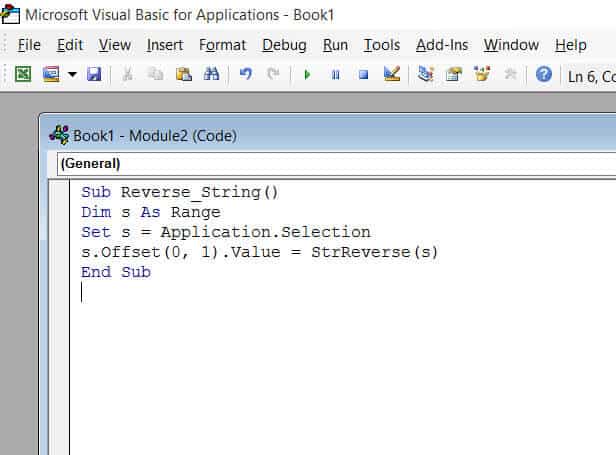
Sub Reverse_String()
Dim s As Range
Set s = Application.Selection
s.Offset(0, 1).Value = StrReverse(s)
End Sub
Follow these steps:
- From the Developer Menu Ribbon, select Visual Basic.
- Once your VBA window opens, Click Insert->Module. Now you can start coding. Type or copy-paste the above lines of code into the module window. Your code is now ready to run.

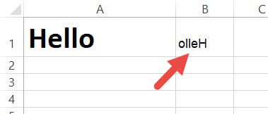
- Select a single cell containing the text you want to reverse. Make sure the cell horizontally next to it is blank because this is where the macro will display the reversed string.
- Navigate to Developer->Macros->Reverse_String->Run.

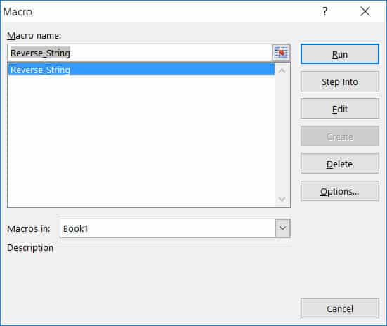
You will now see the reversed string next to your selected cell.
Note: If you can’t see the Developer ribbon, from the File menu, go to Options. Select Customize Ribbon and check the Developer option from the Main Tabs.
Finally, Click OK.
Reversing a List of Strings in Excel using VBScript
Using VBScript to reverse a long list of strings is easy too! Say you want to reverse the following set of names:
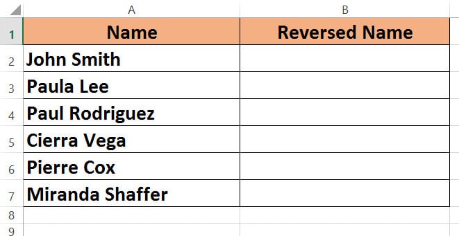
Here’s the VBA code that we will be using to reverse all strings in a column. Select and copy it.
Sub reverse_string_range()
Dim s As Range
Dim cell As Range
Set s = Application.Selection
i = 0
For Each cell In s
cell.Offset(0, 1).Value = StrReverse(cell)
i = i + 1
Next cell
End Sub
Follow these steps:
- From the Developer Menu Ribbon, select Visual Basic.
- Once your VBA window opens, Click Insert->Module. Now you can start coding. Type or copy-paste the above lines of code into the module window. Your code is now ready to run.
- Select the range of cells containing the text you want to reverse. Make sure the column next to it is blank because this is where the macro will display the reversed strings.
- Navigate to Developer->Macros->reverse_string_range->Run.
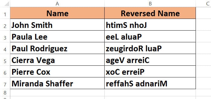
You will now see the reversed strings next to your selected range of cells.
Do remember to keep a backup of your sheet, because the results of VBA code are usually irreversible.
To wrap it up, we saw two ways to reverse strings in Excel. One method uses a formula and the other method uses VBA code.
The first method is alright if you don’t really feel comfortable working with VBA code. But it is beneficial only if you have one or a few cells that you want to reverse.
If there are more cells that need to be reversed, it can prove to be time-consuming.
Instead, you can use the second method (using VBA code), because it saves time and with just a few clicks, you can get a whole list of strings reversed in one go.
Although there are no straight ways to reverse a text string in Excel, I hope the methods shown here will help you get it done easily.
I hope you found this tutorial useful.
Other Excel tutorials you may find useful:
- How to Merge First and Last Name in Excel
- How to Split One Column into Multiple Columns in Excel
- How to Remove Commas in Excel (from Numbers or Text String)
- How to Generate Random Numbers in Excel (Without Duplicates)
- How to Add Text to the Beginning or End of all Cells in Excel
- How to Extract Number from Text in Excel (Beginning, End, or Middle)
- How to Change Uppercase to Lowercase in Excel
- How to Find the Last Space in Text String in Excel?
- Switch First and Last Name with Comma in Excel (Flip Names)
Хитрости »
4 Май 2011 57877 просмотров
Как перевернуть слово?
Не самая распространенная, но тем не менее встречающаяса задача: перевернуть слово. Т.е. расположить буквы слова в обратном порядке. Из «привет» сделать «тевирп». Если честно, то сейчас затрудняюсь озвучить конкретную ситуацию, в которой это может пригодиться. Сам использовал когда-то в случае, когда надо было перевернуть числовые значения с еще некоторыми манипуляциями. Но ситуации бывают разные, как и решения задачи, которых несколько.
Сначала я хотел бы описать способы переворачивания слова средствами VBA, т.к. именно они кажутся мне наиболее рациональными и наиболее удобными для большинства, несмотря на необходимость использовать VBA.
Способ 1:
Через встроенную функцию VBA StrReverse(). Быстрый и короткий. Самый удобный. Но работает только начиная от Excel 2000 и выше.
Sub Reverse_Word()
    On Error Resume Next
    ActiveCell.Value = StrReverse(ActiveCell.Value)
End Sub
Чтобы применить этот код необходимо слегка погрузиться в мир Visual Basic for Applications: переходим в редактор VBA(Alt+F11) —Insert —Module. Вставляем туда приведенный выше код. Выделяем ячейку с любым словом -Alt+F8 -Reverse_Word -Выполнить. Слово в активной ячейке будет перевернуто.
Способ 2:
Более медленный, содержит больше строк кода, но работает во всех версиях:
Sub Reverse_Word()
    Dim sWord As String, sReverseWord As String
    Dim li As Long
    sWord = ActiveCell.Value
    For li = Len(sWord) To 1 Step -1
        sReverseWord = sReverseWord & Mid(sWord, li, 1)
    Next li
    ActiveCell.Value = sReverseWord
End Sub
Код применяется точно так же, как и первый.
Оба эти кода можно сделать функциями пользователя, чтобы вызывать их с листа Excel как любую другую функцию:
' Функция работает с версиями Excel, начиная с 2000
Function Reverse_Word(sWord As String)
    Reverse_Word = StrReverse(sWord)
End Function

' Функция работает со всеми версиями Excel
Function Reverse_Word_All(sWord As String)
    Dim sReverseWord As String
    Dim li As Long
    For li = Len(sWord) To 1 Step -1
        sReverseWord = sReverseWord & Mid(sWord, li, 1)
    Next li
    Reverse_Word_All = sReverseWord
End Function
Чтобы правильно использовать приведенные выше коды, необходимо сначала ознакомиться со статьей Что такое функция пользователя(UDF)?. Вкратце: необходимо скопировать текст кода выше, перейти в редактор VBA(Alt+F11) -создать стандартный модуль(Insert —Module) и в него вставить скопированный текст. После чего функцию можно будет вызвать из Диспетчера функций, отыскав её в категории Определенные пользователем (User Defined Functions).
Способ 3: стандартными функциями в любой версии Excel
Сразу хочу оговориться — стандартными формулами сделать это хоть и можно, но не совсем просто и совершенно неудобно. Для этого потребуется гораздо больше манипуляций, чем через VBA. Хотя для кого-то, возможно, способ формулами будет более прост, чем через VBA. Для начала необходимо будет включить итеративные вычисления в функциях:
- Excel 2003: Сервис -Параметры -Вычисления -ставим галочку Итерации
- Excel 2007: Меню -Параметры Excel -Формулы -Включить итеративные вычисления
- Excel 2010 и выше: Файл -Параметры -Формулы -Включить итеративные вычисления
Устанавливаем предельное число итераций — 1. Если слово, которое необходимо перевернуть записано в ячейке А1, то формула будет выглядеть следующим образом:
=ЕСЛИ(ДЛСТР(B1)>=ДЛСТР(A1);B1;ЕСЛИ(ДЛСТР(B1)=1;ПСТР(A1;ДЛСТР(A1);1);B1)&ПСТР(A1;ДЛСТР(A1)-ДЛСТР(B1);1))
=IF(LEN(B1)>=LEN(A1),B1,IF(LEN(B1)=1,MID(A1,LEN(A1),1),B1)&MID(A1,LEN(A1)-LEN(B1),1))
Но в данном случае мало просто записать формулу. При внесении формулы в ячейку она сразу не выдаст необходимый результат. Необходимо пересчитывать формулу до тех пор, пока все слово не перевернется(я просто нажал и удерживал клавишу F9). Эту формулу я придумал чисто «из спортивного интереса». Но кому-то, возможно, будет гораздо проще так, чем через VBA.
В приложенном к статье файле помимо рассмотренных примеров есть еще один вариант решения формулами, который лично мне не нравится своей очевидностью, а главное — он «растягивается» на несколько ячеек. Это не очень удобно, но избавляет от необходимости включать итерации. Хотя на мой взгляд это единственный положительный момент в данном способе:
=ЕСЛИ(СТОЛБЕЦ(A1)>ДЛСТР($A2);»»;B2&ПСТР($A2;ДЛСТР($A2)+1-СТОЛБЕЦ(A1);1))
=IF(COLUMN(A1)>LEN($A2),»»,B2&MID($A2,LEN($A2)+1-COLUMN(A1),1))
Слово в ячейке $A2, B2 должна быть пустой, а уже с C2 начинается формула.
При желании можно в какой-либо другой ячейке записать формулу сцепления всех полученных ячеек с запасом, чтобы получить единое слово в обратном порядке.
Функция для Excel 2016 и выше
А для счастливых обладателей Excel 2016, 365 и выше можно использовать простую и гибкую формулу массива(вводится в ячейки такая формула сочетанием трех клавиш Ctrl+Shift+Enter):
=ОБЪЕДИНИТЬ(«»;0;ЕСЛИОШИБКА(ПСТР(A1;ДЛСТР(A1)-СТРОКА(A1:A999)+1;1);»»))
=TEXTJOIN(«»,0,IFERROR(MID(A1,LEN(A1)-ROW(A1:A50000)+1,1),»»))
Если текст слишком длинный необходимо лишь расширить диапазон A1:A999 с чуть большим запасом, например: A1:A50000. 50 000 букв точно хватит 
Никаких макросов и итераций — все же Microsoft думает о нас, о пользователях и внедряет всякие новые плюшки.
Скачать пример
 Tips_All_ReverseWord.xls (74,5 KiB, 3 772 скачиваний)
Так же см.:
Функция перемещения слова в строке
Надстройка для замены и перемещения слов/аббревиатур
Как перевернуть адрес
Статья помогла? Поделись ссылкой с друзьями!
![]() Видеоуроки
Видеоуроки
Поиск по меткам
Access
apple watch
Multex
Power Query и Power BI
VBA управление кодами
Бесплатные надстройки
Дата и время
Записки
ИП
Надстройки
Печать
Политика Конфиденциальности
Почта
Программы
Работа с приложениями
Разработка приложений
Росстат
Тренинги и вебинары
Финансовые
Форматирование
Функции Excel
акции MulTEx
ссылки
статистика