
Вывод списка имён (Names) книги Excel на новый лист
Если вы хотите посмотреть, присутствуют ли в книге Excel назначенные имена,
сделать это просто — достаточно вызвать диспетчер имён нажатием комбинации клавиш Ctrl + F3:
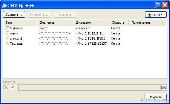
В диспетчере имён можно создать новые имена, просмотреть ранее созданные, и, при желании, изменить их.
Одно но: в диспетчере имён отображаются только видимые имена,
а в книге Excel могут присутствовать и скрытые.
Чтобы узнать количество имён в книге, а также посмотреть их значения,
мы воспользуемся макросом:
Sub ПолучениеСпискаИмёнВКниге()
    Dim n As Name, VisibleNames%, HiddenNames%, WB As Workbook, i As Long
    Set WB = ActiveWorkbook
    For Each n In WB.Names
        VisibleNames = VisibleNames - n.Visible
        HiddenNames = HiddenNames - Not n.Visible
    Next n

    If VisibleNames + HiddenNames = 0 Then
        MsgBox "Имена в книге отсутствуют (не назначены)", vbInformation
    Else
        msg = "Количество имён в книге: " & VisibleNames + HiddenNames & vbNewLine & _
              "Из них видимых: " & VisibleNames & ", скрытых: " & HiddenNames & vbNewLine & _
              vbNewLine & "Вывести на лист список всех имён?"
        If MsgBox(msg, vbInformation + vbYesNo, "Имена в открытом файле") = vbYes Then
            Dim sh As Worksheet: Set sh = Workbooks.Add(xlWBATWorksheet).Worksheets(1)
            sh.Cells(1, 1).Resize(, 4).Value = _
            Array("№", "Имя", "Видимость", "Ссылка (значение)")
            sh.Cells(1, 1).Resize(, 4).Interior.ColorIndex = 15
            For i = 1 To WB.Names.Count
                Set n = WB.Names(i)
                sh.Cells(i + 1, 1).Resize(, 4).Value = _
                Array(i, n.Name, IIf(n.Visible, "Видимое", "Скрытое"), "'" & n.RefersTo)
            Next i
            sh.UsedRange.EntireColumn.AutoFit
        End If
    End If
End Sub
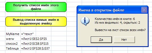
Для этого в прикреплённом файле нажмём зеленую кнопку,
и увидим вообщение с информацией о количестве имен в книге:
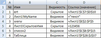
Если в диаоговом окне мы нажмём «Да», то макрос создаст новую книгу, и сформирует в ней таблицу со списком всех имен книги:
Если же вам требуется вывести список видимых имён на лист Excel, то можно воспользоваться макросом из одной строки:
Sub СписокВидимыхИмён()
    ActiveCell.ListNames
End Sub
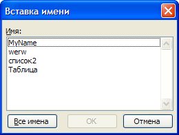
Того же эффекта можно добиться, нажав кнопку «Все имена» в диалоговом окне, вызываемом из меню Вставка — Имя — Вставить… (в Excel 2003):
- 29037 просмотров
Не получается применить макрос? Не удаётся изменить код под свои нужды?
Оформите заказ у нас на сайте, не забыв прикрепить примеры файлов, и описать, что и как должно работать.
VBA Listnames of Range Excel
VBA Listnames of range object will list the names in the workbook. It will list all the available named ranges and their corresponding definitions. If no names are defined in the workbook, it results nothing. This will be very useful if you have lot of named ranges in your workbook and see the all definitions at one glance. Particularly when you are moving the worksheets or deleting the worksheets, some of the named definitions will be corrupted(lost the refereces), In this case you can list all the available names in the workbook and see if they are missing any references.
VBA ListNames of Range – Syntax
Here is the syntax to find listnames in Excel range object. It will list all the available named ranges and their corresponding definitions.
Range(“YourRange”).ListNames
VBA ListNames of Range – Example
Below is the Excel VBA Macro or code to list all the available named ranges in the range “A1” and their corresponding definitions in the range “B1”
Sub Range_ListNaames()
    Range("A1").ListNames
End Sub
VBA ListNames of Range – Instructions
Please follow the below step by step instructions to execute the above mentioned VBA macros or codes:
- Open an Excel Workbook from your start menu or type Excel in your run command
- Add or define few names in your workbook to test the ListNames macro.
- Press Alt+F11 to Open VBA Editor or you can go to Developer Tab from Excel Ribbon and click on the Visual Basic Command to launch the VBA Editor
- Insert a Module from Insert Menu of VBA
- Copy the above code (for copying a range using VBA) and Paste in the code window(VBA Editor)
- Save the file as Macro Enabled Workbook (i.e; .xlsm file format)
- Press ‘F5′ to run it or Keep Pressing ‘F8′ to debug the code line by line.
Now, it will list all the available named ranges in the range “A1” and their corresponding definitions in the range “B1”. If no names are defined in the workbook, it results nothing. It is always a better practice to list the names in the workbook and check their definitions.
A Powerful & Multi-purpose Templates for project management. Now seamlessly manage your projects, tasks, meetings, presentations, teams, customers, stakeholders and time. This page describes all the amazing new features and options that come with our premium templates.
Save Up to 85% LIMITED TIME OFFER

All-in-One Pack
120+ Project Management Templates
Essential Pack
50+ Project Management Templates
Excel Pack
50+ Excel PM Templates
PowerPoint Pack
50+ Excel PM Templates
MS Word Pack
25+ Word PM Templates
Ultimate Project Management Template
Ultimate Resource Management Template
Project Portfolio Management Templates
VBA Reference
Effortlessly
Manage Your Projects
120+ Project Management Templates
Seamlessly manage your projects with our powerful & multi-purpose templates for project management.
120+ PM Templates Includes:
One Comment
-
John Christensen
April 25, 2016 at 7:47 AM — ReplyI’m confused – How is “B1” specified in the code example above? If I had this in the first row of a spreadsheet:
pi 3.1415
Then when I went to assign named ranges, the named range would be B1, not A1, right? The naming method (Alt-ShiftF4, if I remember) just uses the A1 cell to name the named range?
Isn’t Range(“A1”).ListNames just going to only look in A1, not A1 and B1?
thanks,
John
Effectively Manage Your
Projects and Resources
ANALYSISTABS.COM provides free and premium project management tools, templates and dashboards for effectively managing the projects and analyzing the data.
We’re a crew of professionals expertise in Excel VBA, Business Analysis, Project Management. We’re Sharing our map to Project success with innovative tools, templates, tutorials and tips.
Project Management
Excel VBA
Download Free Excel 2007, 2010, 2013 Add-in for Creating Innovative Dashboards, Tools for Data Mining, Analysis, Visualization. Learn VBA for MS Excel, Word, PowerPoint, Access, Outlook to develop applications for retail, insurance, banking, finance, telecom, healthcare domains.
Page load link
Go to Top
| title | keywords | f1_keywords | ms.prod | api_name | ms.assetid | ms.date | ms.localizationpriority |
|---|---|---|---|---|---|---|---|
|
Names object (Excel) |
vbaxl10.chm487072 |
vbaxl10.chm487072 |
excel |
Excel.Names |
ffecf89d-7bae-c470-8e37-608857a9de2a |
03/30/2019 |
medium |
Names object (Excel)
A collection of all the Name objects in the application or workbook.
Remarks
Each Name object represents a defined name for a range of cells. Names can be either built-in names—such as Database, Print_Area, and Auto_Open—or custom names.
The RefersTo argument must be specified in A1-style notation, including dollar signs ($) where appropriate. For example, if cell A10 is selected on Sheet1 and you define a name by using the RefersTo argument «=sheet1!A1:B1», the new name actually refers to cells A10:B10 (because you specified a relative reference). To specify an absolute reference, use «=sheet1!$A$1:$B$1».
Example
Use the Names property of the Workbook object to return the Names collection. The following example creates a list of all the names in the active workbook, plus the addresses that they refer to.
Set nms = ActiveWorkbook.Names
Set wks = Worksheets(1)
For r = 1 To nms.Count
    wks.Cells(r, 2).Value = nms(r).Name
    wks.Cells(r, 3).Value = nms(r).RefersToRange.Address
Next
Use the Add method to create a name and add it to the collection. The following example creates a new name that refers to cells A1:C20 on the worksheet named Sheet1.
Names.Add Name:="test", RefersTo:="=sheet1!$a$1:$c$20"
Use Names (index), where index is the name index number or defined name, to return a single Name object. The following example deletes the name mySortRange from the active workbook.
ActiveWorkbook.Names("mySortRange").Delete
This example uses a named range as the formula for data validation. This example requires the validation data to be on Sheet 2 in the range A2:A100. This validation data is used to validate data entered on Sheet1 in the range D2:D10.
Sub Add_Data_Validation_From_Other_Worksheet()
'The current Excel workbook and worksheet, a range to define the data to be validated, and the target range
'to place the data in.
Dim wbBook As Workbook
Dim wsTarget As Worksheet
Dim wsSource As Worksheet
Dim rnTarget As Range
Dim rnSource As Range

'Initialize the Excel objects and delete any artifacts from the last time the macro was run.
Set wbBook = ThisWorkbook
With wbBook
    Set wsSource = .Worksheets("Sheet2")
    Set wsTarget = .Worksheets("Sheet1")
    On Error Resume Next
    .Names("Source").Delete
    On Error GoTo 0
End With

'On the source worksheet, create a range in column A of up to 98 cells long, and name it "Source".
With wsSource
    .Range(.Range("A2"), .Range("A100").End(xlUp)).Name = "Source"
End With

'On the target worksheet, create a range 8 cells long in column D.
Set rnTarget = wsTarget.Range("D2:D10")

'Clear out any artifacts from previous macro runs, then set up the target range with the validation data.
With rnTarget
    .ClearContents
    With .Validation
        .Delete
        .Add Type:=xlValidateList, _
             AlertStyle:=xlValidAlertStop, _
             Formula1:="=Source"

'Set up the Error dialog with the appropriate title and message
        .ErrorTitle = "Value Error"
        .ErrorMessage = "You can only choose from the list."
    End With
End With

End Sub
Methods
- Add
- Item
Properties
- Application
- Count
- Creator
- Parent
See also
- Excel Object Model Reference
[!includeSupport and feedback]
As I promised last week, today’s tutorial is a dead easy macro that will allow you to extract a list of your worksheet tab names.
You can then use this list to:
- Create an index of your worksheets. Why not add Hyperlinks so you can quickly navigate your workbook.
- Or use them to create references on the fly with the INDIRECT function and much more.
Here’s how:
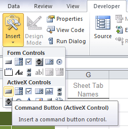
- Add a command button to the worksheet. Go to the Developer tab of the ribbon > Insert > Command Button from the ActiveX Controls group.
- Excel 2007 > Windows Button > Excel Options > Popular > Show Developer tab in the ribbon > OK.
- Excel 2010 > File tab > Options > Customize Ribbon > on the right hand window (Customize the Ribbon) tick the Developer box > OK.
- Draw the button on the worksheet. To re-size it click and drag the borders.
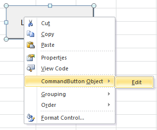
- Rename your command button. Right-click > CommandButton Object > Edit.
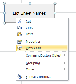
- Now, add Visual Basic code to the command button. Right-click > View Code:
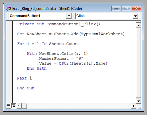
- In the Visual Basic Editor (VBA), enter the following code between the Private Sub CommandButton1_Click() statement and the End Sub statement:
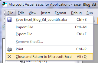
- On the File menu in the VBA editor, click Close and Return to Microsoft Excel.
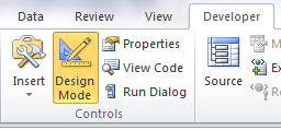
- Exit Design Mode by clicking on the Design Mode button on the Developer tab of the ribbon.
If you haven’t got the Developer Tab do the following:
Set NewSheet = Sheets.Add(Type:=xlWorksheet)

For i = 1 To Sheets.Count

    With NewSheet.Cells(i, 1)
        .NumberFormat = "@"
        .Value = CStr(Sheets(i).Name)
    End With

Next i
So it looks like this:
Now you’re ready to click the command button and watch the magic as Excel inserts a new sheet in your workbook with all of your sheet names listed and ready for action!
If you want to save the macro in your workbook you need to save the workbook as a ‘Macro Enabled Workbook’.
To do this go File > Save As > from the ‘Save as type’ list select ‘Excel Macro-Enabled Workbook (*.xlsm)’.

Whether your Microsoft Excel workbook has three sheets or 50, knowing what you have is important. Some complex applications require detailed documentation that includes sheet names. For those times when a quick look isn’t good enough, and you must have a list, you have a couple of options: You can go the manual route, which would be tedious and need updating every time you made a change. Or you can run a quick VBA procedure. In this article, I’ll show you easily modified code that generates a list of sheet names and hyperlinks. There are other ways to generate a list, but I prefer the VBA method because it’s automated and easy to modify to suit individual requirements.
SEE: 69 Excel tips every user should master (TechRepublic)
I’m using Microsoft 365 on a Windows 10 64-bit system, but you can use earlier versions. To save time, download the .xlsx, .xls and .cls files. Macros aren’t supported by the online version. This article assumes you have basic Excel skills and are familiar with VBA, but even a beginner should be able to follow the instructions to success.
How to enter and run code in VBA
If you’re new to VBA code, you might be wondering about the terms procedure and macro. You’ll see them used interchangeably when VBA is the language used. This isn’t true for all languages. In VBA, both a procedure and a macro are a named set of instructions that are preformed when called. Some developers refer to a sub procedure as a macro and a function procedure as a procedure because a procedure can accept arguments. Many use the term macro for everything. Some, like me, tend to use the term procedure for everything. Furthermore, Access has a macro feature that is separate from any VBA code. Don’t get too hung up on the terms.
SEE: Windows 10: Lists of vocal commands for speech recognition and dictation (free PDF) (TechRepublic)
To enter VBA code, press Alt + F11 to open the Visual Basic Editor. In the Project Explorer to the left, choose ThisWorkbook and enter the code. If you’re using a ribbon version, you must save the file as a macro-enabled file to use macros. You can also import the downloadable .cls file that contains the code. Or, you can work with either of the downloadable Excel workbooks. If you’re entering the code yourself, please don’t copy it from this web page. Instead, enter it manually or copy it to a text editor and then paste that code into a module.
When in the VBE, press F5 to run a procedure, but be sure to click inside the procedure you want to run. When in an Excel sheet, click the Developer tab, click Macros in the Code group, choose the procedure in the resulting dialog shown in Figure A, and then click Run.
Figure A

The bare bones VBA code
A simple list of sheet names is easy to generate using VBA thanks to the Worksheets collection. Listing A shows a simple For Each loop that cycles through this collection. For each sheet, the code uses the Name property to enter that name in column A, beginning at A1, in Sheet1.
Listing A
Sub ListSheetNames()
‘List all sheet names in column A of Sheet1.
‘Update to change location of list.
Sheets(“Sheet1”).Activate
ActiveSheet.Cells(1, 1).Select
‘Generate a list of hyperlinks to each sheet in workbook in Sheet1.
For Each sh In Worksheets
ActiveCell = sh.Name
ActiveCell.Offset(1, 0).Select ‘Move down a row.
Next
End Sub
When adapting this code, you might want to change the location of the list; do so by changing the first two lines accordingly. The For Each loop also offers possibilities for modifying. You might want to add header names or values to number the sheet names.
This code will list hidden and very hidden sheets, which you might not want. When that’s the case, you’ll need to check the Visible properties xlSheetVisible and xlSheetVeryHidden. In addition, because we’re actively selecting A1 on Sheet1, the cursor moves to that location. If you don’t want the active cell to change, use implicit selection statements. To learn more about implicit and explicit references, read Excel tips: How to select cells and ranges efficiently using VBA.
There are many modifications you might want to make. For example, instead of an ordinary list of text, you might want a list of hyperlinks.
How to generate a list of hyperlinks in Excel
It’s not unusual for a complex workbook to include a list of hyperlinks to each sheet in the workbook. The procedure you’ll use, shown in Listing B, is similar to Listing A, but this code uses the Name property to create a hyperlink.
Listing B
Sub ListSheetNamesAsHyperlinks()
‘Generate list of hyperlinks to each sheet in workbook in Sheet1, A1.
Sheets(“Sheet1”).Activate
ActiveSheet.Cells(1, 1).Select
‘Generate a list of hyperlinks to each sheet in workbook in Sheet1.
For Each sh In Worksheets
ActiveSheet.Hyperlinks.Add Anchor:=Selection, _
Address:=””, SubAddress:=”‘” & sh.Name & “‘” & “!A1”, _
TextToDisplay:=sh.Name
ActiveCell.Offset(1, 0).Select ‘Moves down a row
Next
End Sub
The first two lines select cell A1 in Sheet1. Update these two statements to relocate the list. The For Each loop cycles through all the sheets, using the Name property to create a hyperlink for each sheet.
The Hyperlinks.Add property in the For Each uses the form
.Add Anchor, Address, [SubAddress], [ScreenTip], [TextToDisplay]
The parameter information is listed below:
- Anchor: A Range or Shape object.
- Address: The address of the hyperlink.
- SubAddress: The subaddress of the hyperlink
- ScreenTip: Information displayed when the mouse pointer pauses over the hyperlink.
- TextToDisplay: The hyperlink text.
Our procedure’s SubAddress argument
SubAddress:=”‘” & sh.Name & “‘” & “!A1”
builds a string using the current sheet’s name and the cell reference A1. For instance, if the current sheet is Sheet1, this evaluates to ‘Sheet1’!A1. Subsequently, when you click this hyperlink, it takes you to cell A1 on Sheet1. As before, you can easily modify this procedure to reflect the way you want to use this list.
Both sub procedures are easy to use. Both can be easily modified to change the list’s position or to add more information to the simple list.