
Содержание
- Excel — Lock Range of Cells Based on Values
- 3 Answers 3
- Lock certain cells in a range
- 7 Answers 7
- How to lock a cell in Excel formula using VBA
- Protection
- Lock Cells
- Detect Cells with Formulas
- Lock cells and protect a worksheet
- Protecting cells in Excel but allow these to be modified by VBA script
- 6 Answers 6
- VBA protect and unprotect Sheets (25+ examples)
- Adapting the code for your purposes
- Protect and unprotect: basic examples
- Protect a sheet without a password
- Unprotect a sheet (no password)
- Protecting and unprotecting with a password
- VBA Protect sheet with password
- VBA Unprotect sheet with a password
- Using a password based on user input
- Catching errors when incorrect password entered
- Applying protection to different parts of the worksheet
- Protect contents
- Protect objects
- Protect scenarios
- Protect contents, objects and scenarios
- Applying protection to multiple sheets
- Protect all worksheets in the active workbook
- Protect the selected sheets in the active workbook
- Unprotect all sheets in active workbook
- Checking if a worksheet is protected
- Check if Sheet contents is protected
- Check if Sheet objects are protected
- Check if Sheet scenarios are protected
- Changing the locked or unlocked status of cells, objects and scenarios
- Lock a cell
- Lock all cells
- Lock a chart
- Lock a shape
- Lock a Scenario
- Allowing actions to be performed even when protected
- Allow sheet actions when protected
- Allow selection of any cells
- Allow selection of unlocked cells
- Don’t allow selection of any cells
- Allowing VBA code to make changes, even when protected
- Allowing the use of the Group and Ungroup feature
- Conclusion
Excel — Lock Range of Cells Based on Values
Is it possible to lock a particular range of cells based on the input from a dropdown in a row of data?
For example, each row of my spreadsheet represents a patient, and the first cell asks a question, to which a «Yes» or «No» response is required (which is selected/entered via a dropdown).
EDIT
The «Yes/No» cell is, in fact, a merge of two cells (G13 & H13). I have updated my example to reflect this.
EDIT ENDS
If the user selects «No», then I wish to lock the remainder of the range of questions (G13-H13:AB13) as there is no need to enter data here. However, if the user selects, «Yes», then the remainder of the cells shall remain available to enter data into.
All cells within each range have data entered via dropdowns only.
Here is what I am hoping to achieve:
Once again, I would like to emphasize that all data is entered via dropdown menus and that nothing is to be typed in manually; I would like it so that if G13-H13 = «No» , then the remainder of the cells within the range which have dropdowns are blocked or locked from having further information selected from their respective dropdowns.
Please note that the value in G13-H13 can be either «Yes» or «No».
Can this be achieved using VBA and if so, how?
3 Answers 3
EDIT: You can do this without VBA. I based this on another answer here: https://stackoverflow.com/a/11954076/138938
Column G has the Yes or No drop-down.
In cell H13, set up data validation like this:
- Data —> Data Validation
- Select List in the Allow drop-down.
- Enter this formula in the Source field: =IF($G13=»Yes», MyList, FALSE)
- Copy cell H13 and paste the validation (paste —> pastespecial —> validation) to cells I13:AB13.
- Replace MyList in the formula with the list you want to allow the user to select from for each column. Note that you’ll need to have the patient answer set to «Yes» in order to set up the validation. Once you set it up, you can delete it or set it to No.
- Once you have the validation set up for row 13, copy and paste the validation to all rows that need it.
If you want to use VBA, use the following, and use the worksheet_change event or some other mechanism to trigger the LockOrUnlockPatientCells. I don’t like using worksheet_change, but it may make sense in this case.
In order for the cells to be locked, you need to lock them and then protect the sheet. The code below does that. You need to pass it the row for the patient that is being worked on.
You can test the functionality by using the following, manually adjusting the values for the patient row. Once you get it to work the way you want, get the row from the user’s input.
Источник
Lock certain cells in a range
I’m trying to loop through a range of cells, locking any cell that has content while leaving empty cells unlocked.
When I run the below code the result is the entire sheet is locked. If I add an else statement the sheet is unlocked. Basically whatever the last .locked = (true, false) statement is is how the entire sheet winds up.
Change 1 Is it possible that I have some setting on/off that is interfering since I’m the only one who is unable to get any of this to work?
7 Answers 7

You can try this.

If you say Range(«A1»).Select, then it locks only A1. You can specify multiple cells to be locked by specifying as follows:
A3:A12,D3:E12,J1:R13,W18
This locks A3 to A12 and D3 to E12 etc.
I may be missing something but.
. will lock all cells on the active sheet. If you just change it to.
. then it works; I think?! As the range is very small, you may as well not unlock cells at the start, and instead unlock cells whilst locking them e.g.
If you are new to VBA, I would recommend cycling through code line-by-line as described in this Excel consultant’s video. If you step through code, you can check «has cell A7 behaved as expected?». instead of just seeing the end product
A quick way to unlock non-blank cells is to use SpecialCells see below.
On my testing this code handles merged cells ok, I think this is what is generating your error on Tim’s code when it looks to handle each cell individually (which to be clear is not an issue in Tim’s code, it is dealing with an unexpected outcome)
You may also find this article of mine A fast method for determining the unlocked cell range useful

I know this is an old thread, but I’ve been stuck on this for a while too, and after some testing on Excel 2013 here’s what I conclude if your range includes any merged cell
- The merged cells must be entirely included within that range (e.g. the merging must be entirely within the range being lock/unlocked
- The range being merged can be larger, or at least exactly the range corresponding to the merged cells. If it’s a named range that works as well.
Also, you cannot lock/unlock a cell that is already within a protected range. E.g if you run:
Twice it will work the first time, and fail the second time around. So you should unprotect the target range (or the sheet) before.
Источник
How to lock a cell in Excel formula using VBA

Users entering data into the wrong cells or changing existing formulas can make data collection a tedious process. However, you can prevent users from going outside the intended boundaries by disabling certain sections of your workbook. In this article, we’re going to show you how to lock a cell in Excel formula using VBA.
Protection
Worksheets are objects in a workbook’s worksheet collection and they have Protect and Unprotect methods. These methods determine the protected status of a worksheet as the name suggests. Both methods can get accept other optional arguments. The first is the password argument. By setting a string for the parameter argument, you can lock your worksheets with a password. Below is a breakdown.

Lock Cells
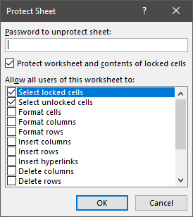
Important note: Protecting a sheet does not lock individual cells! The cells you want to lock should be marked as Locked too. A cell can be marked as Locked, and/or Hidden, in two ways:
The User Interface method requires using the Format Cells dialog. Select a cell or a range of cells, and press Ctrl + 1 to open this menu and go to the Protection tab. Use the corresponding checkboxes to activate properties.

The second method is doing this via VBA code. Every cell and range can be made Locked and FormulaHidden properties. Set these two as True or False to change their status.
You can use the Hidden status to hide your formulas as well.
Detect Cells with Formulas
If you just need to lock only cells with formulas, you need to first identify cells that have formulas. The cells and ranges have a HasFormula property, which makes them read only. It returns a Boolean value based on whether the cell or range has a formula. A simple loop can be used to detect cells in a given range that contain formula.
To run this code, you need to add a module into the workbook or the add-in file. Copy and paste the code into the module to run it. The main advantage of the module method is that it allows saving the code in the file, so that it can be used again later. Furthermore, the subroutines in modules can be used by icons in the menu ribbons or keyboard shortcuts. Remember to save your file in either XLSM or XLAM format to save your VBA code.
Lock cells and protect a worksheet
The code example below checks every cell in the range «B4:C9» from the active worksheet. If a cell has a formula, it locks the cell. Otherwise, the cell becomes or remains unlocked.
Источник
Protecting cells in Excel but allow these to be modified by VBA script
I am using Excel where certain fields are allowed for user input and other cells are to be protected. I have used Tools Protect sheet, however after doing this I am not able to change the values in the VBA script. I need to restrict the sheet to stop user input, at the same time allow the VBA code to change the cell values based on certain computations.

6 Answers 6
If the UserInterfaceOnly parameter is set to true, VBA code can modify protected cells.
Note however that this parameter does not stick. It needs to be reapplied each time the file is opened.
You can modify a sheet via code by taking these actions
In code this would be:
The weakness of this method is that if the code is interrupted and error handling does not capture it, the worksheet could be left in an unprotected state.
The code could be improved by taking these actions
The code to do this would be:
This code renews the protection on the worksheet, but with the ‘UserInterfaceOnly’ set to true. This allows VBA code to modify the worksheet, while keeping the worksheet protected from user input via the UI, even if execution is interrupted.
This setting is lost when the workbook is closed and re-opened. The worksheet protection is still maintained.
So the ‘Re-protection’ code needs to be included at the start of any procedure that attempts to modify the worksheet or can just be run once when the workbook is opened.
Источник
VBA protect and unprotect Sheets (25+ examples)

Protecting and unprotecting sheets is a common action for an Excel user. There is nothing worse than when somebody, who doesn’t know what they’re doing, overtypes essential formulas and cell values. It’s even worse when that person happens to be us; all it takes is one accidental keypress, and suddenly the entire worksheet is filled with errors. In this post, we explore using VBA to protect and unprotect sheets.
Protection is not foolproof but prevents accidental alteration by an unknowing user.
Sheet protection is particularly frustrating as it has to be applied one sheet at a time. If we only need to protect a single sheet, that’s fine. But if we have more than 5 sheets, it is going to take a while. This is why so many people turn to a VBA solution.
The VBA Code Snippets below show how to do most activities related to protecting and unprotecting sheets.
Download the example file: Click the link below to download the example file used for this post:
Adapting the code for your purposes
Unless stated otherwise, every example below is based on one specific worksheet. Each code includes Sheets(“Sheet1”)., this means the action will be applied to that specific sheet. For example, the following protects Sheet1.
But there are lots of ways to reference sheets for protecting or unprotecting. Therefore we can change the syntax to use one of the methods shown below.
Using the active sheet
The active sheet is whichever sheet is currently being used within the Excel window.
Applying a sheet to a variable
If we want to apply protection to a sheet stored as a variable, we could use the following.
Later in the post, we look at code examples to loop through each sheet and apply protection quickly.
Protect and unprotect: basic examples
Let’s begin with some simple examples to protect and unprotect sheets in Excel.
Protect a sheet without a password
Unprotect a sheet (no password)
Protecting and unprotecting with a password
Adding a password to give an extra layer of protection is easy enough with VBA. The password in these examples is hardcoded into the macro; this may not be the best for your scenario. It may be better to apply using a string variable, or capturing user passwords with an InputBox.
VBA Protect sheet with password
VBA Unprotect sheet with a password
NOTE – It is not necessary to unprotect, then re-protect a sheet to change the settings. Instead, just protect again with the new settings.
Using a password based on user input
Using a password that is included in the code may partly defeat the benefit of having a password. Therefore, the codes in this section provide examples of using VBA to protect and unprotect based on user input. In both scenarios, clicking Cancel is equivalent to entering no password.
Protect with a user-input password
Unprotect with a user-input password
Catching errors when incorrect password entered
If an incorrect password is provided, the following error message displays.
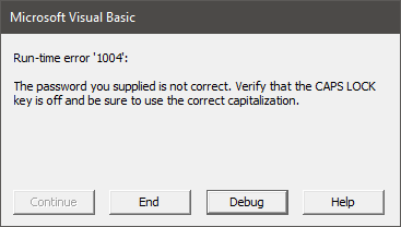
The code below catches the error and provides a custom message.
If you forget a password, don’t worry, the protection is easy to remove.
Applying protection to different parts of the worksheet
VBA provides the ability to protect 3 aspects of the worksheet:
- Contents – what you see on the grid
- Objects – the shapes and charts which are on the face of the grid
- Scenarios – the scenarios contained in the What If Analysis section of the Ribbon
By default, the standard protect feature will apply all three types of protection at the same time. However, we can be specific about which elements of the worksheet are protected.
Protect contents
Protect objects
Protect scenarios
Protect contents, objects and scenarios
Applying protection to multiple sheets
As we have seen, protection is applied one sheet at a time. Therefore, looping is an excellent way to apply settings to a lot of sheets quickly. The examples in this section don’t just apply to Sheet1, as the previous examples have, but include all worksheets or all selected worksheets.
Protect all worksheets in the active workbook
Protect the selected sheets in the active workbook
Unprotect all sheets in active workbook
Checking if a worksheet is protected
The codes in this section check if each type of protection has been applied.
Check if Sheet contents is protected
Check if Sheet objects are protected
Check if Sheet scenarios are protected
Changing the locked or unlocked status of cells, objects and scenarios
When a sheet is protected, unlocked items can still be edited. The following codes demonstrate how to lock and unlock ranges, cells, charts, shapes and scenarios.
When the sheet is unprotected, the lock setting has no impact. Each object becomes locked on protection.
All the examples in this section set each object/item to lock when protected. To set as unlocked, change the value to False.
Lock a cell
Lock all cells
Lock a chart
Lock a shape
Lock a Scenario
Allowing actions to be performed even when protected
Even when protected, we can allow specific operations, such as inserting rows, formatting cells, sorting, etc. These are the same options as found when manually protecting the sheet.
Allow sheet actions when protected
Allow selection of any cells
Allow selection of unlocked cells
Don’t allow selection of any cells
Allowing VBA code to make changes, even when protected
Even when protected, we still want our macros to make changes to the sheet. The following VBA code changes the setting to allow macros to make changes to a protected sheet.
Unfortunately, this setting is not saved within the workbook. It needs to be run every time the workbook opens. Therefore, calling the code in the Workbook_Open event of the Workbook module is probably the best option.
Allowing the use of the Group and Ungroup feature
To enable users to make use of the Group and Ungroup feature of protected sheets, we need to allow changes to the user interface and enable outlining.
As noted above the UserInterfaceOnly setting is not stored in the workbook; therefore, it needs to be run every time the workbook opens.
Conclusion
Wow! That was a lot of code examples; hopefully, this covers everything you would ever need for using VBA to protect and unprotect sheets.
Related posts:

About the author
Hey, I’m Mark, and I run Excel Off The Grid.
My parents tell me that at the age of 7 I declared I was going to become a qualified accountant. I was either psychic or had no imagination, as that is exactly what happened. However, it wasn’t until I was 35 that my journey really began.
In 2015, I started a new job, for which I was regularly working after 10pm. As a result, I rarely saw my children during the week. So, I started searching for the secrets to automating Excel. I discovered that by building a small number of simple tools, I could combine them together in different ways to automate nearly all my regular tasks. This meant I could work less hours (and I got pay raises!). Today, I teach these techniques to other professionals in our training program so they too can spend less time at work (and more time with their children and doing the things they love).
Do you need help adapting this post to your needs?
I’m guessing the examples in this post don’t exactly match your situation. We all use Excel differently, so it’s impossible to write a post that will meet everybody’s needs. By taking the time to understand the techniques and principles in this post (and elsewhere on this site), you should be able to adapt it to your needs.
But, if you’re still struggling you should:
- Read other blogs, or watch YouTube videos on the same topic. You will benefit much more by discovering your own solutions.
- Ask the ‘Excel Ninja’ in your office. It’s amazing what things other people know.
- Ask a question in a forum like Mr Excel, or the Microsoft Answers Community. Remember, the people on these forums are generally giving their time for free. So take care to craft your question, make sure it’s clear and concise. List all the things you’ve tried, and provide screenshots, code segments and example workbooks.
- Use Excel Rescue, who are my consultancy partner. They help by providing solutions to smaller Excel problems.
What next?
Don’t go yet, there is plenty more to learn on Excel Off The Grid. Check out the latest posts:
Источник
The case – you have a multi-sheet Excel file, where you need to lock each cell in a given sheet. You have an option to do it manually, but it takes time and you need twice the time to check later. Or you may use VBA and be happy about it.

The choice is yours 🙂
Here is what the VBA does:
- Selects each sheet in the file.
- Checks whether its name is different from “SomeSheetName“
- Activates the sheet
- Locks range C1 and A1:A40.
- Sets a password “vitoshacademy” for it.
Once this is done, you are a happy owner of a well locked sheet. If you want to unlock it, again you have two options. Option A – to do it manually and then to lose time for checking it sheet by sheet and option B – to use 8 lines of VBA code. It’s your choice, but if you want to use the VBA, here comes the code:
|
Sub <span class=«hiddenSpellError»>UnlockAll</span>() Dim sheet As Worksheet For Each sheet In ThisWorkbook.Worksheets sheet.Activate ActiveSheet.Unprotect Password:=«<span class=»hiddenSpellError«>vitoshacademy</span>» ActiveSheet.Cells.Locked = False Next sheet End Sub |
And here is the code for the first example:
|
Sub <span class=«hiddenSpellError»>LockSomething</span>() Dim sheet As Worksheet For Each sheet In ThisWorkbook.Worksheets If (sheet.Name <> «<span class=»hiddenSpellError«>SomeSheetName</span>») And (sheet.Name <> «<span class=»hiddenSpellError«>OtherSheetName</span>») Then Debug.Print sheet.Name sheet.Activate Range(«<span class=»hiddenSpellError«>C1</span>»).Locked = True Range(«A1:<span class=»hiddenSpellError«>A40</span>»).Locked = True ActiveSheet.Protect Password:=«<span class=»hiddenSpellError«>vitoshacademy</span>» End If Next sheet End Sub |
🙂
In this post, I am going to show you how to lock and unlock cells using Conditional Formatting and VBA.
Why did I need this?
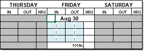
One of the improvements for the Student_Timesheet_Tool.xlsm was to prevent data entry in dates that were not in the selected period. The previous file allowed data entry in every cell; it was even possible to delete formulas. This was a feature that I knew I wanted to address.
The Goal
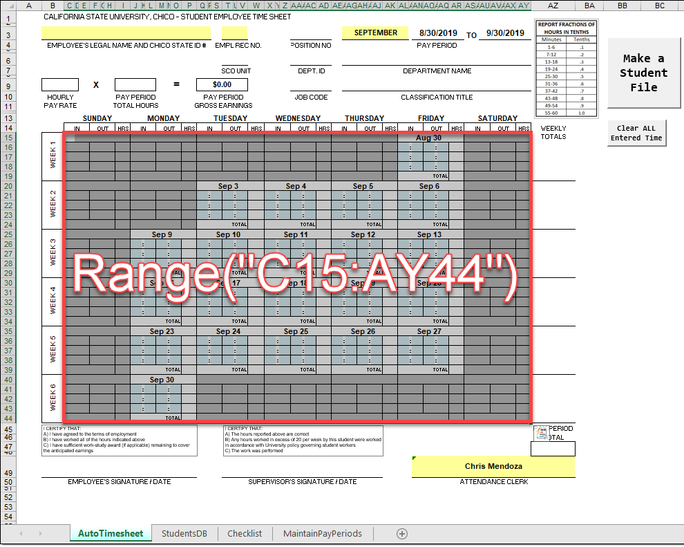
The new improved file would only allow users to enter/modify data in the cells which I allow. The dynamic nature of this feature is actually pretty in depth but, I will show the foundation for the solution.
Setting the base background color
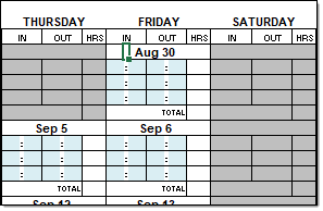
In the calendar matrix, data entry should only occur in cells designated either ‘IN’ or ‘OUT’. For each of those cells, I decided to fill them in Aqua.
Not only are each of these named ranges filled Aqua, they are also unlocked in Format Cells > Protection.
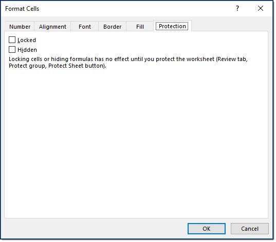
Every other cell in the worksheet that is not Yellow or Aqua is ‘Locked’ in Format Cells > Protection.
VBA Code
Visually filling the cells Aqua, or some other color, actually has a really important role in this locking and unlocking of cells. Without the color, how would you tell Excel which cells need to be locked and unlocked? This is how I told Excel what to do.
Public Sub LockCells()
    currentSheetName = ActiveSheet.Name
    Dim rng As Range: Set rng = Worksheets(currentSheetName).Range("C15:AY44")
    Dim cel As Range

    'colorIndex = 15 - White, Background 1, Darker 25%
    'colorIndex = 20 - Aqua, Accent 5, Lighter 80%

    Worksheets(currentSheetName).Unprotect Password:="SuperSecretPassword"
    For Each cel In rng.Cells
        With cel
            If .DisplayFormat.Interior.colorIndex = 15 Then
                .Locked = True
            ElseIf .DisplayFormat.Interior.colorIndex = 20 Then
                .Locked = False
            End If
        End With
    Next cel
    Worksheets(currentSheetName).Protect Password:="SuperSecretPassword", userinterfaceonly:=True
End Sub
colorIndex = 15 is the Gray and colorIndex = 20 is the Aqua color. So the base color is always Aqua and the Gray color comes from plain old conditional formatting that I’ll talk about in a bit. The .Locked = true is the same as you checking the box in the Format Cells dialog.
Conditional Formatting
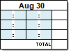
Before we can talk about the Conditional Formatting rules I have to explain a little bit about how the dates are generated/displayed. Using the period ‘SEPTEMBER’ as an example:
=IF(
  $AN$1="**********",
  IF(
    AF15="**********",
    IF(
      WEEKDAY($AN$3)=6,
      $AN$3,
      "**********"
    ),
    AF15+1
  ),
  IF(
    WEEKDAY($AN$1)=6,
    $AN$1,
    AF15+1
  )
)
Basically, our need for understanding in this post is, is this value an integer. If it is, we do something, if it is not, we do something else.
So let’s find out if what is returned is an integer or not.
If AM15 is a number, return 1, otherwise 0. Remember a date is an integer. Incidentally, you’re not seeing either the 1 or 0 because I have changed the font color to white.
Ok, now the Conditional Formatting
For each date range I wrote conditional formatting to check whether or not a 1 or 0 exists.

Can you see how that works?
The Result
The Sub LockCells () gets called in a Private Sub Worksheet_Change () event, the drop down selection change making the locking and unlocking of cells dynamic.
- Remove From My Forums
-
Question
-
Dear All !! I have one Excel 2010 File. I want some Ranges and some indivisual cells as ReadOnly but rest of the file should remain editable. These read ReadOnly Ranges & cells should hide the formula as well, as I want the result
should be displayed but not the formula. I have done that one through Excel Menu Command but it does not match with my requirement. Following are the details of the Colum, Rows & Cells which required VBA Codes for the above actions:Row
90 Cell K98Cell
C133 Cell
C135Column Range……. C95:C125 Column
Range…… D96:D125Column Range…… G95:G125 Column
Range…… H95:H125Column Range…… H130:H131 Column
Range…… H133:H135Thanks!………… Kahn-Cann
Answers
-
http://stackoverflow.com/questions/3037400/how-to-lock-the-data-in-a-cell-in-excel-using-vba
this worked for me.
Please do not forget to click “Vote as Helpful” if the reply helps/directs you toward your solution and or «Mark as Answer» if it solves your question. This will help to contribute to the forum.
-
Marked as answer by
Monday, October 1, 2012 2:59 AM
-
Marked as answer by
-
#3
Sorry, changed something
Link HERE
D I C K .
-
#4
Sorry, changed something
Link HERE
D I C K .
Hello ****,
Thank you for your response, but i am unable to retrive the file you have mentioned using the above mentioned link, can you please send me the macro code?
-
#5
This code should be located in the codepart of sheet1
NOT in a module
put anything in te cells a1 and a2
when you change to sheet2 and then back, see what happens.
To reset click Alt-F8 and execute RESET
****.
Code:
Sub LockColumns()
Application.ScreenUpdating = True
With Application.Sheets(1)
    .Unprotect
    .Activate
    .Cells(1, 1).Select
    Do While Selection.Value <> ""                         'If selection is not empty
            Selection.EntireColumn.Interior.Color = 65535
            Selection.EntireColumn.Locked = True
            Selection.Offset(0, 1).Select
    Loop
    .Protect DrawingObjects:=True, Contents:=True, Scenarios:=True
End With
End Sub


Sub Reset()
    Sheets("Blad1").Select
    Sheets("Blad1").Unprotect
    Cells.Select
    With Selection.Interior
        .Pattern = xlNone
        .TintAndShade = 0
        .PatternTintAndShade = 0
    End With
    Selection.Locked = False
    Selection.FormulaHidden = False
    With Selection.Interior
        .Pattern = xlNone
        .TintAndShade = 0
        .PatternTintAndShade = 0
    End With
    Sheets("Blad1").Range("A1").Select
End Sub


Private Sub Worksheet_Activate()
    LockColumns
End Sub
Last edited: Oct 15, 2014
-
#6
This code should be located in the codepart of sheet1
NOT in a moduleput anything in te cells a1 and a2
when you change to sheet2 and then back, see what happens.
To reset click Alt-F8 and execute RESET
****.
Code:
Sub LockColumns()
Application.ScreenUpdating = True
With Application.Sheets(1)
    .Unprotect
    .Activate
    .Cells(1, 1).Select
    Do While Selection.Value <> ""                         'If selection is not empty
            Selection.EntireColumn.Interior.Color = 65535
            Selection.EntireColumn.Locked = True
            Selection.Offset(0, 1).Select
    Loop
    .Protect DrawingObjects:=True, Contents:=True, Scenarios:=True
End With
End Sub


Sub Reset()
    Sheets("Blad1").Select
    Sheets("Blad1").Unprotect
    Cells.Select
    With Selection.Interior
        .Pattern = xlNone
        .TintAndShade = 0
        .PatternTintAndShade = 0
    End With
    Selection.Locked = False
    Selection.FormulaHidden = False
    With Selection.Interior
        .Pattern = xlNone
        .TintAndShade = 0
        .PatternTintAndShade = 0
    End With
    Sheets("Blad1").Range("A1").Select
End Sub


Private Sub Worksheet_Activate()
    LockColumns
End Sub
_—————————————————————————————————
Hello ****,
I tried the above code, but it is coloring the whole sheet 1, but not the cells with data. And i want to present my problem more clearly….As below
1. As i opens this sheet every time the data from Row # 2 to the last row containg the data must locked. (In this case- From teh row 2 to row 4 has to be locked).
2.Row1 will always be empty, bcas i need to enter the data in that row and click on «Add data» command button. Then teh data will be added at the last empty available empty row in teh sheet. In teh below i have entered teh new data «Walsh, 111» and click on the Add data button teh data will be added in the last empty row.
Before adding the data
| Walsh | 111 | Add Data | |
| Name | Number | ||
| Hari | 11 | ||
| Raj | 99 | ||
<COLGROUP><COL style=»WIDTH: 48pt» span=4 width=64><TBODY>
</TBODY>
AFter Adding the Data
| Add Data | |||
| Name | Number | ||
| Hari | 11 | ||
| Raj | 99 | ||
| Walsh | 111 |
<COLGROUP><COL style=»WIDTH: 48pt» span=4 width=64><TBODY>
</TBODY>
3. Now the data from Row 2 to row that contains the data i.e. Row # 5 has to be locked. I mean only the cells with data has to be locked always, even every time when i opens the sheet. (I mean immedietly when i opens the work sheet/workbook the data from Row to last row containing data has to be locked)…
I have macro now for adding the data at the bottom , but i need to have a macro only for locking the cells that contains the data always and that macro need to lock all the available data from row #2)
And if I want to edit any changes in the data from row # 2 it should ask me for a password.
Regards
Harikrishna
-
#7
Hello Harikrishna,
I think it’s more logical to protect the data that has been entered right away.
When your macro has done it’s job to put the data at the bottom of the table you can use the code below to protect the first and second column of the rows that have been filled.
The First column changes to and has to be protected also.
The cells containing Name and Number have to be named accordingly. The code will determine the range by starting with the cell under the named range (Name) and extend it to the last continuously filled cells below and then protect it.
So Everything stays protected until your code, including mine, will change the sheet and the protection. The only cells affected by the code are the cells below Name and Number. The rest of your protected and unprotected cells will keep unchanged.
Code:
Sub LockRange()
    With Application.Sheets(1)
        .Unprotect Password:="Password"
        Range(Range("Name").Offset(0, 1), Selection.End(xlDown)).Locked = True
        Range(Range("Number").Offset(0, 1), Selection.End(xlDown)).Locked = True
        .Protect Password:="Password"
    End With
End Sub
The columns cannot have blanks because the xlenddown will not work, but your code prevents this from happening.
When you rightclick the tab to unprotect your sheet you will have to enter the same password that is in the code. This enables you to edit any cell in the sheet. Do not forget to protect the sheet before saving.
You will have to protect your code for opening by a password because everyone, able to type Alt-F11 will be able to read your password in de code that is used.
Well, it was interesting to figure this out. I hope it helps. And do not forget the most important feature in the VBA editor being F1, the mother of all your answers.
Hope to read your reaction to this all.
D I C K .
-
#8
Sorry still al little mistake in the code.
Corrected below
Code:
Sub LockRange()
    With Application.Sheets(1)
        .Unprotect Password:="Password"
        Range(Range("Name").Offset(1, 0), Range("Name").Offset(1, 0).End(xlDown)).Locked = True
        Range(Range("Number").Offset(1, 0), Range("Number").Offset(1, 0).End(xlDown)).Locked = True
        .Protect Password:="Password"
    End With
End Sub