
Определение блока ячеек, расположенного на пересечении двух и более диапазонов, с помощью метода Application.Intersect из кода VBA Excel. Пример.
Описание
Application.Intersect – это метод VBA Excel, возвращающий прямоугольный объект Range, находящийся на пересечении двух или более указанных диапазонов.
Если общие ячейки для всех заданных диапазонов не обнаружены, метод Application.Intersect возвращает значение Nothing.
Если в качестве аргументов метода Application.Intersect указаны диапазоны из разных листов, возвращается ошибка.
Синтаксис
|
Application.Intersect (Arg1, Arg2, Arg3, ..., Arg30) |
- Arg1, Arg2 – обязательные аргументы, представляющие из себя пересекающиеся диапазоны (объекты Range).
- Arg3, …, Arg30* – необязательные аргументы, представляющие из себя пересекающиеся диапазоны (объекты Range).
* Допустимо использование до 30 аргументов включительно.
Пример
|
Sub Primer() Dim rngis As Range, arg1 As Range, arg2 As Range, arg3 As Range Set arg1 = Range(«A1:F10») Set arg2 = Range(«C4:I18») Set arg3 = Range(«D1:F22») Set rngis = Application.Intersect(arg1, arg2, arg3) If rngis Is Nothing Then MsgBox «Указанные диапазоны не пересекаются» Else MsgBox «Адрес пересечения диапазонов: « & rngis.Address End If End Sub |
Строку
|
Set rngis = Application.Intersect(arg1, arg2, arg3) |
можно записать без использования переменных так:
|
Set rngis = Application.Intersect(Range(«A1:F10»), Range(«C4:I18»), Range(«D1:F22»)) |
Есть и другой способ определения пересечения диапазонов. Он заключается в использовании свойства Range объекта Worksheet*:
|
Set rngis = Range(«A1:F10 C4:I18 D1:F22») ‘или Set rngis = Range(arg1.Address & » « & arg2.Address & » « & arg3.Address) |
Но у этого способа есть существенных недостаток – свойство Range возвращает ошибку, если пересечение указанных диапазонов не существует. Поэтому преимущество остается за методом Application.Intersect, который, в этом случае, возвратит значение Nothing.
* Если код VBA Excel работает со свойствами активного листа, объект Worksheet можно не указывать. Например, строка MsgBox Name отобразит имя активного листа.
|
Прошу помочь разобраться в макросе с Target и Intersect |
||||||||
Ответить |
||||||||
Ответить |
||||||||
Ответить |
||||||||
Ответить |
||||||||
Ответить |
||||||||
Ответить |
||||||||
Ответить |
||||||||
Ответить |
||||||||
Ответить |
||||||||
Ответить |
||||||||
Ответить |
||||||||
Ответить |
||||||||
Ответить |
||||||||
Ответить |
||||||||
Ответить |
||||||||
Ответить |
||||||||
Ответить |
||||||||
Ответить |
||||||||
Ответить |
||||||||
Ответить |


Return to VBA Code Examples
In this Article
- Union
- Intersect
- Use of Intersect
Excel VBA has two methods, belonging to Application object, to manipulate two or more ranges: Union and Intersect.
Union
Union method returns all the cells in two or more ranges passed as its argument.
The following command will select the range shown in the image below:
Union(Range("A1:B4"),Range("B3:C6")).Select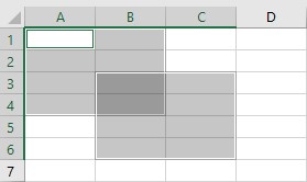
You can assign any value or formula to the range returned by the Union method:
Union(Range("A1:B4"), Range("B3:C6")) = 10This will enter the value 10 in each cell in the Union.
You can wrap any function which summarizes a range around an Union method. Following example will return the sum of the values in the Ranges A1:B4 and B3:C6:
Result = Application.WorksheetFunction.Sum(union(Range("A1:B4"), Range("B3:C6")))You might be surprised to get the value in Result as 160! Although there are only 14 cells in the Union (8 in each range with 2 being common) when you look at Selection, Union actually returns 16 cells hence the Result as 160.
Intersect
Intersect method returns only the common cells in two or more ranges passed as its argument.
The following command will select the range shown (Gray area) in the image below:
Intersect(Range("A1:B4"),Range("B3:C6")).Select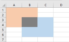
Use of Intersect
The most common usage of Intersect is in events associated with a Worksheet or Workbook. It is used to test whether the cell(s) changed belong to a a range of interest. Following example with check whether the cell(s) changed (identified by Target) and Range A1:A10 are common and take appropriate action if they are.
Intersect object returns nothing if there are no common cells so Intersect(Target, Range(“A1:A10”)) Is Nothing will be True if there are no common cells. Adding Not to the condition makes it True only if the result of the test Intersect(Target, Range(“A1:A10”)) Is Nothing is False, in other words Target and Range A1:A10 have some cells in common.
Private Sub Worksheet_Change(ByVal Target As Range)
	If Not Intersect(Target, Range("A1:A10")) Is Nothing Then
		' Take desired action
	End If
End Sub
Written by: Vinamra Chandra
VBA Coding Made Easy
Stop searching for VBA code online. Learn more about AutoMacro — A VBA Code Builder that allows beginners to code procedures from scratch with minimal coding knowledge and with many time-saving features for all users!

Learn More!
Excel VBA Refer to Ranges — Union & Intersect; Resize; Areas, CurrentRegion, UsedRange & End Properties; SpecialCells
An important aspect in vba coding is referencing and using Ranges within a Worksheet. You can refer to or access a worksheet range using properties and methods of the Range object. A Range Object refers to a cell or a range of cells. It can be a row, a column or a selection of cells comprising of one or more rectangular / contiguous blocks of cells. This section (divided into 2 parts) covers various properties and methods for referencing, accessing & using ranges, divided under the following chapters:
Excel VBA Referencing Ranges — Range, Cells, Item, Rows & Columns Properties; Offset; ActiveCell; Selection; Insert:
Range Property, Cells / Item / Rows / Columns Properties, Offset & Relative Referencing, Cell Address;
Activate & Select Cells; the ActiveCell & Selection;
Entire Row & Entire Column Properties, Inserting Cells/Rows/Columns using the Insert Method;
Excel VBA Refer to Ranges — Union & Intersect; Resize; Areas, CurrentRegion, UsedRange & End Properties; SpecialCells:
Ranges — Union & Intersect;
Resize a Range;
Referencing — Contiguous Block(s) of Cells, Range of Contiguous Data, Cells Meeting a Specified Criteria, Used Range, Cell at the End of a Block / Region, Last Used Row or Column;
Related Links:
Working with Objects in Excel VBA
Excel VBA Application Object, the Default Object in Excel
Excel VBA Workbook Object, working with Workbooks in Excel
Microsoft Excel VBA — Worksheets
Excel VBA Custom Classes and Objects
———————————————————————————————————
Contents:
Ranges — Union & Intersect
Resize a Range
Referencing — Contiguous Block(s) of Cells, Range of Contiguous Data, Cells Meeting a Specified Criteria, Used Range, Cell at the End of a Block / Region, Last Used Row or Column
———————————————————————————————————
Ranges — Union & Intersect
Use the Application.Union Method to return a range object representing a union of two or more range objects. Syntax: ApplicationObject.Union(Arg1, Arg2, … Arg29, Arg30). Each argument is a range object and it is necessary to specify atleast 2 range objects as arguments.
Using the union method set the background color of cells B1 & D3 in Sheet1 to red:
Union(Worksheets(«Sheet1»).Cells(1, 2), Worksheets(«Sheet1»).Cells(3, 4)).Interior.Color = vbRed
Using the union method set the background color of 2 named ranges to red:
Union(Range(«NamedRange1»), Range(«NamedRange2»)).Interior.Color = vbRed
Example 8: Using the Union method:
Sub RangeUnion()
Dim rng1 As Range, rng2 As Range, rngUnion As Range
Set rng1 = ActiveWorkbook.Worksheets(«Sheet3»).
Range(«A2:B3»)
Set rng2 = ActiveWorkbook.Worksheets(«Sheet3»).
Range(«C5:D7»)
‘using the union method:
Set rngUnion = Union(rng1, rng2)
‘this will set the background color to red, of cells A2, A3, B2, B3, C5, C6, C7, D5, D6 & D7 in Sheet3 of active workbook:
rngUnion.Interior.Color = vbRed
End Sub
Determining a range which is at the intersection of multiple ranges is a useful tool in vba programming, and is also often used to determine whether the changed range is within or is a part of the specified range in the context of Excel built-in Worksheet_Change Event, wherein a VBA procedure or code gets executed when content of a worksheet cell changes. Using the Application.Intersect Method returns a Range which is at the intersection of two or more ranges. Syntax: ApplicationObject.Intersect(Arg1, Arg2, Arg3, … Arg 30). Specifying the Application object qualifier is optional. Each argument represents the intersecting range and a minimum of two ranges are required to be specified. Refer below examples which explain useing the Intersect method, and also using it in combination with the Union method.
Example 9: Using the Intersect method.
Sub IntersectMethod()
‘examples of using Intersect method
Dim ws As Worksheet
Set ws = Worksheets(«Sheet2»)
‘note that the active cell (used below) can be referred to only in respect of the active worksheet:
ws.Activate
‘—————-
‘If the active cell is within the specified range of A1:B5, its background color will be set to red, however if the active cell is not within the specified range of A1:B5, say the active cell is A10, then you will get a run time error. You can check whether the active cell is within the specified range, as shown below where an If…Then statement is used.
Intersect(ActiveCell, Range(«A1:B5»)).Interior.Color = vbRed
‘—————-
‘If the active cell is not within the specified range of A1:B5, say the active cell is A10, then you will get a run time error. You can check whether the active cell is within the specified range, as shown below where an
If…Then statement is used.
If Intersect(ActiveCell, Range(«A1:B5»)) Is Nothing Then
‘if the active cell is not within the specified range of A1:B5, say the active cell is A10, then below message is returned:
MsgBox «Active Cell does not intersect»
Else
‘if the active cell is within the specified range of A1:B5, say the active cell is A4, then the address «$A$4» will be returned below:
MsgBox Intersect(ActiveCell, Range(«A1:B5»)).Address
‘—————-
‘consider 2 named ranges: «NamedRange8» comprising of range C1:C8 and «NamedRange9» comprising of range A5:E6:
If Intersect(Range(«NamedRange8»), Range(«NamedRange9»)) Is Nothing Then
‘if the ranges do not intersect, then below message will be returned:
MsgBox «Named Ranges do not intersect»
Else
‘in this case, the 2 named ranges intersect, hence the background color of green will be applied to the intersected range of C5:C6:
Intersect(Range(«NamedRange8»), Range(«NamedRange9»)).Interior.Color = vbGreen
End If
End Sub
Example 10: Using Intersect and Union methods in combination — refer Images 6a, 6b, 6c & 6d.
For live code of this example, click to download excel file.
Sub IntersectUnionMethods()
‘using Intersect and Union methods in combination — refer Images 6a, 6b, 6c & 6d.
Dim ws As Worksheet
Dim rng1 As Range, rng2 As Range, cell As Range, rngFinal1 As Range, rngUnion As Range, rngIntersect As Range, rngFinal2 As Range
Dim count As Integer
Set ws = Worksheets(«Sheet1»)
‘set ranges:
Set rng1 = ws.Range(«B1:C10»)
Set rng2 = ws.Range(«A5:D7»)
‘we work on 4 options: (1) cells in rng1 plus cells in rng2; (2) cells common to both rng1 & rng2; (3) cells in rng1 but not in rng2 ie. exclude intersect range from rng1; (4) cells not common to both rng1 & rng2. The first 2 options simply use the Union and Intersect methods respectively. See below.
‘NOTE: each of the 4 below codes need to be run individually.
‘clear background color in worksheet before starting code:
ws.Cells.Interior.ColorIndex = xlNone
‘—————-
‘(1) cells in rng1 plus cells in rng2 — using the Union method, set the background color to red (refer Image 6a):
Union(rng1, rng2).Interior.Color = vbRed
‘—————-
‘(2) cells common to both rng1 & rng2 — using the Intersect method, set the background color to red, of range B5:C7 (refer Image 6b):
If Intersect(rng1, rng2) Is Nothing Then
MsgBox «Ranges do not intersect»
Else
Intersect(rng1, rng2).Interior.Color = vbRed
End If
‘—————-
‘(3) cells in rng1 but not in rng2 ie. exclude intersect range from rng1 — set the background color to red (refer Image 6c):
count = 0
‘check each cell of rng1, and exclude it from final range if it is a part of the intersect range:
For Each cell In rng1
If Intersect(cell, rng2) Is Nothing Then
count = count + 1
‘determine first cell for the final range:
‘instead of «If count = 1 Then» you can alternatively use: «If rngFinal1 Is Nothing Then»
If count = 1 Then
‘include a single (ie. first) cell in the final range:
Set rngFinal1 = cell
Else
‘set final range as union of further matching cells:
Set rngFinal1 = Union(rngFinal1, cell)
End If
End If
Next
rngFinal1.Interior.Color = vbRed
‘—————-
‘(4) cells not common to both rng1 & rng2 ie. exclude intersect area from their union — set the background color to red (refer Image 6d):
Set rngUnion = Union(rng1, rng2)
‘check if intersect range is not empty:
If Not Intersect(rng1, rng2) Is Nothing Then
Set rngIntersect = Intersect(rng1, rng2)
‘check for each cell in the union of both ranges, whether it is also a part of their intersection:
For Each cell In rngUnion
‘if a cell is not part of the intersection of both ranges, then include in the final range:
If Intersect(cell, rngIntersect) Is Nothing Then
‘the first eligible cell for the final range:
If rngFinal2 Is Nothing Then
Set rngFinal2 = cell
Else
Set rngFinal2 = Union(rngFinal2, cell)
End If
End If
Next
‘apply color to the unuion of both ranges excluding their intersect area:
rngFinal2.Interior.Color = vbRed
‘if intersect range is empty:
Else
‘apply color to the union of both ranges if no intersect area:
rngUnion.Interior.Color = vbRed
End If
End Sub
The Intersect method is commonly used with the Excel built-in Worksheet_Change Event (or with the Worksheet_SelectionChange event). You can auto run a VBA code, when content of a worksheet cell changes, with the Worksheet_Change event. The change event occurs when cells on the worksheet are changed. The Intersect method is used to determine whether the changed range is within or is a part of the defined range in this context. Target is a parameter or variable of data type Range ie. Target is a Range Object. It refers to the changed Range and can consist of one or multiple cells. If Target is in the defined Range, and its value or content changes, it will trigger the vba procedure. If Target is not in the defined Range, nothing will happen in the worksheet. The Intersect method is used to determine whether the Target or changed range lies within (or intersects) with the defined range. Note that Worksheet change procedure is installed with the worksheet ie. it must be placed in the code module of the appropriate Sheet object (in the VBE Code window, select «Worksheet» from the left-side «General» drop-down menu and then select «Change» from the right-side «Declarations» drop-down menu). Refer below examples.
Examples of using Intersect method with the worksheet change or selection change events:
Private Sub Worksheet_Change(ByVal Target As Range)
‘Worksheet change procedure is installed with a worksheet ie. it must be placed in the code module of the appropriate Sheet object
‘using Target parameter and Intersect method, with the Worksheet_Change event
‘NOTE: each of the below codes need to be run individually.
‘Using Target Address: if a single cell (A5) value is changed:
If Target.Address = Range(«$A$5»).Address Then MsgBox «A5»
‘Using Target Address: if cell (A1) or cell (A3) value is changed:
If Target.Address = «$A$1» Or Target.Address = «$A$3» Then MsgBox «A1 or A3»
‘Using Target Address: if any cell(s) value other than that of cell (A1) is changed:
If Target.Address <> «$A$1» Then MsgBox «Other than A1»
‘Intersect method for a single cell: If Target intersects with the defined Range of A1 ie. if cell (A1) value is changed:
If Not Intersect(Target, Range(«A1»)) Is Nothing Then MsgBox «A1»
‘At least one cell of Target is within the contiguous range C5:D25:
If Not Intersect(Target, Me.Range(«C5:D25»)) Is Nothing Then MsgBox «C5:D25»
‘At least one cell of Target is in the non-contiguous ranges of A1,B2,C3,E5:F7:
If Not Application.Intersect(Target, Range(«A1,B2,C3,E5:F7»)) Is Nothing Then MsgBox «A1 or B2 or C3 or E5:F7»
End Sub
Private Sub Worksheet_Change(ByVal Target As Range)
‘If you want the code to run if only a single cell in Range(«C1:C10») is changed and do nothing if multiple cells are changed:
If Intersect(Target, Range(«C1:C10»)) Is Nothing Or Target.Cells.count > 1 Then
Exit Sub
Else
MsgBox «Single cell — C1:C10»
End If
End Sub
Private Sub Worksheet_SelectionChange(ByVal Target As Range)
‘example of using Intersect method for worksheet selection change event
Dim rngExclusion As Range
‘set excluded range — no action if excluded range is selected
Set rngExclusion = Union(Range(«A1:B1»), Range(«E1:F1»))
If Not Intersect(Target, rngExclusion) Is Nothing Then Exit Sub
‘convert cell text to lower case, except for excluded range
If Not IsNumeric(Target) Then
Target.Value = LCase(Target.Value)
End If
End Sub
Resize a Range
Use the Range.Resize Property to resize a range (to reduce or extend a range), with the new resized range being returned as a Range object. Syntax: RangeObject.Resize(RowSize, ColumnSize). The arguments of RowSize & ColumnSize specify the number of rows or columns for the new resized range, wherein both are optional and omitting any will retain the same number. Example: Range B2:C3 comprising 2 rows & 2 columns is resized to 3 rows and 4 columns (range B2:E4), with background color set to red:- Range(«B2:C3»).Resize(3, 4).Interior.Color = vbRed.
Example 11: Resize a range.
Sub RangeResize1()
‘resize a range
Worksheets(«Sheet1»).Activate
‘the selection comprises 4 rows & 3 columns:
Worksheets(«Sheet1»).Range(«B2:D5»).Select
‘the selection is resized by reducing 1 row and adding 2 columns, the new resized selection comprises 3 rows & 5 columns and is now range (B2:F4):
Selection.Resize(Selection.Rows.count — 1, Selection.Columns.count + 2).Select
End Sub
Example 12: Resize a named range.
Sub RangeResize2()
‘resize a named range
Dim rng As Range
‘set the rng variable to a named range comprising of 4 rows & 3 columns — Range(«B2:D5»):
Set rng = Worksheets(«Sheet1»).Range(«NamedRange»)
‘the new resized range comprises 3 rows & 5 columns ie. Range(«B2:F4»), wherein background color green is applied — note that the named range in this case remains the same ie. Range(«B2:D5»):
rng.Resize(rng.Rows.count — 1, rng.Columns.count + 2).Interior.Color = vbGreen
‘the following will resize the named range to Range(«B2:F4»):
rng.Resize(rng.Rows.count — 1, rng.Columns.count + 2).Name = «NamedRange»
End Sub
Example 13a: Using Offset & Resize properties of the Range object, to form a pyramid of numbers — Refer Image 7a.

Sub RangeOffsetResize1()
‘form a pyramid of numbers, using Offset & Resize properties of the Range object — refer Image 7a.
Dim rng As Range, i As Integer, count As Integer
‘set range from where to offset:
Set rng = Worksheets(«Sheet1»).Range(«A1»)
count = 1
For i = 1 To 7
‘range will offset by one row here to enter the incremented number represented by i — see below comment:
Set rng = rng.Offset(count — i, 0).Resize(, i)
rng.Value = i
‘note that 2 is added to i here and i is incremented by 1 after the loop, thus ensuring that range will offset by one row and the incremented number represented by i will be entered in the succeeding row:
count = i + 2
Next
End Sub
Example 13b: Using Offset & Resize properties of the Range object, enter strings in consecutive rows — Refer Image 7b.

Sub RangeOffsetResize2()
‘enter string in consecutive rows and each letter of the string in a distinct cell of each row — refer Image 7b.
Dim rng As Range
Dim str As String
Dim i As Integer, n As Integer, iLen As Integer, count As Integer
‘set range from where to offset:
Set rng = Worksheets(«Sheet1»).Range(«A1»)
count = 1
‘the input box will accept values thrice, enter the text strings: ROBERT, JIM BROWN & TRACY:
For i = 1 To 3
str = InputBox(«Enter Text»)
iLen = Len(str)
Set rng = rng.Offset(count — i).Resize(iLen)
count = i + 2
For n = 1 To iLen
rng.Cells(1, n).Value = Mid(str, n, 1)
Next
Next
End Sub
Example 13c: Using Offset & Resize properties of the Range object, form a triangle of consecutive odd numbers — Refer Image 7c.

Sub RangeOffsetResize3()
‘form a triangle of consecutive odd numbers starting from 1, using Offset & Resize properties of the Range object — refer Image 7c.
‘this will enter odd numbers, starting from 1, in each successive row in the shape of a triangle, where the number of times each number appears corresponds to its value — you can set any odd value for the upper number.
Dim rng As Range
Dim i As Long, count1 As Long, count2 As Long, lLastNumber As Long, colTopRow As Long
‘enter an odd value for upper number:
lLastNumber = 13
‘the upper number should be an odd number:
If lLastNumber Mod 2 = 0 Then
MsgBox «Error — Enter odd value for last number!»
Exit Sub
End If
‘determine column number to start the first row:
colTopRow = Application.RoundUp(lLastNumber / 2, 0)
‘set range from where to offset
Set rng = Worksheets(«Sheet1»).Cells(1, colTopRow)
count1 = 1
count2 = 1
‘loop to enter odd numbers in each row wherein the number of entries in a row corresponds to the value of the number entered:
For i = 1 To lLastNumber Step 2
‘offset & resize each row per the corresponding value of the number:
Set rng = rng.Offset(count1 — i, count2 — i).Resize(, i)
rng.Value = i
count1 = i + 3
count2 = i + 1
Next
End Sub
Example 13d: Using Offset & Resize properties of the Range object, form a Rhombus (4 equal sides) of consecutive odd numbers — Refer Image 7d.

Sub RangeOffsetResize4()
‘form a Rhombus (4 equal sides) of consecutive odd numbers, using Offset & Resize properties of the Range object — refer Image 7d.
‘this procedure will enter odd numbers consecutively (from 1 to last/upper number) in each successive row forming a pattern, where the number of times each number appears corresponds to its value — first row will contain 1, incrementing in succeeding rows till the upper number and then taper or decrement back to 1.
‘ensure that both the start number & upper number are positive odd numbers.
Dim lLastNumber As Long
Dim i As Long, c As Long, count1 As Long, count2 As Long, colTopRow As Long
Dim rng As Range
Dim ws As Worksheet
‘set worksheet:
Set ws = ThisWorkbook.Worksheets(«Sheet4»)
‘clear all data and formatting of entire worksheet:
ws.Cells.Clear
‘restore default width for all worksheet columns:
ws.Columns.ColumnWidth = ws.StandardWidth
‘restore default height for all worksheet rows:
ws.Rows.RowHeight = ws.StandardHeight
‘———————-
‘enter an odd value for last/upper number:
lLastNumber = 17
‘the upper number should be an odd number:
If lLastNumber Mod 2 = 0 Then
MsgBox «Error — Enter odd value for last number!»
Exit Sub
End If
‘calculate the column number of top row:
colTopRow = Application.RoundUp(lLastNumber / 2, 0)
‘———————-
‘set range from where to offset, when numbers are incrementing:
Set rng = ws.Cells(1, colTopRow)
count1 = 1
count2 = 1
‘loop to enter odd numbers (start number to last number) in each row wherein the number of entries in a row corresponds to the value of the number entered:
For i = 1 To lLastNumber Step 2
‘offset & resize each row per the corresponding value of the number:
Set rng = rng.Offset(count1 — i, count2 — i).Resize(, i)
rng.Value = i
rng.Interior.Color = vbYellow
count1 = i + 3
count2 = i + 1
Next
‘———————-
‘set range from where to offset, when numbers are decreasing:
Set rng = ws.Cells(1, 1)
count1 = colTopRow + 1
count2 = 2
c = 1
‘loop to enter odd numbers (decreasing to start number) in each row wherein the number of entries in a row corresponds to the value of the number entered:
For i = lLastNumber — 2 To 1 Step -2
‘offset & resize each row per the corresponding value of the number:
Set rng = rng.Offset(count1 — c, count2 — c).Resize(, i)
rng.Value = i
rng.Interior.Color = vbYellow
count1 = c + 3
count2 = c + 3
c = c + 2
Next
‘———————-
‘autofit column width with numbers:
ws.Columns.AutoFit
End Sub
Example 13e: Using Offset & Resize properties of the Range object, form a Rhombus (4 equal sides) or a Hexagon (6-sides) of consecutive odd numbers — input of dynamic values for the start number, last number, first row position & first column position. Refer Image 7e.
For live code of this example, click to download excel file.

Sub RangeOffsetResize5()
‘form a Rhombus (4 equal sides) or a Hexagon (6-sides) of consecutive odd numbers, using Offset & Resize properties of the Range object — refer Image 7e.
‘this procedure will enter odd numbers consecutively (from start/lower number to last/upper number) in each successive row forming a pattern, where the number of times each number appears corresponds to its value — first row will contain the start number, incrementing in succeeding rows till the upper number and then taper or decrement back to the start number.
‘if the start number is 1, the pattern will be in the shape of a Rhombus, and for any other start number the pattern will be in the shape of a Hexagon.
‘this code enables input of dynamic values for the start number, last number, first row position & first column position, for the Rhombus/Hexagon.
‘ensure that both the start number & upper number are positive odd numbers.
‘the image shows the Hexagon per the following values: first number as 3, last number as 15, first row as 4, first column as 2.
Dim vStartNumber As Variant, vLastNumber As Variant, vRow As Variant, vCol As Variant
Dim i As Long, r As Long, c As Long, count1 As Long, count2 As Long, colTopRow As Long
Dim rng As Range
Dim ws As Worksheet
Dim InBxloop As Boolean
‘set worksheet:
Set ws = ThisWorkbook.Worksheets(«Sheet4»)
‘clear all data and formatting of entire worksheet:
ws.Cells.Clear
‘restore default width for all worksheet columns:
ws.Columns.ColumnWidth = ws.StandardWidth
‘restore default height for all worksheet rows:
ws.Rows.RowHeight = ws.StandardHeight
‘———————-
‘Input Box to capture start/lower number, last number, first row number, & first column number:
Do
‘InBxloop variable has been used to keep the input box displayed, to loop till a valid value is entered:
InBxloop = True
‘enter an odd value for start/lower number:
vStartNumber = InputBox(«Enter start number — should be an odd number!»)
‘if cancel button is clicked, then exit procedure:
If StrPtr(vStartNumber) = 0 Then
Exit Sub
ElseIf IsNumeric(vStartNumber) = False Then
MsgBox «Mandatory to enter a number!»
InBxloop = False
ElseIf vStartNumber <= 0 Or vStartNumber Mod 2 = 0 Then
MsgBox «Must be a positive odd number!»
InBxloop = False
End If
Loop Until InBxloop = True
Do
InBxloop = True
‘enter an odd value for last/upper number:
vLastNumber = InputBox(«Enter last number — should be an odd number!»)
‘if cancel button is clicked, then exit procedure:
If StrPtr(vLastNumber) = 0 Then
Exit Sub
ElseIf IsNumeric(vLastNumber) = False Then
MsgBox «Mandatory to enter a number!»
InBxloop = False
ElseIf vLastNumber <= 0 Or vLastNumber Mod 2 = 0 Then
MsgBox «Must be a positive odd number!»
InBxloop = False
ElseIf Val(vLastNumber) <= Val(vStartNumber) Then
MsgBox «Error — the last number should be greater than the start number!»
InBxloop = False
End If
Loop Until InBxloop = True
Do
InBxloop = True
‘determine row number from where to start — this will be the top edge of the pattern:
vRow = InputBox(«Enter first row number, from where to start!»)
‘if cancel button is clicked, then exit procedure:
If StrPtr(vRow) = 0 Then
Exit Sub
ElseIf IsNumeric(vRow) = False Then
MsgBox «Mandatory to enter a number!»
InBxloop = False
ElseIf vRow <= 0 Then
MsgBox «Must be a positive number!»
InBxloop = False
End If
Loop Until InBxloop = True
Do
InBxloop = True
‘determine column number from where to start — this will be the left edge of the pattern:
vCol = InputBox(«Enter first column number, from where to start!»)
‘if cancel button is clicked, then exit procedure:
If StrPtr(vCol) = 0 Then
Exit Sub
ElseIf IsNumeric(vCol) = False Then
MsgBox «Mandatory to enter a number!»
InBxloop = False
ElseIf vCol <= 0 Then
MsgBox «Must be a positive number!»
InBxloop = False
End If
Loop Until InBxloop = True
‘———————-
‘calculate the column number of top row:
colTopRow = Application.RoundUp(vLastNumber / 2, 0) + Application.RoundDown(vStartNumber / 2, 0)
‘———————-
‘set range from where to offset, when numbers are incrementing:
Set rng = ws.Cells(vRow, colTopRow + vCol — 1)
count1 = vStartNumber
count2 = 1
‘loop to enter odd numbers (start number to last number) in each row wherein the number of entries in a row corresponds to the value of the number entered:
For i = vStartNumber To vLastNumber Step 2
‘offset & resize each row per the correspponding value of the number:
Set rng = rng.Offset(count1 — i, count2 — i).Resize(, i)
rng.Value = i
rng.Interior.Color = vbYellow
count1 = i + 3
count2 = i + 1
Next
‘———————-
‘set range from where to offset, when numbers are decreasing:
Set rng = ws.Cells(vRow, 1 + vCol)
count1 = colTopRow + 1
count2 = 1
r = vStartNumber
c = 1
‘loop to enter odd numbers (decreasing to start number) in each row wherein the number of entries in a row corresponds to the value of the number entered:
For i = vLastNumber — 2 To vStartNumber Step -2
‘offset & resize each row per the correspponding value of the number:
Set rng = rng.Offset(count1 — r, count2 — c).Resize(, i)
rng.Value = i
rng.Interior.Color = vbYellow
count1 = r + 3
count2 = c + 3
c = c + 2
r = r + 2
Next
‘———————-
‘autofit column width with numbers:
ws.UsedRange.Columns.AutoFit
End Sub
Referencing — Contiguous Block(s) of Cells, Range of Contiguous Data, Cells Meeting a Specified Criteria, Used Range, Cell at the End of a Block / Region, Last Used Row or Column
Using the Areas Property
A selection may comprise of a single or multiple contiguous blocks of cells. The Areas collection refers to the contiguous blocks of cells within a selection, each contiguous block being a distinct Range object. The Areas collection has individual Range objects as its members with there being no distinct Area object. The Areas collection may also contain a single Range object comprising the selection, meaning that the selection contains only one area.
Use the Range.Areas Property (Syntax: RangeObject.Areas) to return an Areas collection, which for a multiple-area selection contains distinct range objects for each area therein, and for a single selection contains one Range object. Using the Areas property is particularly useful in case of a multiple-area selection which enables working with non-contiguous ranges which are returned as a collection. The Count property is used to determine whether a selection contains multiple areas. In cases where it might not be possible to perform actions simultaneously on multiple areas, or you may want to execute separate commands for each area individually (viz. you can have separate formatting for each area, or you might want to copy-paste an area based on its values), this will enable you to loop through each area individually and perform respective operations.
Example 14: Use the Areas property to apply separate format to each area of a collection of non-contiguous ranges — refer Images 8a & 8b


Sub Areas()
‘formatting a selection comprising a collection of non-contiguous ranges
‘refer Image 8a which shows a collection of non-contiguous ranges, and Image 8b after running below code which formats the cells containing numbers
Dim rng1 As Range, rng2 As Range, rngUnion As Range
Dim area As Range
‘activate the worksheet to use the selection property:
ThisWorkbook.Worksheets(«Sheet1»).Activate
‘using the SpecialCells Method, set range to cells containing numbers (constants or formulas):
Set rng1 = ThisWorkbook.ActiveSheet.UsedRange.
SpecialCells(xlCellTypeConstants, xlNumbers)
Set rng2 = ThisWorkbook.ActiveSheet.UsedRange.
SpecialCells(xlCellTypeFormulas, xlNumbers)
‘use the union method for a union of 2 ranges:
Set rngUnion = Union(rng1, rng2)
‘select the range using the Select method — this will now select all cells in the worksheet containing numbers (both constants or formulas):
rngUnion.Select
‘returns the count of areas — 3 (C3:C6, E3:E6 & G3:G6):
MsgBox Selection.Areas.count
‘loop through each area in the Areas collection:
For Each area In Selection.Areas
‘set the background color to green for cells containing percentages (note that all cells within the area should have a common number format):
If Right(area.NumberFormat, 1) = «%» Then
area.Interior.Color = vbGreen
Else
‘set the background color to yellow for cells containing numbers (non-percentages):
area.Interior.Color = vbYellow
End If
Next
End Sub
Example 15: Check if ranges are contiguous, return address of each range — using the Union method, the Areas and Address properties.
Sub RangeAreasAddress()
‘using the Union method, the Areas and Address properties — check if ranges are contiguous, return address of each range:
Dim rng1 As Range, rng2 As Range
Dim rngArea As Range
Dim rngUnion As Range
Dim n As Integer
Set rng1 = Worksheets(«Sheet1»).Range(«A2»)
Set rng2 = Worksheets(«Sheet1»).Range(«B2:C4»)
‘check if ranges are contiguous, using the Union method & Areas property:
Set rngUnion = Union(rng1, rng2)
If rngUnion.Areas.count = 1 Then
‘return address of the union of contiguous ranges:
MsgBox «The 2 ranges, rng1 & rng2, are contiguous, their union address: » & rngUnion.Address
Else
MsgBox «The 2 ranges, rng1 & rng2, are NOT contiguous!»
‘return address of each non-contiguous range:
n = 1
For Each rngArea In rngUnion.Areas
MsgBox «Address (absolute, local reference) of range » & n & » is: » & rngArea.Address
MsgBox «Address (external reference) of range » & n & » is: » & rngArea.Address(0, 0, , True)
MsgBox «Address (including sheet name) of range » & n & » is: » & rngArea.Parent.Name & «!» & rngArea.Address(0, 0)
n = n + 1
Next
End If
End Sub
CurrentRegion Property
For referring to a range of contiguous data, which is bound by a blank row and a blank column, use the Range.CurrentRegion Property. Syntax: RangeObject.CurrentRegion. Using the Current Region is particularly useful to include a dynamic range of contiguous data around an active cell, and perform an action to the Range Object returned by the property, viz. use the AutoFormat Method on a table.
Example 16: Using CurrentRegion, Offset & Resize properties of the Range object — Refer Images 9a, 9b & 9c.


Sub CurrentRegion()
‘using CurrentRegion, Offset & Resize properties of the Range object — refer Images 9a, 9b & 9c.
Dim ws As Worksheet
Dim rCurReg As Range
Set ws = Worksheets(«Sheet1»)
‘set the current region to include table in range A1:D5: refer Image 9a:
Set rCurReg = ws.Range(«A1»).CurrentRegion
‘apply AutoFormat method to format the current region Range using a predefined format (XlRangeAutoFormat constant of xlRangeAutoFormatColor2), and exclude number formats, alignment, column width and row height in Auto Format — refer Image 9b:
rCurReg.AutoFormat Format:=xlRangeAutoFormatColor2, Number:=False, Alignment:=False, Width:=False
‘using the Offset & Resize properties of the Range object, set range D2:D5 (containing percentages) font to bold — refer Image 9c:
rCurReg.Offset(1, 3).Resize(4, 1).Select
Selection.Font.Bold = True
End Sub
Range.SpecialCells Method
For referring to cells meeting a specified criteria, use the Range.SpecialCells Method. Syntax: RangeObject.SpecialCells(Type, Value). The Type argument specifies the Type of cells as per the XlCellType constants, to be returned. It is mandatory to specify this argument. The Value argument is optional, and it specifies values (more than one value can be also specified by adding them) as per the XlSpecialCellsValue constants, in case xlCellTypeConstants or xlCellTypeFormulas is specified in the Type argument. Not specifying the Value argument will default to include all values of Constants or Formulas in case of xlCellTypeConstants or xlCellTypeFormulas respectively. Using this method will return a Range object, comprising of cells matching the Type & Value arguments specified.
XlCellType constants: xlCellTypeAllFormatConditions (value -4172, refers to all cells with conditional formatting); xlCellTypeAllValidation (value -4174, refers to cells containing a validation); xlCellTypeBlanks (value 4, refers to blank or empty cells); xlCellTypeComments (value -4144, refers to cells with comments); xlCellTypeConstants (value 2, refers to cells containing constants); xlCellTypeFormulas (value -4123, refers to cells with formulas); xlCellTypeLastCell (value 11, refers to the last cell in the used range); xlCellTypeSameFormatConditions (value -4173, refers to cells with same format); xlCellTypeSameValidation (value -4175, refers to cells with same validation); xlCellTypeVisible (value 12, refers to all cells which are visible).
XlSpecialCellsValue constants: xlErrors (value 16); xlLogical (value 4); xlNumbers (value 1); xlTextValues (value 2).
Examples of using Range.SpecialCells Method:
Set background color for:-
cells containing constants, but numbers only:
Worksheets(«Sheet1»).
Cells.SpecialCells(xlCellTypeConstants, xlNumbers).Interior.Color = vbBlue
cells containing constants, for numbers & text values only:
Worksheets(«Sheet1»).Cells.
SpecialCells(xlCellTypeConstants, xlNumbers + xlTextValues).Interior.Color = vbGreen
cells containing all constants:
Worksheets(«Sheet1»).Cells.
SpecialCells(xlCellTypeConstants).Interior.Color = vbRed
cells containing formulas, but numbers only:
Worksheets(«Sheet1»).Cells.
SpecialCells(xlCellTypeFormulas, xlNumbers).Interior.Color = vbMagenta
cells containing formulas, but error only:
Worksheets(«Sheet1»).Cells.
SpecialCells(xlCellTypeFormulas, xlErrors).Interior.Color = vbCyan
cells with conditional formatting:
Worksheets(«Sheet1»).Cells.
SpecialCells(xlCellTypeAllFormatConditions).
Interior.Color = vbYellow
Example 17: Use the SpecialCells Method instead of Offset & Resize properties to perform the same action as in Example 16 — Refer Images 9a, 9b & 9c:
Sub CurrentRegionSpecialCells()
‘using CurrentRegion property and the SpecialCells Method of the Range object — refer Images 9a, 9b & 9c.
Dim ws As Worksheet
Dim rCurReg As Range
Set ws = Worksheets(«Sheet1»)
ws.activate
‘set the current region to include table in range A1:D5: refer Image 9a:
Set rCurReg = ws.Range(«A1»).CurrentRegion
‘apply AutoFormat method to format the current region Range using a predefined format (XlRangeAutoFormat constant of xlRangeAutoFormatColor2), and exclude number formats, alignment, column width and row height in Auto Format — refer Image 9b:
rCurReg.AutoFormat Format:=xlRangeAutoFormatColor2, Number:=False, Alignment:=False, Width:=False
‘using the SpecialCells Method of the Range object, set range D2:D5 (containing percentages) font to bold — refer Image 9c:
rCurReg.SpecialCells(xlCellTypeFormulas, xlNumbers).Select
Selection.Font.Bold = True
End Sub
UsedRange property
To return the used range in a worksheet, use the Worksheet.UsedRange Property. Syntax: WorksheetObject.UsedRange.
Using the UsedRange property may also count formatted cells with no data, and in this case might include seemingly visible blank cells. For example, if you apply Date format to a cell, in this case clearing the content/format might not be enough to re-set, you will have to delete the particular row. Refer below example, which illustrates this.
Example 18: UsedRange property — Refer Images 10a & 10b.


Sub UsedRangeProperty()
‘refer Image 10a, wherein the used range B3:E6 is selected; refer Image 10b, wherein the used range B3:E8 is selected, because cells B7:E8 contain formatting (date format).
Dim ws As Worksheet
‘set worksheet:
Set ws = Worksheets(«Sheet1»)
‘activate worksheet:
ws.activate
‘select used range:
ActiveSheet.UsedRange.Select
End Sub
We have earlier discussed that End(xlUp) is a commonly used method to determine the last used row or column, with data. To find the last used row number in a worksheet, we can use the UsedRange property, SpecialCells method (using xlCellTypeLastCell constant) or the Find method. With the help of examples, we illustrate their use below.
Example 19: UsedRange property to find the last / first used row number in a worksheet.
Sub LastRowNumberUsedRange()
‘UsedRange property to find the last / first used row number in a worksheet.
Dim ws As Worksheet
Dim rng As Range
Dim firstRow As Long, lastRow As Long
‘set worksheet:
Set ws = Worksheets(«Sheet1»)
‘activate worksheet:
ws.activate
‘The UsedRange property determines the last used (cells with data or formatted) row in a worksheet. In case of a blank worksheet it will return the value 1.
‘Hidden rows are also counted.
‘This property may also count formatted cells with no data, and in this case might include seemingly visible blank cells. For example, if you apply Date format to a cell, in this case clearing the content/format might not be enough to re-set, you will have to delete the particular row.
‘UsedRange property to find the first used row number in a worksheet:
firstRow = ActiveSheet.UsedRange.Row
MsgBox firstRow
‘UsedRange property to find the last used row number in a worksheet:
lastRow = ActiveSheet.UsedRange.Rows(ActiveSheet.
UsedRange.Rows.count).Row
‘alternatively:
lastRow = ActiveSheet.UsedRange.Row — 1 + ActiveSheet.UsedRange.Rows.count
MsgBox lastRow
End Sub
Example 20: SpecialCells method to find Last Used Row in worksheet.
Sub LastRowNumberSpecialCells()
‘SpecialCells method to find Last Used Row in worksheet.
Dim ws As Worksheet
Dim rng As Range
Dim lastRow As Long
‘set worksheet:
Set ws = Worksheets(«Sheet1»)
‘activate worksheet:
ws.activate
‘SpecialCells method to find Last Used Row in worksheet — using xlCellTypeLastCell constant in the method (xlCellTypeLastCell uses the UsedRange to find the last cell):
‘This method determines the last used row in a worksheet. In case of a blank worksheet it will return the value 1.
‘If data is deleted in the worksheet (ie. cells with data earlier whose content has been cleared), or if rows are deleted, this method may remember and retain what you had as the last cell and re-set only when the file is Saved or in some cases when the file is saved, closed and reopened.
‘This method also counts formatted cells with no data. For example, if you apply Date format to a cell, in this case clearing the content/format might not be enough to re-set, you will have to delete the particular row.
‘This method ignores hidden rows and is usually unpredictable in case hidden rows are present.
‘Due to the above reasons, this method might include seemingly visible blank cells and is generally regarded as unreliable in VBA.
lastRow = ActiveSheet.Range(«A1»).
SpecialCells(xlCellTypeLastCell).Row
MsgBox lastRow
End Sub
Example 21: Find method to find Last Used Row in worksheet.
Sub LastRowNumberFindMethod()
‘Find method to find the last used row number in a worksheet.
Dim ws As Worksheet
Dim rng As Range
Dim lastRow As Long
‘set worksheet:
Set ws = Worksheets(«Sheet1»)
‘activate worksheet:
ws.activate
‘Find method to find the last used row number in a worksheet.
‘This method determines the returns last used row (with data) number in a worksheet. In case of a blank worksheet it will give a run-time error.
‘Hidden rows are also counted.
‘This method does not count a formatted cell with no data or cells used earlier but contents cleared now, however it will count a cell appearing blank, but containing the Formula:=«»
Set rng = ActiveSheet.Cells
lastRow = rng.Find(What:=«*», After:=rng.Cells(1), Lookat:=xlPart, LookIn:=xlFormulas, SearchOrder:=xlByRows, SearchDirection:=xlPrevious, MatchCase:=False).Row
MsgBox lastRow
End Sub
Running the above three codes on Image 10b to find the last used row number in a worksheet: using the UsedRange property will return 8 and using the SpecialCells method (using xlCellTypeLastCell constant) will also return 8 because because cells B7:E8 contain formatting (date format), whereas using the Find method will return 6 because the formatted cells are not counted by this method.
Refer to Cell at the End of a Block or Region, Find the Last Used Row or Column
Range.End Property: In VBA you will often need to refer to a cell at the end of a block, for example, to determine the last used row in a range. The End property is used with reference to a Range object and returns the cell which is at the end of the region in which the the referenced range is contained. The property returns a Range object, which is the cell at the end of the block in a specified direction, and is similar to pressing CTRL+UP ARROW, CTRL+DOWN ARROW, CTRL+LEFT ARROW or CTRL+RIGHT ARROW. Syntax: RangeObject.End(Direction). It is necessary to specify the Direction argument, which indicates the direction of movement viz. xlDown (value -4121), xlToLeft (-4159), xlToRight (-4161) and xlUp (-4162).
Example 22: Using End Property — refer Image 11.

Sub EndProperty()
‘using the End property — refer Image 11.
Dim ws As Worksheet
Set ws = Worksheets(«Sheet2»)
ws.Activate
‘selects cell C12 (Helen):
Range(«C5»).End(xlDown).Select
‘selects cell C17 (55) — C12 is the last cell with data in a block, and in this case it selects the next cell with data which is C17:
Range(«C12»).End(xlDown).Select
‘selects cell C18 (66):
Range(«C17»).End(xlDown).Select
‘selects cell C17 (55) — C14 is a blank cell, and in this case it selects the next cell with data:
Range(«C14»).End(xlDown).Select
‘selects the last worksheet row if the column is blank — cell F1048576 in this case (Excel 2007 has 1048576 rows):
Range(«F1»).End(xlDown).Select
‘selects cell E7 (7):
Range(«C7»).End(xlToRight).Select
‘selects cell G7 (22):
Range(«E7»).End(xlToRight).Select
‘selects cell XFD7, which is the last column in row 7, because cell I7 is the last cell with data in this row:
Range(«I7»).End(xlToRight).Select
‘selects cell I7 (26):
Range(«I14»).End(xlUp).Select
‘selects cell E6 (Jim):
Range(«E18»).End(xlUp).Select
‘selects range C5:C12 — from cell C5 to bottom end of the range at cell C12:
Range(«C5», Range(«C5»).End(xlDown)).Select
End Sub
End(xlUp) is a commonly used method to determine the last used row or column, with data. End(xlDown) gets the last cell before blank in a column, whereas End(xlToRight) gets the last cell before blank in a row.
Example 23: Using the End property to determine the last used row or column, with data — refer Image 11.
Sub EndPropertyLastUsedRow()
‘using the End property to determine the last used row or column, with data — refer Image 11.
Dim ws As Worksheet
Dim lRow As Long, lColumn As Long
Set ws = Worksheets(«Sheet2»)
ws.Activate
‘Using End(xlUp) to determine Last Row with Data, in a specified column (column C).
‘Explanation: Rows.count returns the last row of the worksheet (which in Excel 2007 is 1,048,576); Cells(Rows.count, «C») returns the cell C1048576, ie. last cell in column C, and the code starts from this cell moving upwards; the code is bascially executing Range(«C1048576»).End(xlUp) and Range(«C1048576»).End(xlUp).Row finally returns the last row number.
‘This formula will return the value 1 for an empty column.
‘Note that the formula fails if you actually use the very last row (viz. row 65,536 in Excel 2003 or 1,048,576 in Excel 2007) — it will not consider this row.
lRow = Cells(Rows.count, «C»).End(xlUp).Row
‘returns 18 — refer Image 11:
MsgBox lRow
‘you can alternatively use the following to determine Last Row with Data, in a specified column (column C):
lRow = Range(«C» & Rows.count).End(xlUp).Row
‘returns 18 — refer Image 11:
MsgBox lRow
‘Using End(xlToLeft) to determine Last Column with Data, in a specified row (row 2).
‘This formula will return the value 1 for an empty row.
‘Note that the formula fails if you actually use the very last column (viz. column 256 in Excel 2003 or 16384 in Excel 2007) — it will not consider this column.
lColumn = Cells(2, Columns.count).End(xlToLeft).Column
‘returns 8 — refer Image 11:
MsgBox lColumn
End Sub
Excel VBA Intersect
VBA Intersect in mathematics or in geometry means when two or more lines or area crosses each other. The common point or area created after that is called Intersection point or area. In excel also we can highlight and measure the Intersect area.
Syntax of Intersect Function in Excel VBA
Intersect function has the following syntax in Excel VBA :

As we can see, Arg1 and Arg2 are mentioned, Range. And rest of the arguments are in brackets. Which means that the first two arguments must be selected as Range. Or in other words, minimum 2 areas must be included for finding Intersect. Rest of the arguments can be selected as Range or it can include some other things or parameters as well as per need. This syntax can accommodate a maximum of 30 Arguments.
How to Use Excel VBA Intersect Function?
We will learn how to use a VBA Intersect function with few examples in Excel.
You can download this VBA Intersect Excel Template here – VBA Intersect Excel Template
VBA Intersect – Example #1
In the first example, we will highlight and create Intersection area when we have some dataset. For this, we have sample data which has 3 columns filled with numbers as shown below.
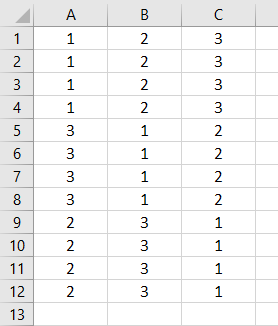
Now we need to find the area of intersection of an above data table using VBA Intersect. For this, follow the below steps:
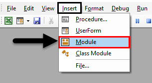
Step 1: Go to the VBA window and open a Module from the Insert menu option as shown below.
We will get a blank window of the module.
Step 2: Now write Subcategory of VBA Intersect or in any other name as per your choice.
Code:
Sub VBAIntersect1()

End Sub
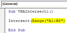
Step 3: Now directly insert Intersect command as shown below.
Code:
Sub VBAIntersect1()

Intersect(

End Sub
As we already explained the detailed syntax of Intersect, we will add an area of intersection. We can choose N number of ranges but a minimum of two Ranges should be there.
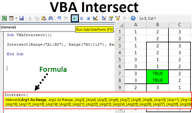
Let’s consider below an area of intersection where the first area is from A1 to B8, the second area is B3 to C12 and the third area is A7 to C10. We can consider and choose any combination of a pattern of intersections.
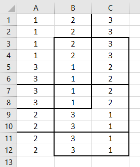
Now let’s see at what point (/s) these areas meet and intersect each other. The common area created by all the above areas will be our area of intersection.
Step 4: Now in VBA Module of Intersect, select the first area range as shown below.
Code:
Sub VBAIntersect1()

Intersect(Range("A1:B8")

End Sub
We have added the first range, but our syntax is still incomplete.
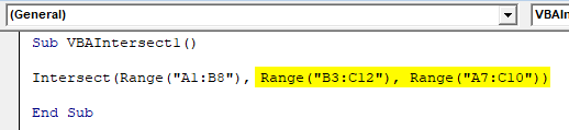
Step 5: Now further insert rest of two areas which we have discussed above separated by commas.
Code:
Sub VBAIntersect1()

Intersect(Range("A1:B8"), Range("B3:C12"), Range("A7:C10"))

End Sub
Step 6: Now give the condition as “True”.
Code:
Sub VBAIntersect1()

Intersect(Range("A1:B8"), Range("B3:C12"), Range("A7:C10")) = True

End Sub
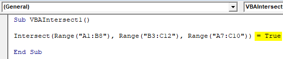
This completes our code.
Step 7: Now compile the code and run by clicking on the Play button which is located below the menu bar as shown below.
We will get the common area or intersected area which has value TRUE as shown above. Although we got the intersect area, that TRUE has replaced the data which was there in the intersected area.
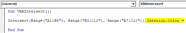
Step 8: Now to avoid losing this we can change the background of color, those common cells to any color of our choice. For this after the syntax of Intersect use Interior function along with Color as shown below.
Code:
Sub VBAIntersect1()

Intersect(Range("A1:B8"), Range("B3:C12"), Range("A7:C10")).Interior.Color =

End Sub
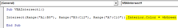
Step 9: Now in VBA, we cannot use the name of the color which we want to use directly. For this, we need to add “vb” which is used to activate the colors available in VBA. Now use it and add any name of the color of your choice. We are selecting Green here as shown below.
Code:
Sub VBAIntersect1()

Intersect(Range("A1:B8"), Range("B3:C12"), Range("A7:C10")).Interior.Color = vbGreen

End Sub
Step 10: Now again compile the written code in one go as the code is quite small and run it.
We will see the color of the intersected area is changed to Green and common area which is created by the intersection of different 3 areas in B7 to B8.
VBA Intersect – Example #2
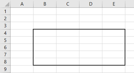
There is another but a quite a different way to use VBA Intersect. This time we use intersect in a specific worksheet. In Sheet2 we have marked an area from B4 to E8 as shown below.
Follow the below steps:
Step 1: In VBA, go to Sheet2 of current Workbook as shown below.
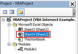
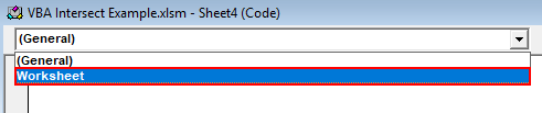
Step 2: Now select the Worksheet from this first drop down option. This will allow the code to be used in this current sheet only.
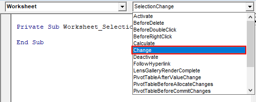
Step 3: And from the second drop-down select the option Change as shown below. This is used to target the changes done in the selected range.
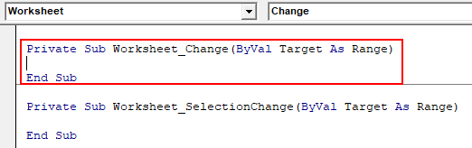
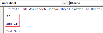
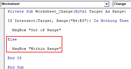
Step 4: We will write our code in the first Subcategory only.
Code:
Private Sub Worksheet_Change(ByVal Target As Range)

End Sub
Step 5: We will use the If-Else loop for forming a condition for intersect function.
Code:
Private Sub Worksheet_Change(ByVal Target As Range)

If

End If

End Sub
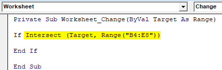
Step 6: First select the target range from B4 to E8 as shown below. This will target intersect of the area covered in B4 to E8 mainly.
Code:
Private Sub Worksheet_Change(ByVal Target As Range)

If Intersect(Target, Range("B4:E8"))

End If

End Sub
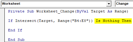
Step 7: And if there is nothing in the target area then we need to write a statement which will redirect the code ahead.
Code:
Private Sub Worksheet_Change(ByVal Target As Range)

If Intersect(Target, Range("B4:E8")) Is Nothing Then

End If

End Sub
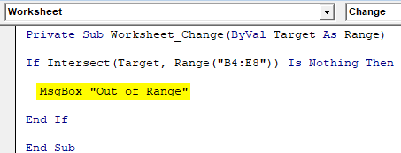
Step 8: And if really the target is out of range, we can use a message box with a message of alert as shown below.
Code:
Private Sub Worksheet_Change(ByVal Target As Range)

If Intersect(Target, Range("B4:E8")) Is Nothing Then

  MsgBox "Out of Range"

End If

End Sub
Step 9: And In the Else statement where something in written inside the box then we should get a prompt message if the written content is inside the box as shown below.
Code:
Private Sub Worksheet_Change(ByVal Target As Range)

If Intersect(Target, Range("B4:E8")) Is Nothing Then

  MsgBox "Out of Range"

Else

  MsgBox "Within Range"

End If

End Sub
Step 10: Now compile each step of written code and close the worksheet of VBA. As we have written the code specific to the sheet then it will work in the same.
Step 11: Now write something inside the box.
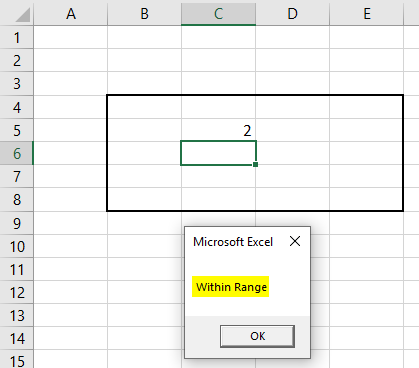
As we can see we wrote 2 in cell C5 inside the box we got the message or “Within Range”.
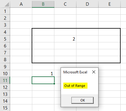
Step 12: Again write something out of the box. We wrote 1 in cell B10 and we got the message of “Out of Range” as shown below.
This is another way to using Intersect in Excel VBA.
Pros of Excel VBA Intersect
- It is very easy to at least highlight the area which intersects by the process of example-1.
- This is very useful where we need to filter or work on that kind of data which has intersection from a different area such as Dates, Owner, etc.
Things to Remember
- Remember to save the file in Macro Enable Excel format, so that code will function in every use.
- Writing code in Sheet instead of the module as shown in example-2, make the code applicable only for that sheet. That code will not work on any other sheet.
- Using Target Range as shown in example-2 is useful in specifying the area to hit.
Recommended Articles
This is a guide to VBA Intersect. Here we discuss how to use Excel VBA Intersect Function along with some practical examples and downloadable excel template. You can also go through our other suggested articles –
- VBA Loops
- VBA Web Scraping
- VBA Do Until Loop
- VBA CDEC