
-
#1
Dear all
I have put up the below code under ‘ThisWorkbook’ section and my intent is to check if a rectangle shape (its 13th) text is «YES» and if none of the cell in range «E36:E45» is colored (GREEN), then it must not allow user to move forward to next sheet..If atleast any one cell is colored, then it must not do anything(Must allow).
I dont know what mistake i am doing here…
Below code throws a message even if atleast one cell is colored.. (While it must do this if none of the cells are colored)
Code:
Private Sub Workbook_SheetDeactivate(ByVal Sh As Object)Dim Counter As Long
Dim Gcell As Range
Dim flg As Boolean
Counter = 0
If Sh.Shapes("Rectangle 13").TextFrame.Characters.Text = "YES" Then
For Each Gcell In Range("E36:E45")
        If Gcell.Interior.Color = 65280 Then Counter = Counter + 1
    Next
    If Counter = 0 Then
        Application.EnableEvents = False
        Sh.Activate
        Application.EnableEvents = True
        MsgBox "None of the cells are colored " & Sh.Name, vbExclamation, "Check of color cells"
    End If
  End If
End Sub
Please suggest.
How to create a cell-sized chart?
Tiny charts, called Sparklines, were added to Excel 2010. Look for Sparklines on the Insert tab.
-
#2
Code:
Private Sub Workbook_SheetDeactivate(ByVal Sh As Object)Dim Counter As Long
Dim Gcell As Range
Dim flg As Boolean
Counter = 0
If Sh.Shapes("Rectangle 13").TextFrame.Characters.Text = "YES" Then
For Each Gcell In Range("E36:E45")
        If Gcell.Interior.Color = 65280 Then Counter = Counter + 1 [COLOR=#ff0000][B]: Exit Sub[/B][/COLOR]
    Next
    If Counter = 0 Then
        Application.EnableEvents = False
        Sh.Activate
        Application.EnableEvents = True
        MsgBox "None of the cells are colored " & Sh.Name, vbExclamation, "Check of color cells"
    End If
  End If
End Sub
-
#3
Or maybe this:
Code:
Private Sub Workbook_SheetDeactivate(ByVal Sh As Object)Dim Counter As Long
    Dim Gcell As Range
    Dim flg As Boolean

    If Sh.Shapes("Rectangle 13").TextFrame.Characters.Text = "YES" Then
        For Each Gcell In Range("E36:E45")
            If Gcell.Interior.Color = 65280 Then Exit Sub
        Next
    End If
    Application.EnableEvents = False
    Sh.Activate
    Application.EnableEvents = True
    MsgBox "None of the cells are colored " & Sh.Name, vbExclamation, "Check of color cells"
End Sub
-
#4
Doesn’t seem to work…It still throws up the message..
-
#5
How is the cell getting its color? From the user filling the cell or from Conditional Formatting?
-
#6
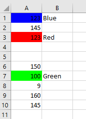
cells are colored Using below code
Code:
Private Sub Worksheet_SelectionChange(ByVal Target As Range)
Const WS_RANGE As String = "E36:E45"


On Error GoTo ws_exit
Application.EnableEvents = False
If Not Intersect(Target, Me.Range(WS_RANGE)) Is Nothing Then
  With Target
     If Selection.Interior.Color = 16777215 Then
     Selection.Interior.Color = 65280
Else
     Selection.Interior.Color = 16777215
     End If
  End With
End If


ws_exit:
Application.EnableEvents = True


End Sub
![]()
![]()
![]()
-
Solved
![]()
Содержание
- VBA Excel. Цвет ячейки (заливка, фон)
- Свойство .Interior.Color объекта Range
- Заливка ячейки цветом в VBA Excel
- Вывод сообщений о числовых значениях цветов
- Использование предопределенных констант
- Цветовая модель RGB
- Очистка ячейки (диапазона) от заливки
- Свойство .Interior.ColorIndex объекта Range
- 86 комментариев для “VBA Excel. Цвет ячейки (заливка, фон)”
- Using Conditional Formatting with Excel VBA
- Excel Conditional Formatting
- Conditional Formatting in VBA
- Practical Uses of Conditional Formatting in VBA
- A Simple Example of Creating a Conditional Format on a Range
- Multi-Conditional Formatting
- Deleting a Rule
- VBA Coding Made Easy
- Changing a Rule
- Using a Graduated Color Scheme
- Conditional Formatting for Error Values
- Conditional Formatting for Dates in the Past
- Using Data Bars in VBA Conditional Formatting
- Using Icons in VBA Conditional Formatting
- Using Conditional Formatting to Highlight Top Five
- Significance of StopIfTrue and SetFirstPriority Parameters
- Using Conditional Formatting Referencing Other Cell Values
- Operators that can be used in Conditional formatting Statements
- VBA Code Examples Add-in
VBA Excel. Цвет ячейки (заливка, фон)
Заливка ячейки цветом в VBA Excel. Фон ячейки. Свойства .Interior.Color и .Interior.ColorIndex. Цветовая модель RGB. Стандартная палитра. Очистка фона ячейки.
Свойство .Interior.Color объекта Range
Начиная с Excel 2007 основным способом заливки диапазона или отдельной ячейки цветом (зарисовки, добавления, изменения фона) является использование свойства .Interior.Color объекта Range путем присваивания ему значения цвета в виде десятичного числа от 0 до 16777215 (всего 16777216 цветов).
Заливка ячейки цветом в VBA Excel
Пример кода 1:
Поместите пример кода в свой программный модуль и нажмите кнопку на панели инструментов «Run Sub» или на клавиатуре «F5», курсор должен быть внутри выполняемой программы. На активном листе Excel ячейки и диапазон, выбранные в коде, окрасятся в соответствующие цвета.
Есть один интересный нюанс: если присвоить свойству .Interior.Color отрицательное значение от -16777215 до -1, то цвет будет соответствовать значению, равному сумме максимального значения палитры (16777215) и присвоенного отрицательного значения. Например, заливка всех трех ячеек после выполнения следующего кода будет одинакова:
Проверено в Excel 2016.
Вывод сообщений о числовых значениях цветов
Числовые значения цветов запомнить невозможно, поэтому часто возникает вопрос о том, как узнать числовое значение фона ячейки. Следующий код VBA Excel выводит сообщения о числовых значениях присвоенных ранее цветов.
Пример кода 2:
Вместо вывода сообщений можно присвоить числовые значения цветов переменным, объявив их как Long.
Использование предопределенных констант
В VBA Excel есть предопределенные константы часто используемых цветов для заливки ячеек:
| Предопределенная константа | Наименование цвета |
|---|---|
| vbBlack | Черный |
| vbBlue | Голубой |
| vbCyan | Бирюзовый |
| vbGreen | Зеленый |
| vbMagenta | Пурпурный |
| vbRed | Красный |
| vbWhite | Белый |
| vbYellow | Желтый |
| xlNone | Нет заливки |
Присваивается цвет ячейке предопределенной константой в VBA Excel точно так же, как и числовым значением:
Пример кода 3:
Цветовая модель RGB
Цветовая система RGB представляет собой комбинацию различных по интенсивности основных трех цветов: красного, зеленого и синего. Они могут принимать значения от 0 до 255. Если все значения равны 0 — это черный цвет, если все значения равны 255 — это белый цвет.
Выбрать цвет и узнать его значения RGB можно с помощью палитры Excel:
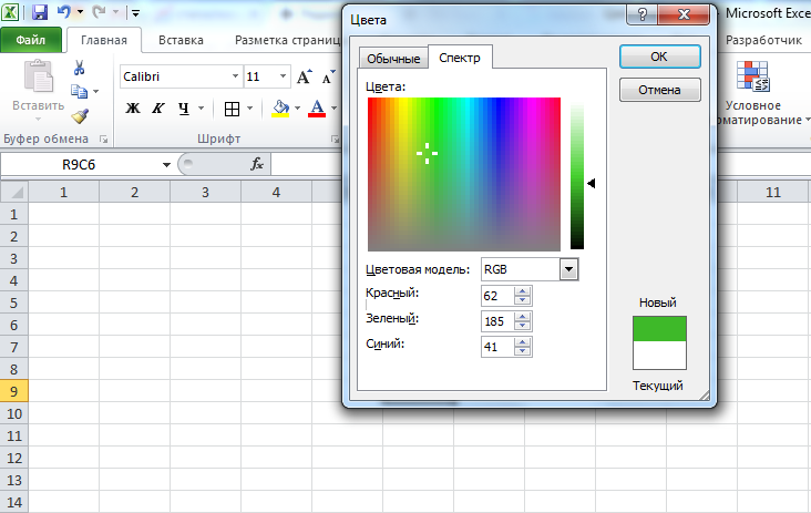
Чтобы можно было присвоить ячейке или диапазону цвет с помощью значений RGB, их необходимо перевести в десятичное число, обозначающее цвет. Для этого существует функция VBA Excel, которая так и называется — RGB.
Пример кода 4:
Список стандартных цветов с RGB-кодами смотрите в статье: HTML. Коды и названия цветов.
Очистка ячейки (диапазона) от заливки
Для очистки ячейки (диапазона) от заливки используется константа xlNone :
Свойство .Interior.ColorIndex объекта Range
До появления Excel 2007 существовала только ограниченная палитра для заливки ячеек фоном, состоявшая из 56 цветов, которая сохранилась и в настоящее время. Каждому цвету в этой палитре присвоен индекс от 1 до 56. Присвоить цвет ячейке по индексу или вывести сообщение о нем можно с помощью свойства .Interior.ColorIndex:
Пример кода 5:
Просмотреть ограниченную палитру для заливки ячеек фоном можно, запустив в VBA Excel простейший макрос:
Пример кода 6:
Номера строк активного листа от 1 до 56 будут соответствовать индексу цвета, а ячейка в первом столбце будет залита соответствующим индексу фоном.
Подробнее о стандартной палитре Excel смотрите в статье: Стандартная палитра из 56 цветов, а также о том, как добавить узор в ячейку.
86 комментариев для “VBA Excel. Цвет ячейки (заливка, фон)”
Спасибо, наконец то разобрался во всех перипетиях заливки и цвета шрифта.
Пожалуйста, Виктор. Очень рад, что статья пригодилась.
как проверить наличие фона?
Привет, Надежда!
Фон у ячейки есть всегда, по умолчанию — белый. Отсутствие цветного фона можно определить, проверив, является ли цвет ячейки белым:
Подскажите пожалуйста, как можно посчитать количество залитых определенным цветом ячеек в таблице?
Привет, Иван!
Посчитать ячейки с одинаковым фоном можно с помощью цикла.
Для реализации этого примера сначала выбираем в таблице ячейку с нужным цветом заливки. Затем запускаем код, который определяет цветовой индекс фона активной ячейки, диапазон таблицы вокруг нее и общее количество ячеек с такой заливкой в таблице.
Каким образом можно использовать не в процедуре, а именно в пользовательской функции VBA свойство .Interior.Color?
Скажем, проверять функцией значение какой-то ячейки и подкрашивать ячейку в зависимости от этого.
Фарин, пользовательская функция VBA предназначена только для возврата вычисленного значения в ячейку, в которой она расположена. Она не позволяет внутри себя менять формат своей ячейки, а также значения и форматы других ячеек.
Однако, с помощью пользовательской функции VBA можно вывести значения свойств ячейки, в которой она размещена:
В сети есть эксперименты по изменению значений других ячеек из пользовательской функции VBA, но они могут работать нестабильно и приводить к ошибкам.
Для подкрашивания ячейки в зависимости от ее значения используйте процедуру Sub или штатный инструмент Excel – условное форматирование.
а как можно закрасить только пустые ячейки ?
Лев, закрасить пустые ячейки можно с помощью цикла For Each… Next:
Евгений, спасибо за ссылку на интересный прием.
Евгений, день добрый.
Подскажите пожалуйста, как назначить ячейке цвет через значение RGB, которое в ней записано. Или цвет другой ячейки.
Привет, Александр!
Используйте функцию InStr, чтобы найти положение разделителей, а дальше функции Left и Mid. Смотрите пример с пробелом в качестве разделителя:
Или еще проще с помощью функции Split:
Добрый день!
подскажите, пожалуйста, как можно выводить из таблицы (150 столбцов х 150 строк) адрес ячеек (списком), если они имеют заливку определенного цвета.
Заранее спасибо!
Привет, Валентина!
Используйте два цикла For…Next. Определить числовой код цвета можно с помощью выделения одной из ячеек с нужным цветом.
столбец «D» имеет разноцветную заливку
надо справа от зеленой ячейки написать «Да»
Каким-то образом надо узнать числовое значение цвета, если он не стандартный — vbGreen. Например, можно выделить ячейку с нужным цветом и записать числовое значение цвета в переменную:
Евгений, спасибо за подсказку.
Все получилось
добрый день! подскажите, пожалуйста, как сделать, чтобы результаты выводились на отдельный лист ?
заранее спасибо!
Валентина, замените в коде имя «Лист2» на имя своего листа.
Евгений. Долгое время мучаюсь реализацией следующего сценария: в таблице Excel, которая является базой данных пациентов отделения есть столбец «G» в котором лаборанты отмечают исследования выполненные с контрастом «(С+)» и без «(C-)» и далее в столбце «N» они отмечаются количество использованного контраста «от 50мл до 200мл»; для удобства ввода и уменьшения числа непреднамеренных ошибок в столбцах реализована функция проверки данных что бы сотрудники могли выбирать уже готовые значения из списка и если ошибутся то выскочит ошибка; тем не менее сотрудники умудряются при заполнении таблицы не вносить количество использованного контраста. Вопрос заключается в том, как подкрасить ячейку для ввода количества контраста красным цветом при условии, что в ячейке столбца G фигурирует (С+) с целью акцентировать на этом внимание.
Заранее спасибо за ответ.
Добрый день, Алексей!
Примените условное форматирование:
1 Выберите столбец «N».
2 На вкладке ленты «Главная» перейдите по ссылкам «Условное форматирование» «Создать правило».
3 В открывшемся окне выберите тип правила: «Использовать формулу для определения форматируемых ячеек».
4 В строку формул вставьте =И(ЕСЛИ(G1=»(C+)»;1);ЕСЛИ(N1=»»;1)) . Буква «C» должна быть из одной раскладки (ENG или РУС) в формуле и в ячейке.
5 Нажмите кнопку «Формат» и на вкладке «Заливка» выберите красный цвет.
6 Закройте все окна, нажимая «OK».
Если в ячейке столбца «G» будет выбрано «(С+)», то ячейка той же строки в столбце «N» подкрасится красным цветом. После ввода значения в ячейку столбца «N», ее цвет изменится на первоначальный.
Спасибо Евгений! Ваш пример многое прояснил (в т.ч надо читать Уокенбаха и не филонить). Мне удалось заставить работать этот сценарий не так изящно как у Вас т.е создал для каждой отдельной переменной свое правило: пр. для ГМ. (С+) —> =ЕСЛИ(И(G5066=»ГМ. (С+)»;N5066=»»);»Истина»;»Ложь»)
МТ. (С+) —> =ЕСЛИ(И(G5066=»МТ. (С+)»;N5066=»»);»Истина»;»Ложь») и т.д всего 8 правил для каждого конкретного случая.
И применил их всех для столбца N:N
Ячейку G взял произвольно и в дальнейшем вообще убрал ее на лист метаданных (диапазоны переменных типа ГМ. (С+), МТ. (С+)…)
Еще раз благодарю за помощь! а есть возможность тоже самое сделать цикличным скриптом VBA ? (или я сморозил…).
Заранее спасибо за ответ.
Источник
Using Conditional Formatting with Excel VBA
In this Article
Excel Conditional Formatting
Excel Conditional Formatting allows you to define rules which determine cell formatting.
For example, you can create a rule that highlights cells that meet certain criteria. Examples include:
- Numbers that fall within a certain range (ex. Less than 0).
- The top 10 items in a list.
- Creating a “heat map”.
- “Formula-based” rules for virtually any conditional formatting.
In Excel, Conditional Formatting can be found in the Ribbon under Home > Styles (ALT > H > L).
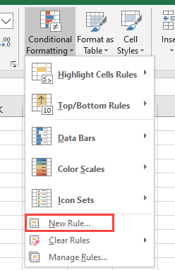
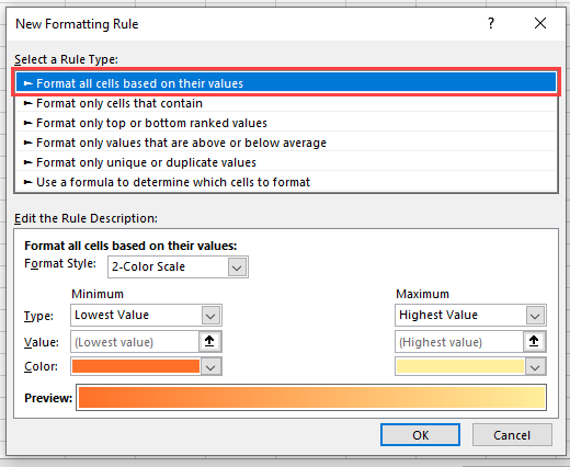
To create your own rule, click on ‘New Rule’ and a new window will appear:
Conditional Formatting in VBA
All of these Conditional Formatting features can be accessed using VBA.
Note that when you set up conditional formatting from within VBA code, your new parameters will appear in the Excel front-end conditional formatting window and will be visible to the user. The user will be able to edit or delete these unless you have locked the worksheet.
The conditional formatting rules are also saved when the worksheet is saved
Conditional formatting rules apply specifically to a particular worksheet and to a particular range of cells. If they are needed elsewhere in the workbook, then they must be set up on that worksheet as well.
Practical Uses of Conditional Formatting in VBA
You may have a large chunk of raw data imported into your worksheet from a CSV (comma-separated values) file, or from a database table or query. This may flow through into a dashboard or report, with changing numbers imported from one period to another.
Where a number changes and is outside an acceptable range, you may want to highlight this e.g. background color of the cell in red, and you can do this setting up conditional formatting. In this way, the user will be instantly drawn to this number, and can then investigate why this is happening.
You can use VBA to turn the conditional formatting on or off. You can use VBA to clear the rules on a range of cells, or turn them back on again. There may be a situation where there is a perfectly good reason for an unusual number, but when the user presents the dashboard or report to a higher level of management, they want to be able to remove the ‘alarm bells’.
Also, on the raw imported data, you may want to highlight where numbers are ridiculously large or ridiculously small. The imported data range is usually a different size for each period, so you can use VBA to evaluate the size of the new range of data and insert conditional formatting only for that range.
You may also have a situation where there is a sorted list of names with numeric values against each one e.g. employee salary, exam marks. With conditional formatting, you can use graduated colors to go from highest to lowest, which looks very impressive for presentation purposes.
However, the list of names will not always be static in size, and you can use VBA code to refresh the scale of graduated colors according to changes in the size of the range.
A Simple Example of Creating a Conditional Format on a Range
This example sets up conditional formatting for a range of cells (A1:A10) on a worksheet. If the number in the range is between 100 and 150 then the cell background color will be red, otherwise it will have no color.
Notice that first we define the range MyRange to apply conditional formatting.
Next we delete any existing conditional formatting for the range. This is a good idea to prevent the same rule from being added each time the code is ran (of course it won’t be appropriate in all circumstances).
Colors are given by numeric values. It is a good idea to use RGB (Red, Green, Blue) notation for this. You can use standard color constants for this e.g. vbRed, vbBlue, but you are limited to eight color choices.
There are over 16.7M colors available, and using RGB you can access them all. This is far easier than trying to remember which number goes with which color. Each of the three RGB color number is from 0 to 255.
Note that the ‘xlBetween’ parameter is inclusive so cell values of 100 or 150 will satisfy the condition.
Multi-Conditional Formatting
You may want to set up several conditional rules within your data range so that all the values in a range are covered by different conditions:
This example sets up the first rule as before, with the cell color of red if the cell value is between 100 and 150.
Two more rules are then added. If the cell value is less than 100, then the cell color is blue, and if it is greater than 150, then the cell color is yellow.
In this example, you need to ensure that all possibilities of numbers are covered, and that the rules do not overlap.
If blank cells are in this range, then they will show as blue, because Excel still takes them as having a value less than 100.
The way around this is to add in another condition as an expression. This needs to be added as the first condition rule within the code. It is very important where there are multiple rules, to get the order of execution right otherwise results may be unpredictable.
This uses the type of xlExpression, and then uses a standard Excel formula to determine if a cell is blank instead of a numeric value.
The FormatConditions object is part of the Range object. It acts in the same way as a collection with the index starting at 1. You can iterate through this object using a For…Next or For…Each loop.
Deleting a Rule
Sometimes, you may need to delete an individual rule in a set of multiple rules if it does not suit the data requirements.
This code creates a new rule for range A1:A10, and then deletes it. You must use the correct index number for the deletion, so check on ‘Manage Rules’ on the Excel front-end (this will show the rules in order of execution) to ensure that you get the correct index number. Note that there is no undo facility in Excel if you delete a conditional formatting rule in VBA, unlike if you do it through the Excel front-end.
VBA Coding Made Easy
Stop searching for VBA code online. Learn more about AutoMacro — A VBA Code Builder that allows beginners to code procedures from scratch with minimal coding knowledge and with many time-saving features for all users!

Changing a Rule
Because the rules are a collection of objects based on a specified range, you can easily make changes to particular rules using VBA. The actual properties once the rule has been added are read-only, but you can use the Modify method to change them. Properties such as colors are read / write.
This code creates a range object (A1:A10) and adds a rule for numbers between 100 and 150. If the condition is true then the cell color changes to red.
The code then changes the rule to numbers less than 10. If the condition is true then the cell color now changes to green.
Using a Graduated Color Scheme
Excel conditional formatting has a means of using graduated colors on a range of numbers running in ascending or descending order.
This is very useful where you have data like sales figures by geographical area, city temperatures, or distances between cities. Using VBA, you have the added advantage of being able to choose your own graduated color scheme, rather than the standard ones offered on the Excel front-end.
When this code is run, it will graduate the cell colors according to the ascending values in the range A1:A10.
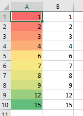
This is a very impressive way of displaying the data and will certainly catch the users’ attention.
Conditional Formatting for Error Values
When you have a huge amount of data, you may easily miss an error value in your various worksheets. If this is presented to a user without being resolved, it could lead to big problems and the user losing confidence in the numbers. This uses a rule type of xlExpression and an Excel function of IsError to evaluate the cell.
You can create code so that all cells with errors in have a cell color of red:
Conditional Formatting for Dates in the Past
You may have data imported where you want to highlight dates that are in the past. An example of this could be a debtors’ report where you want any old invoice dates over 30 days old to stand out.
This code uses the rule type of xlExpression and an Excel function to evaluate the dates.
This code will take a range of dates in the range A1:A10, and will set the cell color to red for any date that is over 30 days in the past.
In the formula being used in the condition, Now() gives the current date and time. This will keep recalculating every time the worksheet is recalculated, so the formatting will change from one day to the next.
Using Data Bars in VBA Conditional Formatting
You can use VBA to add data bars to a range of numbers. These are almost like mini charts, and give an instant view of how large the numbers are in relation to each other. By accepting default values for the data bars, the code is very easy to write.
Your data will look like this on the worksheet:
Using Icons in VBA Conditional Formatting
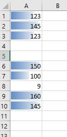
You can use conditional formatting to put icons alongside your numbers in a worksheet. The icons can be arrows or circles or various other shapes. In this example, the code adds arrow icons to the numbers based on their percentage values:
This will give an instant view showing whether a number is high or low. After running this code, your worksheet will look like this:
Using Conditional Formatting to Highlight Top Five
You can use VBA code to highlight the top 5 numbers within a data range. You use a parameter called ‘AddTop10’, but you can adjust the rank number within the code to 5. A user may wish to see the highest numbers in a range without having to sort the data first.
The data on your worksheet would look like this after running the code:
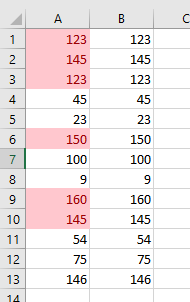
Note that the value of 145 appears twice so six cells are highlighted.
Significance of StopIfTrue and SetFirstPriority Parameters
StopIfTrue is of importance if a range of cells has multiple conditional formatting rules to it. A single cell within the range may satisfy the first rule, but it may also satisfy subsequent rules. As the developer, you may want it to display the formatting only for the first rule that it comes to. Other rule criteria may overlap and may make unintended changes if allowed to continue down the list of rules.
The default on this parameter is True but you can change it if you want all the other rules for that cell to be considered:
The SetFirstPriority parameter dictates whether that condition rule will be evaluated first when there are multiple rules for that cell.
This moves the position of that rule to position 1 within the collection of format conditions, and any other rules will be moved downwards with changed index numbers. Beware if you are making any changes to rules in code using the index numbers. You need to make sure that you are changing or deleting the right rule.
You can change the priority of a rule:
This will change the relative positions of any other rules within the conditional format list.
Using Conditional Formatting Referencing Other Cell Values
This is one thing that Excel conditional formatting cannot do. However, you can build your own VBA code to do this.
Suppose that you have a column of data, and in the adjacent cell to each number, there is some text that indicates what formatting should take place on each number.
The following code will run down your list of numbers, look in the adjacent cell for formatting text, and then format the number as required:
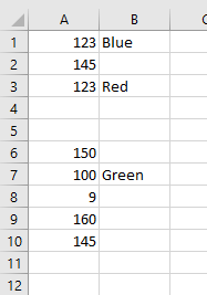
Once this code has been run, your worksheet will now look like this:
The cells being referred to for the formatting could be anywhere on the worksheet, or even on another worksheet within the workbook. You could use any form of text to make a condition for the formatting, and you are only limited by your imagination in the uses that you could put this code to.
Operators that can be used in Conditional formatting Statements
As you have seen in the previous examples, operators are used to determine how the condition values will be evaluated e.g. xlBetween.
There are a number of these operators that can be used, depending on how you wish to specify your rule criteria.
| Name | Value | Description |
| xlBetween | 1 | Between. Can be used only if two formulas are provided. |
| xlEqual | 3 | Equal. |
| xlGreater | 5 | Greater than. |
| xlGreaterEqual | 7 | Greater than or equal to. |
| xlLess | 6 | Less than. |
| xlLessEqual | 8 | Less than or equal to. |
| xlNotBetween | 2 | Not between. Can be used only if two formulas are provided. |
| xlNotEqual | 4 | Not equal. |

VBA Code Examples Add-in
Easily access all of the code examples found on our site.
Simply navigate to the menu, click, and the code will be inserted directly into your module. .xlam add-in.
Источник
- Remove From My Forums
-
Question
-
Hello,
I’m trying to create an IF THEN statement in Excel VBA that will send out an email if certain cells are red. I’ve tried a few things, but nothing seems to be working. I just keep getting a 438 error whenever I run the function.
So I just want it to determine if any cells in column E are red, and if they are, proceed to the rest of the function that sends out the email. Ideally I would also like to be able to take the values of the same row in columns F and G (first name
and last name) and use that as the address (firstname.lastname@email.com), but I can work on that once I get past this first stage…Any ideas? If you need more info, just let me know!
Answers
-
Hi Josh,
I think you can traverse these cells and judge whether they are red via:
if Selection.Interior.Color = 255 then
‘ here you can call the send email funtion in your code
‘ call SendEmail
end if
or
if Selection.Interior.ColorIndex = 3 then
..
end if
I hope this can help you and just feel free to follow up after you have tried.
Best Regards,
Bruce Song [MSFT]
MSDN Community Support | Feedback to us
Get or Request Code Sample from Microsoft
Please remember to mark the replies as answers if they help and unmark them if they provide no help.
-
Marked as answer by
Tuesday, April 12, 2011 8:53 AM
-
Marked as answer by

June 29, 2015/
Chris Newman
Wishful Thinking?
Have you ever had a time where you wished you could write an IF formula in Excel based on whether or not a cell was filled with the color green or not? Unfortunately, Excel doesn’t have a built-in «IsGreen» function you can call to perform such logic. However, with the power of VBA you can write your own functions and actually call them from the Formula Bar! This can be extremely powerful and extends Excel’s logical prowess to a near limitless level! Let’s take a look at how we can add our own functions into our spreadsheets.
Where Do I Write The Function Logic?
I recommend storing your custom functions inside a VBA module. Here are the steps to create a brand new module within your spreadsheet.
-
Inside your spreadsheet use the keyboard shortcut Alt + F11 to open up the Visual Basic Editor window
-
On the left-hand side of the window, you should see a Project pane that will display every Excel workbook/add-in you currently have open
-
Find the Project Name that matches the Excel file you want to store the functions in and right-click on the Project Name
-
Inside the menu that pops up, go to Insert -> Module
-
A blank white canvas should appear on your screen and this is where you will want to write or paste in your custom function code

Examples of Functions You Can Add
This is where you can let your imagination run wild (especially if you have a good grasp on how to write VBA). But in case you are new to VBA (you can learn how to get started learning to write VBA here), I am going to provide you with a few common functions that might be useful when trying to logically analyze a cell’s formatting.
Function To Determine If Cell Text Is Bold
Function ISBOLD(cell As Range) As Boolean
‘PURPOSE: Determine if cell has bold text or not
‘SOURCE: www.TheSpreadsheetGuru.com
‘Ensure function will recalculate after spreadsheet changes
Application.Volatile True
‘Test Cell Value
On Error GoTo PartiallyBold
ISBOLD = cell.Font.Bold
On Error GoTo 0
Exit Function
‘Handle if only part of the cell value is bolded
PartiallyBold:
If Err.Number = 94 Then ISBOLD = True
End Function
Function To Determine If Cell Text Is Italicized
Function ISITALIC(cell As Range) As Boolean
‘PURPOSE: Determine if cell has italicized text or not
‘SOURCE: www.TheSpreadsheetGuru.com
‘Ensure function will recalculate after spreadsheet changes
Application.Volatile True
‘Test Cell Value
On Error GoTo PartiallyItalic
ISITALIC = cell.Font.Italic
On Error GoTo 0
Exit Function
‘Handle if only part of the cell value is italicized
PartiallyItalic:
If Err.Number = 94 Then ISITALIC = True
End Function
Function To Determine If Cell Text Is Underlined
Function ISUNDERLINED(cell As Range) As Boolean
‘PURPOSE: Determine if cell has underlined text or not
‘SOURCE: www.TheSpreadsheetGuru.com
‘Ensure function will recalculate after spreadsheet changes
Application.Volatile True
‘Test Cell Value
If cell.Font.Underline = xlNone Then
ISUNDERLINED = False
Else
ISUNDERLINED = True
End If
End Function
Function To Determine If Cell Text Is A Specific Color
Function ISFONTCOLOR(cell As Range, TargetColor As Range) As Boolean
‘PURPOSE: Test if cell font color matches a specified cell fill color
‘NOTE: Color changes will not trigger your spreadsheet to re-calculate
‘SOURCE: www.TheSpreadsheetGuru.com
‘Ensure function will recalculate after spreadsheet changes
Application.Volatile True
‘Test Cell Font Color
If cell.Font.Color = TargetColor.Interior.Color Then
ISFONTCOLOR = True
Else
ISFONTCOLOR = False
End If
End Function
Function To Determine If Cell Fill Is A Specific Color
Function ISFILLCOLOR(cell As Range, TargetColor As Range) As Boolean
‘PURPOSE: Test if cell fill color matches a specified cell fill color
‘NOTE: Color changes will not trigger your spreadsheet to re-calculate
‘SOURCE: www.TheSpreadsheetGuru.com
‘Ensure function will recalculate after spreadsheet changes
Application.Volatile True
‘Test Cell Fill Color
If cell.Interior.Color = TargetColor.Interior.Color Then
ISFILLCOLOR = True
Else
ISFILLCOLOR = False
End If
End Function
Calling A Custom Function
Once you have written your function in the VBA module, you can then start to use it! Simply begin typing the function inside the formula bar and you will see your custom function appear as a viable selection. Note that you will not get any ScreenTips with your custom functions (come on Microsoft!), so you will need to memorize how to properly use your custom function.
Formula Recalculation
You will need to be careful with these formulas since changing the format of a cell does not trigger a spreadsheet recalculation. Always make sure you hit the F9 key before you begin your analysis while using a custom function that takes into account formatting in your spreadsheets.
Download An Example File With These Functions
To help you further, I have created an example workbook with all the custom functions described in this article put to use so you can see them in action.
If you would like to get a copy of the Excel file I used throughout this article, feel free to directly download the spreadsheet by clicking the download button below.
About The Author
Hey there! I’m Chris and I run TheSpreadsheetGuru website in my spare time. By day, I’m actually a finance professional who relies on Microsoft Excel quite heavily in the corporate world. I love taking the things I learn in the “real world” and sharing them with everyone here on this site so that you too can become a spreadsheet guru at your company.
Through my years in the corporate world, I’ve been able to pick up on opportunities to make working with Excel better and have built a variety of Excel add-ins, from inserting tickmark symbols to automating copy/pasting from Excel to PowerPoint. If you’d like to keep up to date with the latest Excel news and directly get emailed the most meaningful Excel tips I’ve learned over the years, you can sign up for my free newsletters. I hope I was able to provide you with some value today and I hope to see you back here soon!
— Chris
Founder, TheSpreadsheetGuru.com
Заливка ячейки цветом в VBA Excel. Фон ячейки. Свойства .Interior.Color и .Interior.ColorIndex. Цветовая модель RGB. Стандартная палитра. Очистка фона ячейки.
Свойство .Interior.Color объекта Range
Начиная с Excel 2007 основным способом заливки диапазона или отдельной ячейки цветом (зарисовки, добавления, изменения фона) является использование свойства .Interior.Color объекта Range путем присваивания ему значения цвета в виде десятичного числа от 0 до 16777215 (всего 16777216 цветов).
Заливка ячейки цветом в VBA Excel
Пример кода 1:
|
Sub ColorTest1() Range(«A1»).Interior.Color = 31569 Range(«A4:D8»).Interior.Color = 4569325 Range(«C12:D17»).Cells(4).Interior.Color = 568569 Cells(3, 6).Interior.Color = 12659 End Sub |
Поместите пример кода в свой программный модуль и нажмите кнопку на панели инструментов «Run Sub» или на клавиатуре «F5», курсор должен быть внутри выполняемой программы. На активном листе Excel ячейки и диапазон, выбранные в коде, окрасятся в соответствующие цвета.
Есть один интересный нюанс: если присвоить свойству .Interior.Color отрицательное значение от -16777215 до -1, то цвет будет соответствовать значению, равному сумме максимального значения палитры (16777215) и присвоенного отрицательного значения. Например, заливка всех трех ячеек после выполнения следующего кода будет одинакова:
|
Sub ColorTest11() Cells(1, 1).Interior.Color = —12207890 Cells(2, 1).Interior.Color = 16777215 + (—12207890) Cells(3, 1).Interior.Color = 4569325 End Sub |
Проверено в Excel 2016.
Вывод сообщений о числовых значениях цветов
Числовые значения цветов запомнить невозможно, поэтому часто возникает вопрос о том, как узнать числовое значение фона ячейки. Следующий код VBA Excel выводит сообщения о числовых значениях присвоенных ранее цветов.
Пример кода 2:
|
Sub ColorTest2() MsgBox Range(«A1»).Interior.Color MsgBox Range(«A4:D8»).Interior.Color MsgBox Range(«C12:D17»).Cells(4).Interior.Color MsgBox Cells(3, 6).Interior.Color End Sub |
Вместо вывода сообщений можно присвоить числовые значения цветов переменным, объявив их как Long.
Использование предопределенных констант
В VBA Excel есть предопределенные константы часто используемых цветов для заливки ячеек:
| Предопределенная константа | Наименование цвета |
|---|---|
| vbBlack | Черный |
| vbBlue | Голубой |
| vbCyan | Бирюзовый |
| vbGreen | Зеленый |
| vbMagenta | Пурпурный |
| vbRed | Красный |
| vbWhite | Белый |
| vbYellow | Желтый |
| xlNone | Нет заливки |
Присваивается цвет ячейке предопределенной константой в VBA Excel точно так же, как и числовым значением:
Пример кода 3:
|
Range(«A1»).Interior.Color = vbGreen |
Цветовая модель RGB
Цветовая система RGB представляет собой комбинацию различных по интенсивности основных трех цветов: красного, зеленого и синего. Они могут принимать значения от 0 до 255. Если все значения равны 0 — это черный цвет, если все значения равны 255 — это белый цвет.
Выбрать цвет и узнать его значения RGB можно с помощью палитры Excel:
Палитра Excel
Чтобы можно было присвоить ячейке или диапазону цвет с помощью значений RGB, их необходимо перевести в десятичное число, обозначающее цвет. Для этого существует функция VBA Excel, которая так и называется — RGB.
Пример кода 4:
|
Range(«A1»).Interior.Color = RGB(100, 150, 200) |
Список стандартных цветов с RGB-кодами смотрите в статье: HTML. Коды и названия цветов.
Очистка ячейки (диапазона) от заливки
Для очистки ячейки (диапазона) от заливки используется константа xlNone:
|
Range(«A1»).Interior.Color = xlNone |
Свойство .Interior.ColorIndex объекта Range
До появления Excel 2007 существовала только ограниченная палитра для заливки ячеек фоном, состоявшая из 56 цветов, которая сохранилась и в настоящее время. Каждому цвету в этой палитре присвоен индекс от 1 до 56. Присвоить цвет ячейке по индексу или вывести сообщение о нем можно с помощью свойства .Interior.ColorIndex:
Пример кода 5:
|
Range(«A1»).Interior.ColorIndex = 8 MsgBox Range(«A1»).Interior.ColorIndex |
Просмотреть ограниченную палитру для заливки ячеек фоном можно, запустив в VBA Excel простейший макрос:
Пример кода 6:
|
Sub ColorIndex() Dim i As Byte For i = 1 To 56 Cells(i, 1).Interior.ColorIndex = i Next End Sub |
Номера строк активного листа от 1 до 56 будут соответствовать индексу цвета, а ячейка в первом столбце будет залита соответствующим индексу фоном.
Подробнее о стандартной палитре Excel смотрите в статье: Стандартная палитра из 56 цветов, а также о том, как добавить узор в ячейку.
The IF…THEN statement is one of the most commonly used and most useful statements in VBA. The IF…THEN statement allows you to build logical thinking inside your macro.
The IF…THEN statement is like the IF function in Excel. You give the IF a condition to test, such as “Is the customer a “preferred” customer?” If the customer is classified as “preferred” then calculate a discount amount. Another test could be to test the value of a cell, such as “Is the cell value greater than 100?” If so, display the message “Great sale!” Otherwise, display the message “Better luck next time.”
The IF…THEN can also evaluate many conditions. Like the AND function, you can ask several questions and all the questions must evaluate to TRUE to perform the action. Similarly, you can ask several questions and if any single or multiple of questions are true, the action will be performed. This is like an OR function in Excel.
Task #1 – Simple IF
In this example we will evaluate a single cell. Once we have the logic correct, we will apply the logic to a range of cells using a looping structure.
In Excel, open the VBA Editor by pressing F-11 (or press the Visual Basic button on the Developer ribbon.)
Right-click “This Workbook” in the Project Explorer (upper-left of VBA Editor) and select Insert ⇒ Module.

In the Code window (right panel) type the following and press ENTER.
Sub Simple_If()
We want to evaluate the contents of cell B9 to determine if the value is greater than 0 (zero). If the value is >0, we will display the value of cell B9 in cell C9.
In the Code window, click between the Sub and End Sub commands and enter the following.
If Range("B9").Value > 0 Then Range("C9").Value = Range("B9").Value
If you only have a single action to perform, you can leave all the code on a single line and you do not have to close the statement with an END IF.
If you have more than one action to perform, you will want to break your code into multiple lines like the following example.

When using this line-break style, don’t forget to include the END IF statement at the end of the logic.
Test the function by executing the macro. Click in the code and press F5 or click the Run ![]() button on the toolbar at the top of the VBA Editor window.
button on the toolbar at the top of the VBA Editor window.
The number 45 should appear in cell C9.

If we change the value in cell B9 to -2, clear the contents of cell C9 and re-run the macro, cell C9 will remain blank.

Suppose we want to test the values in Column B to see if they are between 1 and 400. We will use an AND statement to allow the IF to perform multiple tests.
Update the code with the following IF statement.
Sub Simple_If()
	If Range("B9").Value > 0 And Range("B9").Value <= 400 Then
		Range("C9").Value = Range("B9").Value
	End If
End Sub
Test the macro by changing the value in cell B9 to values between 1 and 400 as well as testing values >400 or <=0 (remember to clear the contents of cell C9 prior to each test).
Task #2 – Color all values between 1 and 400 green (Looping Through Data)
Now we want to loop through the values in Column B and perform the test on each value.
Below the existing procedure, start a new procedure named IF_Loop(). Type the following and press ENTER.
Sub IF_Loop()
We want to color all the cells in range B9:B18 green if their cell value is between 1 and 400.
There are many ways to determine the data’s range. For examples of several range detection/selection techniques, click the link below to check out the VBA & Macros course.
Unlock Excel VBA and Excel Macros
The technique we will use is to convert the plain table to a Data Table and use Table References. Table References are great because they automatically expand and contract when data is either added or removed from the table. This keep you from having to update all your formulas and VBA code when data ranges change, which they often do.
Click anywhere in the table and press CTRL-T and then click OK.
We want to restore our original cell colors. Select Table Tools ⇒ Design ⇒ Table Styles (group) ⇒ Expand the table styles list and select Clear (bottom of list).

Rename the table (upper-left) to “TableSales”.

Select cell D7 (or any blank cell) and type an equal’s sign.
=Select cells B9:B18 and note the update to the formula. This contains the proper method for referring to table fields (columns).
=TableSales[Sales]
Highlight the reference in the formula bar (do not include the equal’s sign) and press CTRL-C to copy the reference into memory.

Press ESC to abandon the formula.
Return to the VBA Editor and click between the Sub and End Sub commands in the IF_Loop() procedure.
We want to loop through the sales column of the table. For detailed information on creating and managing looping structures, click the link below.
Excel VBA: Loop through cells inside the used range (For Each Collection Loop)
We want the cell color to change to green if the cell’s value is between 1 and 400. We can use the Interior object to set the Color property to green. Enter the following code in the VBA Editor.
Sub IF_Loop()
	Dim cell As Range
	For Each cell In Range("TableSales[Sales]")
		If cell.Value > 0 And cell.Value <= 400 Then
			cell.Interior.Color = VBA.ColorConstants.vbGreen
		End If
	Next cell
End Sub
Run the updated code to see the results as witnessed below.

The color green is a bit on the bright side. We want a pale green, but we don’t know the color code for pale green. Here is a great way to discover the color of any cell.
Open the Immediate Windows by pressing CTRL-G or clicking View à Immediate Window from the VBA Editor toolbar. This should present the Immediate Window in the lower portion of the VBA Editor.
Select an empty cell and set the fill color to a pale green.

With the newly colored cell selected, click in the Immediate Window of the VBA Editor and enter the following text and press ENTER.
? activecell.Interior.Color
The above command will return the value of the active cell’s fill color. In this case, pale green is 9359529.
Update the VBA code to use the color code for pale green instead of the VBA green.
cell.Interior.Color = 9359529
Run the updated code and notice the colors are a more pleasant pale green.

Task #3 – Color all cells that are <=0 and >400 yellow
Now that we have identified all the numbers between 1 and 400, let’s color the remaining cells yellow. The color code for the yellow we will be using is 6740479.
To add the second possible action will require the addition of an ELSE statement at the end of our existing IF statement. Update the code with the following modification.
  Else
    cell.Interior.Color = 6740479
Run the updated code and notice how all the previously white cells are now yellow.

Task #4 – Negative values will be colored red
We will now update the code to color all the negative valued cells red. The color code for the red we will be using is 192.
To add the third possible action will require the addition of an ELSEIF statement directly after the initial IF statement. Update the code with the following modification.
 ElseIf cell.Value < 0 Then
     cell.Interior.Color = 192
Run the updated macro and observe that all the negative valued cells are now filled with the color red.

Feel free to Download the Workbook HERE.

Published on: August 23, 2018
Last modified: February 21, 2023


Leila Gharani
I’m a 5x Microsoft MVP with over 15 years of experience implementing and professionals on Management Information Systems of different sizes and nature.
My background is Masters in Economics, Economist, Consultant, Oracle HFM Accounting Systems Expert, SAP BW Project Manager. My passion is teaching, experimenting and sharing. I am also addicted to learning and enjoy taking online courses on a variety of topics.
-
03-18-2010, 01:42 PM
#1
Registered User
=IF (cell color) then?
Two part question:
1. How do I structure an IF statement based on a specific cell color (e.g. if a cell is yellow, then perform function x)
2. How do I know what color is what? Is there a pantone reference? A color «name» that excel uses?
Thanks
-
03-18-2010, 06:25 PM
#2
Re: =IF (cell color) then?
why is the cell coloured?
you can use conditional format to colour the cell then use the same criteria in a function
-
03-19-2010, 12:48 PM
#3
Registered User
Re: =IF (cell color) then?
The cells are not conditionally formatted…it is a manual process based on non-conditional input.
-
03-19-2010, 05:25 PM
#4
Re: =IF (cell color) then?
Excel does not have a built in function to determine cell color. You would need to use VBA code to determine cell color.
If you can use a VBA solution, search the Forum using terms like: Count cells by color, or Sum cells by color, etc.
To martin’s point, what logic are you using to determine cell color? If the fill color selection is a random process (no logic or consistency), then it will be a bit difficult to determine which cells to reference in any formula.
Sum/Count Cells By Fill Or Background Color in Excel
Palmetto
Do you know . . . ?
You can leave feedback and add to the reputation of all who contributed a helpful response to your solution by clicking the star icon located at the left in one of their post in this thread.
-
03-19-2010, 05:28 PM
#5
Re: =IF (cell color) then?
-
06-17-2011, 08:56 AM
#6
Registered User
Re: =IF (cell color) then?
I could use help with this also, to be specific, I am taking data and assigning it a confidence level. The confidence level is going to be indicated by the use of cell background color, ie a green cell indicates a +/- 10% confidence level and therefore my expected data rande is X+(X*.1) and X-(X*.1) and so on (X being my measured sampled.
How do I create function so that IF the cell is one it uses one confidence level, if its another then a different one, etc?
-
08-25-2013, 02:00 PM
#7
Registered User
Re: =IF (cell color) then?
I know I am digging an old post here, but I wonder if the new excel 2013, has a solution to this. I am manually colouring a cell and want it show an x value (referenced from a different cell), if the colour is say green and a 0 if its red.
-
08-25-2013, 02:12 PM
#8
Re: =IF (cell color) then?
on_way_to_fame,
Unfortunately you need to post your question in a new thread, it’s against the forum rules to post a question in the thread of another user. If you create your own thread, any advice will be tailored to your situation so you should include a description of what you’ve done and are trying to do. Also, if you feel that this thread is particularly relevant to what you are trying to do, you can surely include a link to it in your new thread.
If I have helped, Don’t forget to add to my reputation (click on the star below the post)
Don’t forget to mark threads as «Solved» (Thread Tools->Mark thread as Solved)
Use code tags when posting your VBA code: [code] Your code here [/code]
-
08-25-2013, 10:37 PM
#9
Registered User
Re: =IF (cell color) then?
Hi,
Apologies for that. I will create a new thread for this.
-
04-25-2014, 10:10 AM
#10
Re: =IF (cell color) then?
Writing a macro that creates a function (customized excel formula) is the trick you are looking for. What is the «perform x» that you want it to do exactly?
-
11-05-2014, 12:37 PM
#11
Registered User
Re: =IF (cell color) then?
On_way_to_fame,
Did you ever find a solution to your problem? I am trying to do the same thing.
-
11-05-2014, 12:42 PM
#12
Re: =IF (cell color) then?
baffled, perhaps you missed reading post #8?
1. Use code tags for VBA. [code] Your Code [/code] (or use the # button)
2. If your question is resolved, mark it SOLVED using the thread tools
3. Click on the star if you think someone helped youRegards
Ford


