
VBA that checks if a cell is in a range, named range, or any kind of range, in Excel.
Sections:
Check if Cell is in a Range Macro
Check if Cell is in a Named Range
Notes
Check if Cell is in a Range Macro
Sub CellinRange()
'######################################'
'######### TeachExcel.com #########'
'######################################'
'Tests if a Cell is within a specific range.
Dim testRange As Range
Dim myRange As Range
'Set the range
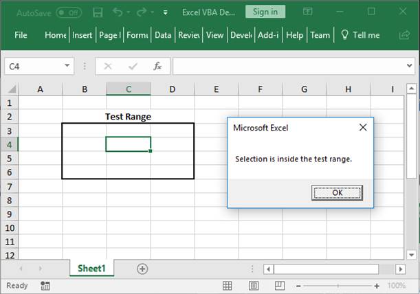
Set testRange = Range("B3:D6")
'Get the cell or range that the user selected
Set myRange = Selection
'Check if the selection is inside the range.
If Intersect(testRange, myRange) Is Nothing Then
'Selection is NOT inside the range.
MsgBox "Selection is outside the test range."
Else
'Selection IS inside the range.
MsgBox "Selection is inside the test range."
End If
End Sub
How to Use the Macro
B3:D6 change this to the range that you want to check to see if the cell is within it.
Selection keep this the same to use the currently selected cell or range from the user or change it to a regular hard-coded range reference like Range(«A1») or whatever range you want.
‘Selection is NOT inside the range. under this line, put the code that you want to run when the cell is not within the range.
‘Selection IS inside the range. under this line, put the code that you want to run when the cell is within the range.
How Does the Macro Know if the Cell is in the Range?
Intersect(testRange, myRange) this checks if the range within the myRange variable overlaps or intersects with the range in the testRange variable. This function, the Intersect function, will return a range object where the two ranges overlap, or, if they don’t overlap, it will return nothing.
As such, we can use the IF statement to check if nothing was returned or not and we do that using Is Nothing after the Intersect function. The Is Nothing is what checks if the Intersect function returned nothing or not, which evaluates to TRUE or FALSE, which is then used by the IF statement to complete its logic and run.
This is how we get the full first line of the IF statement, and this is where all the magic happens:
If Intersect(testRange, myRange) Is Nothing Then
The rest of the IF statement is just a regular IF statement in VBA, with a section of code that runs if the cell is within the range and one that runs when the cell is outside of the range.
Check if Cell is in a Named Range
This is almost exactly the same as the previous macro except that we need to change the range reference from B3:D6 to the name of the named range; that’s it.
It could look like this:
Sub CellinRange()

'######################################'
'#########   TeachExcel.com   #########'
'######################################'

'Tests if a Cell is within a specific range.

Dim testRange As Range
Dim myRange As Range

'Set the range
Set testRange = Range("MyNamedRange")

'Get the cell or range that the user selected
Set myRange = Selection

'Check if the selection is inside the range.
If Intersect(testRange, myRange) Is Nothing Then
    'Selection is NOT inside the range.

    MsgBox "Selection is outside the test range."

Else
    'Selection IS inside the range.

    MsgBox "Selection is inside the test range."

End If

End Sub
For a more detailed expanation of how this macro works, look to the section above.
Notes
If the user makes a selection of multiple cells or a range, and any of those cells are within the test range, this macro will run the code for when the selection is inside the range.
Testing if a range is within a range simply uses the Intersect function in Excel VBA; however, due to how it works, it can seem confusing since we have to check if it Is Nothing or not. But, once you get used to writing this and seeing this in IF statements, it’s really not that difficult, just remember that, in this instance, you will want to pair the use of Intersect with Is Nothing and everything else should follow quite easily.
Download the sample file to get the macro in Excel.
Similar Content on TeachExcel
Excel Data Validation — Limit What a User Can Enter into a Cell
Tutorial:
Data Validation is a tool in Excel that you can use to limit what a user can enter into a…
Logical Operators in Excel VBA Macros
Tutorial: Logical operators in VBA allow you to make decisions when certain conditions are met.
They…
Make a UserForm in Excel
Tutorial: Let’s create a working UserForm in Excel.
This is a step-by-step tutorial that shows you e…
Sum Values that Equal 1 of Many Conditions across Multiple Columns in Excel
Tutorial:
How to Sum values using an OR condition across multiple columns, including using OR with …
VBA Comparison Operators
Tutorial: VBA comparison operators are used to compare values in VBA and Macros for Excel.
List of V…
Subscribe for Weekly Tutorials
BONUS: subscribe now to download our Top Tutorials Ebook!
EXPLANATION
This tutorial shows how to test if a range contains a specific value and return a specified value if the formula tests true or false, by using an Excel formula and VBA.
This tutorial provides one Excel method that can be applied to test if a range contains a specific value and return a specified value by using an Excel IF and COUNTIF functions. In this example, if the Excel COUNTIF function returns a value greater than 0, meaning the range has cells with a value of 500, the test is TRUE and the formula will return a «In Range» value. Alternatively, if the Excel COUNTIF function returns a value of of 0, meaning the range does not have cells with a value of 500, the test is FALSE and the formula will return a «Not in Range» value.
This tutorial provides one VBA method that can be applied to test if a range contains a specific value and return a specified value.
FORMULA
=IF(COUNTIF(range, value)>0, value_if_true, value_if_false)
ARGUMENTS
range: The range of cells you want to count from.
value: The value that is used to determine which of the cells should be counted, from a specified range, if the cells’ value is equal to this value.
value_if_true: Value to be returned if the range contains the specific value
value_if_false: Value to be returned if the range does not contains the specific value.
In Microsoft Excel, we can determine if a Cell is within a Range with IF Function, however, when it comes to identify the same via VBA code then we need to use if statement. Below is the VBA code and process which you need to paste in the code module of your file.
1. Open Excel
2. Press ALT + F11
3. The VBA Editor will open.
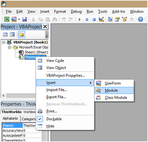
4. Click anywhere in the Project Window.
5. Click on Insert
6. Click on Module
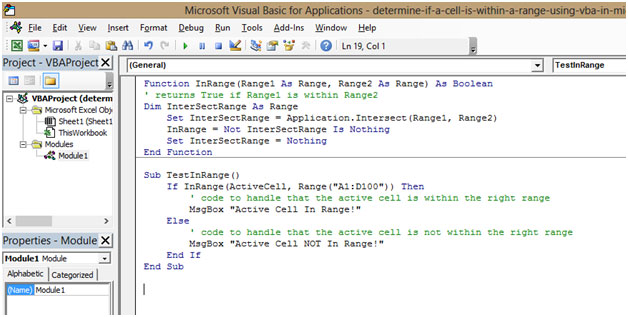
7. In the Code Window, Copy and Paste the below mentioned Code
Function InRange(Range1 As Range, Range2 As Range) As Boolean
‘ returns True if Range1 is within Range2
Dim InterSectRange As Range
Set InterSectRange = Application.InterSect(Range1, Range2)
InRange = Not InterSectRange Is Nothing
Set InterSectRange = Nothing
End FunctionSub TestInRange()
If InRange(ActiveCell, Range(«A1:D100»)) Then
‘ code to handle that the active cell is within the right range
MsgBox «Active Cell In Range!»»»
Else
‘ code to handle that the active cell is not within the right range
MsgBox «Active Cell NOT In Range!»»»
End If
End Sub
8. Once this is pasted, go to the Excel file
9. Select cell A1
10. Click on the VIEW Tab on the ribbon
11. Click on Macros
12. Click on View Macros
13. Shortcut Key to View Macros is ALT + F8
14. A Window will popup

15. Select the Macro
16. Here the Macro is named as “TestInRange”
17. Select the Macro “TestInRange”
18. Click on Run
19. As this cell is in Range you will get a Popup which says “Active Cell In Range!”
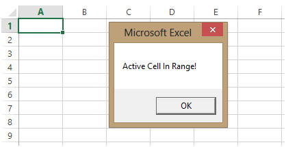
20. Click OK to close the Box
Now we will select Cell G9 which is not in Range
1. Select cell G9
2. Click on the VIEW Tab on the ribbon
3. Click on Macros
4. Click on View Macros
5. Shortcut Key to View Macros is ALT + F8
6. A Window will popup
7. Select the Macro
8. Here the Macro is named as “TestInRange”
9. Select Macro “TestInRange”
10. Click on Run
11. As this cell is not in Range you will get a Popup which says “Active Cell NOT In Range!”
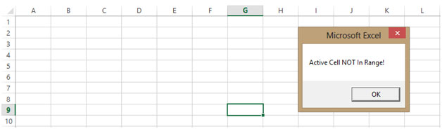
12. Click OK to close the Box
This is how we can determine whether a Cell is within a Range or not using VBA.
![]()
-
#2
Hi and Welcome to the Board.
What specific value are you looking for in «C16»
AND
You want to copy range «F3» to «F last cell» to the first blank cell in «F» ?
-
#3
Hi Michael,
Thanks for the welcome. Basically I have created an invoice sheet (F3:P43) that uses lookups from standard formulas I use based on client, dates, etc, etc to calculate an invoice from other worksheets. What I was doing to keep track of invoices I’ve issued, is to copy and paste the issued invoice values below F43. I’ve ensured that the F column only contains the invoice numbers. So everything below row 43 contains copies of invoices.
I created a macro button to copy and paste values of F3:P43, starting from F44, to the next blank cell in column F. The invoices are always 40 rows long, and each cell in F contains the invoice number it corresponds to.
The reason I want to use VBA is to make sure that I don’t copy and paste duplicates unnecessarily.
-
#4
Ok, now I’m really confused……so what does «cell «C16» have to do with the copy and paste ?
-
#5
Sorry Michael,
I’m a bit tired.
«C16» is the cell/value I want to check/search against «F44:F1000»
IF — the value of «C16» is found in «F44:F100»
THEN — don’t copy and paste
ELSE — copy and paste
END IF
I’ve figured out my copy and paste code. What I’m stuck on, is trying to create a code that will search «F44:F1000» for a value in «C16».
-
#6
Maybe this
Code:
Sub CopyPaste()
Dim lr As Long
lr = Cells(Rows.Count, "F").End(xlUp).Row
    For Each cell In Range("F3:F43")
        If cell.Value = Range("C16").Value Then
           MsgBox "Invoice number already issued."
           Exit Sub
        End If
    Next cell
        Range("F3:P43").Copy
        Range("F" & lr + 1).PasteSpecial Paste:=xlPasteValues
    End Sub
-
#7
Thanks Michael,
That worked great, the only thing I had to change was Line 4, «F3:F43» to «F44:F1000».
But is there away to replace «F44:F1000» I entered to some thing like «F44: («F» & lr + 1)»?
-
#8
MAybe
Code:
Sub CopyPaste()
Dim lr As Long
lr = Cells(Rows.Count, "F").End(xlUp).Row
    For Each cell In Range("F44:F" & lr)
        If cell.Value = Range("C16").Value Then
           MsgBox "Invoice number already issued."
           Exit Sub
        End If
    Next cell
        'Range("F3:F43").Copy ' so should this line change too !!
        Range("F44:F" & lr).copy ' to this ?
        Range("F" & lr + 1).PasteSpecial Paste:=xlPasteValues
    End Sub
-
#9
Perfect Michael, thanks a lot. It’s way too late on this side of the world, but I apprecciate all the help. Time for some sleep.
-
#10
OK, glad it worked. Thanks for the feedback
This tip is about finding out whether a cell is within a range.
- It’s basic set theory… we use VBA’s INTERSECT
What we want to write is some VBA code that tells us whether we have selected a cell within the data table:

Here’s the code we use here:

Explanation
- Using Worksheet_SelectionChange we trap the event that the selection has been changed
- We then set a variable InRange to equal an object returned by the intersect function
- If the interset function doesn’t find an intersect, it returns NOTHING
- We then check whether InRange is equal to NOTHING…
- If it is, the the user has not selected a cell within the range.
- If it’s equal to something, then the range is within MyData
Download sheet to practise how to Find Out If A Cell Is Within A Range in Excel
Training Video on how to Find Out If A Cell Is Within A Range in Excel:
| Attachment | Size |
|---|---|
| find-out-if-a-cell-is-within-a-range.xls | 66 KB |
The IF…THEN statement is one of the most commonly used and most useful statements in VBA. The IF…THEN statement allows you to build logical thinking inside your macro.
The IF…THEN statement is like the IF function in Excel. You give the IF a condition to test, such as “Is the customer a “preferred” customer?” If the customer is classified as “preferred” then calculate a discount amount. Another test could be to test the value of a cell, such as “Is the cell value greater than 100?” If so, display the message “Great sale!” Otherwise, display the message “Better luck next time.”
The IF…THEN can also evaluate many conditions. Like the AND function, you can ask several questions and all the questions must evaluate to TRUE to perform the action. Similarly, you can ask several questions and if any single or multiple of questions are true, the action will be performed. This is like an OR function in Excel.
Task #1 – Simple IF
In this example we will evaluate a single cell. Once we have the logic correct, we will apply the logic to a range of cells using a looping structure.
In Excel, open the VBA Editor by pressing F-11 (or press the Visual Basic button on the Developer ribbon.)
Right-click “This Workbook” in the Project Explorer (upper-left of VBA Editor) and select Insert ⇒ Module.

In the Code window (right panel) type the following and press ENTER.
Sub Simple_If()
We want to evaluate the contents of cell B9 to determine if the value is greater than 0 (zero). If the value is >0, we will display the value of cell B9 in cell C9.
In the Code window, click between the Sub and End Sub commands and enter the following.
If Range("B9").Value > 0 Then Range("C9").Value = Range("B9").Value
If you only have a single action to perform, you can leave all the code on a single line and you do not have to close the statement with an END IF.
If you have more than one action to perform, you will want to break your code into multiple lines like the following example.

When using this line-break style, don’t forget to include the END IF statement at the end of the logic.
Test the function by executing the macro. Click in the code and press F5 or click the Run ![]() button on the toolbar at the top of the VBA Editor window.
button on the toolbar at the top of the VBA Editor window.
The number 45 should appear in cell C9.

If we change the value in cell B9 to -2, clear the contents of cell C9 and re-run the macro, cell C9 will remain blank.

Suppose we want to test the values in Column B to see if they are between 1 and 400. We will use an AND statement to allow the IF to perform multiple tests.
Update the code with the following IF statement.
Sub Simple_If()
	If Range("B9").Value > 0 And Range("B9").Value <= 400 Then
		Range("C9").Value = Range("B9").Value
	End If
End Sub
Test the macro by changing the value in cell B9 to values between 1 and 400 as well as testing values >400 or <=0 (remember to clear the contents of cell C9 prior to each test).
Task #2 – Color all values between 1 and 400 green (Looping Through Data)
Now we want to loop through the values in Column B and perform the test on each value.
Below the existing procedure, start a new procedure named IF_Loop(). Type the following and press ENTER.
Sub IF_Loop()
We want to color all the cells in range B9:B18 green if their cell value is between 1 and 400.
There are many ways to determine the data’s range. For examples of several range detection/selection techniques, click the link below to check out the VBA & Macros course.
Unlock Excel VBA and Excel Macros
The technique we will use is to convert the plain table to a Data Table and use Table References. Table References are great because they automatically expand and contract when data is either added or removed from the table. This keep you from having to update all your formulas and VBA code when data ranges change, which they often do.
Click anywhere in the table and press CTRL-T and then click OK.
We want to restore our original cell colors. Select Table Tools ⇒ Design ⇒ Table Styles (group) ⇒ Expand the table styles list and select Clear (bottom of list).

Rename the table (upper-left) to “TableSales”.

Select cell D7 (or any blank cell) and type an equal’s sign.
=Select cells B9:B18 and note the update to the formula. This contains the proper method for referring to table fields (columns).
=TableSales[Sales]
Highlight the reference in the formula bar (do not include the equal’s sign) and press CTRL-C to copy the reference into memory.

Press ESC to abandon the formula.
Return to the VBA Editor and click between the Sub and End Sub commands in the IF_Loop() procedure.
We want to loop through the sales column of the table. For detailed information on creating and managing looping structures, click the link below.
Excel VBA: Loop through cells inside the used range (For Each Collection Loop)
We want the cell color to change to green if the cell’s value is between 1 and 400. We can use the Interior object to set the Color property to green. Enter the following code in the VBA Editor.
Sub IF_Loop()
	Dim cell As Range
	For Each cell In Range("TableSales[Sales]")
		If cell.Value > 0 And cell.Value <= 400 Then
			cell.Interior.Color = VBA.ColorConstants.vbGreen
		End If
	Next cell
End Sub
Run the updated code to see the results as witnessed below.

The color green is a bit on the bright side. We want a pale green, but we don’t know the color code for pale green. Here is a great way to discover the color of any cell.
Open the Immediate Windows by pressing CTRL-G or clicking View à Immediate Window from the VBA Editor toolbar. This should present the Immediate Window in the lower portion of the VBA Editor.
Select an empty cell and set the fill color to a pale green.

With the newly colored cell selected, click in the Immediate Window of the VBA Editor and enter the following text and press ENTER.
? activecell.Interior.Color
The above command will return the value of the active cell’s fill color. In this case, pale green is 9359529.
Update the VBA code to use the color code for pale green instead of the VBA green.
cell.Interior.Color = 9359529
Run the updated code and notice the colors are a more pleasant pale green.

Task #3 – Color all cells that are <=0 and >400 yellow
Now that we have identified all the numbers between 1 and 400, let’s color the remaining cells yellow. The color code for the yellow we will be using is 6740479.
To add the second possible action will require the addition of an ELSE statement at the end of our existing IF statement. Update the code with the following modification.
  Else
    cell.Interior.Color = 6740479
Run the updated code and notice how all the previously white cells are now yellow.

Task #4 – Negative values will be colored red
We will now update the code to color all the negative valued cells red. The color code for the red we will be using is 192.
To add the third possible action will require the addition of an ELSEIF statement directly after the initial IF statement. Update the code with the following modification.
 ElseIf cell.Value < 0 Then
     cell.Interior.Color = 192
Run the updated macro and observe that all the negative valued cells are now filled with the color red.

Feel free to Download the Workbook HERE.

Published on: August 23, 2018
Last modified: February 21, 2023


Leila Gharani
I’m a 5x Microsoft MVP with over 15 years of experience implementing and professionals on Management Information Systems of different sizes and nature.
My background is Masters in Economics, Economist, Consultant, Oracle HFM Accounting Systems Expert, SAP BW Project Manager. My passion is teaching, experimenting and sharing. I am also addicted to learning and enjoy taking online courses on a variety of topics.
One thing I often found frustrating with VBA is the lack of any easy way to see the values in a range object.
I often use Debug.Print when debugging my VBA and I’d love to just be able to Debug.Print a range like you can with other variables.
But because a range is an object, not a variable, you can’t do that.
One way to see what’s in a range is to step through your code (pressing F8) and when the range is set, you can check the values in the range in the Locals window.
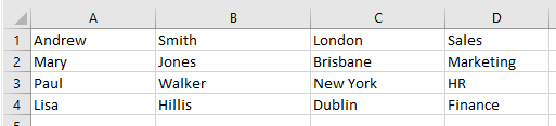
Our range looks like this
How To Open The Locals Window
In the VBA editor go to the View menu and click on Locals Window.
Each time F8 is pressed one line of VBA is executed. When the range MyRange is set, you can see that values appear for it in the Locals window.
By examining the MyRange object you can drill down to see the values in it.
Your browser does not support the video tag.
You can also set a Watch on the MyRange object to examine it in the Watch window, but this is essentially doing the same thing as examining it in the Locals window.
Using both Locals and Watch windows require you to step though code and examine values as the code executes.
If you want to just let the VBA run and see the values in the range printed out to the Immediate window, you need to write some code to do this.
How To Open The Immediate Window
In the VBA editor press CTRL+G, or go to the View menu and click on Immediate Window.
Print Values in Range One by One (Unformatted)
The code shown below will go through each cell in the range and print its value to the Immediate window.
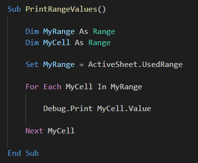
However because we are printing one value at a time, it doesn’t really give you a feel for the structure of the range. That is in this case, that there are 4 values per row/line.
Your browser does not support the video tag.
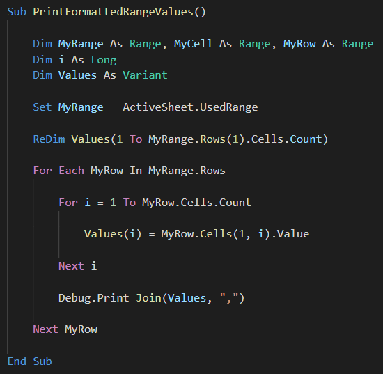
Print Values in Range Row by Row (Formatted)
This next sub stores each value in a row to an array, and then prints out all of these values using the JOIN function to create a string with values separated by a comma.
More on VBA String Functions
This formatted output gives a better representation of the actual structure of your range.
In this format, you can also use the output to write data to a CSV file.
Download Sample Workbook
Enter your email address below to download the workbook containing all the code from this post.
By submitting your email address you agree that we can email you our Excel newsletter.
Здравствуйте. Я не очень разбираюсь с VBA, и мне нужно написать кода типо:
Если значение в столбце F равно «X», то Msgbox1
Иначе (первое условие остается плюс) Если значение в столбце I равно «Y», то Msgbox2
Сейчас у меня код такой:
| Код |
|---|
Private Sub Workbook_Open()
For Each cell In Range("F9:F50")
If cell.Value <= Date And cell.Value <> "" Then
       MsgBox "Attention!" & vbNewLine & "The contract No " & cell.Row & " has expired.", vbOKOnly + vbCritical + vbMsgBoxHelpButton, "Contract expiration"
End If
Next
For Each cell In Range("I9:I50")
If cell.Value <= Date And cell.Value <> "" Then
       MsgBox "Attention!" & vbNewLine & "The contract No " & cell.Row & " is about to expire.", vbOKOnly + vbExclamation, "Contract expiration"
End If
Next
End Sub
|
Соответственно, выскакивают двойные уведомления, от которых я и хочу избавитться.
Спасибо!
п.с. если что, это оповещения об истечении контрактов. столбец F это дата истечения (и если это дата наступила, то контракт истек и вылезает окно «Истек»), столбец I это дата предупреждения (если это дата наступила, то контракт скоро истекает и вылезает окно «Скоро истекает»). Сейчас получается, что если котракт истек, то вылезает и окно «Истек» и окно «Скоро истекает».
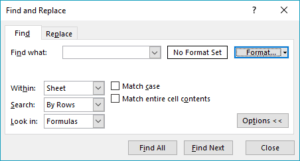
Many times as a developer you might need to find a match to a particular value in a range or sheet, and this is often done using a loop. However, VBA provides a much more efficient way of accomplishing this using the Find method. In this article we’ll have a look at how to use the Range.Find Method in your VBA code. Here is the syntax of the method:
expression.Find (What , After , LookIn , LookAt , SearchOrder , SearchDirection , MatchCase , MatchByte , SearchFormat )
where:
What: The data to search for. It can be a string or any of the Microsoft Excel data types (the only required parameter, rest are all optional)
After: The cell after which you want the search to begin. It is a single cell which is excluded from search. Default value is the upper-left corner of the range specified.
LookIn: Look in formulas, values or notes using constants xlFormulas, xlValues, or xlNotes respectively.
LookAt: Look at a whole value of a cell or part of it (xlWhole or xlPart)
SearchOrder: Search can be by rows or columns (xlByRows or xlByColumns)
SearchDirection: Direction of search (xlNext, xlPrevious)
MatchCase: Case sensitive or the default insensitive (True or False)
MatchByte: Used only for double byte languages (True or False)
SearchFormat: Search by format (True or False)
All these parameters correspond to the find dialog box options in Excel.
Return Value: A Range object that represents the first cell where the data was found. (Nothing if match is not found).
Let us look at some examples on how to implement this. In all the examples below, we will be using the table below to perform the search on.

Example 1: A basic search
In this example, we will look for a value in the name column.
Dim foundRng As Range Set foundRng = Range("D3:D19").Find("Andrea") MsgBox foundRng.AddressThe rest of the parameters are optional. If you don’t use them then Find will use the existing settings. We’ll see more about this shortly.
The output of this code will be the first occurrence of the search string in the specified range.
If the search item is not found then Find returns an object set to Nothing. And an error will be thrown if you try to perform any operation on this (on foundRng in the above example)
So, it is always advisable to check whether the value is found before performing any further operations.
Dim foundRng As Range Set foundRng = Range("D3:D19").Find("Andrea") If foundRng Is Nothing Then MsgBox "Value not found" Else MsgBox foundRng.Address End IfLet us know have a look at the optional parameters. To keep it simple, we will exclude the above error handling in the subsequent examples.
Example 2: Using after
Set foundRng = Range("D3:D19").Find("Andrea", Range("D6"&amp;amp;amp;amp;amp;amp;lt;span data-mce-type="bookmark" style="display: inline-block; width: 0px; overflow: hidden; line-height: 0;" class="mce_SELRES_start"&amp;amp;amp;amp;amp;amp;gt;&amp;amp;amp;amp;amp;amp;lt;/span&amp;amp;amp;amp;amp;amp;gt;)) MsgBox foundRng.AddressOR
Set foundRng = Range("D3:D19").Find("Andrea", After:=Range("D6")) MsgBox foundRng.AddressThe highlighted cell will be searched for
Example 3: Using LookIn
Before seeing an example, here are few things to note with LookIn
- Text is considered as a value as well as a formula
- xlNotes is same as xlComments
- Once you set the value of LookIn all subsequent searches will use this setting of LookIn (using VBA or Excel)
'Look in values Set foundRng = Range("A3:H19").Find("F4", , xlValues) MsgBox foundRng.Address 'Output --&amp;amp;amp;amp;amp;amp;gt; $B$4 'Look in values and formula Set foundRng = Range("A3:H19").Find("F4", LookIn:=xlFormulas) MsgBox foundRng.Address 'Output --&amp;amp;amp;amp;amp;amp;gt; $B$4 'Look in values and formula (as previous setting is preserved) Set foundRng = Range("H3:H19").Find("F4") MsgBox foundRng.Address 'Output --&amp;amp;amp;amp;amp;amp;gt; $H$4 'Look in comments Set foundRng = Range("A3:H19").Find("F4", , xlNotes) MsgBox foundRng.Address 'Output --&amp;amp;amp;amp;amp;amp;gt; $D$4
Example 4: Using LookAt
'Match only a part of a cell Set foundRng = Range("A3:H19").Find("John", , xlValues, xlPart) MsgBox foundRng.Address 'Output --&amp;amp;amp;amp;amp;amp;gt; $D$8 'Match entire cell contents Set foundRng = Range("A3:H19").Find("John", LookAt:=xlWhole) MsgBox foundRng.Address 'Output --&amp;amp;amp;amp;amp;amp;gt; $D$9LookAt setting too is preserved for subsequent searches.
Example 5: Using SearchOrder
'Searches by rows Set foundRng = Range("A3:H19").Find("Sa", , , xlPart, xlRows) MsgBox foundRng.Address 'Output --&amp;amp;amp;amp;amp;amp;gt; $G$4 'Searches by columns Set foundRng = Range("A3:H19").Find("Sa", SearchOrder:=xlColumns) MsgBox foundRng.Address 'Output --&amp;amp;amp;amp;amp;amp;gt; $F$5SearchOrder setting is preserved for subsequent searches.
Example 6: Using SearchDirection
'Searches from the bottom Set foundRng = Range("A3:H19").Find("Alexander", , , , , xlPrevious) MsgBox foundRng.Address 'Output --&amp;amp;amp;amp;amp;amp;gt; $D$18 'Searches from the top Set foundRng = Range("A3:H19").Find("Alexander", SearchDirection:=xlNext) MsgBox foundRng.Address 'Output --&amp;amp;amp;amp;amp;amp;gt; $D$11
Example 7: Using MatchCase
'Match Case Set foundRng = Range("A3:H19").Find("Sa", , , , xlRows, , True) MsgBox foundRng.Address 'Output --&amp;amp;amp;amp;amp;amp;gt; $F$5 'Ignore case Set foundRng = Range("A3:H19").Find("Sa", MatchCase:=False) MsgBox foundRng.Address 'Output --&amp;amp;amp;amp;amp;amp;gt; $G$4
Example 8: Using SearchFormat
When you search for a format it is important to note that the format settings stick until you change them. So, before you use SearchFormat, it is a good practice to always clear any previous formats that have been set.
'Clear any previous format set Application.FindFormat.Clear 'Set the format for find operation Application.FindFormat.Interior.Color = 14348258 'Match format Set foundRng = Range("A3:H19").Find("SA", MatchCase:=True, SearchFormat:=True) MsgBox foundRng.Address 'Output --&amp;amp;amp;amp;amp;amp;gt; $G$15 'Search without matching the format Set foundRng = Range("A3:H19").Find("SA", MatchCase:=True, SearchFormat:=False) MsgBox foundRng.Address 'Output --&amp;amp;amp;amp;amp;amp;gt; $G$4 'Search only for cells of a particular format Set foundRng = Range("B3:H19").Find("*", MatchCase:=True, SearchFormat:=True) MsgBox foundRng.Address 'Output --&amp;amp;amp;amp;amp;amp;gt; $B$3
Example 9: FindNext and FindPrevious
In all the previous examples, we have been looking for just the first occurrence of the search criteria. If you want to find multiple occurrences, we use the FindNext and FindPrevious methods. Both of these need a reference to the last cell found, so that the search continues after that cell. If this argument is dropped, it will keep returning the first occurrence.
'First occurrence Set foundRng = Range("A3:H19").Find("Ms") MsgBox foundRng.Address 'Output --&amp;amp;amp;amp;amp;amp;gt; $C$5 'Find the next occurrence Set foundRng = Range("A3:H19").FindNext(foundRng) MsgBox foundRng.Address 'Output --&amp;amp;amp;amp;amp;amp;gt; $C$10 'Find the previous occurrence again Set foundRng = Range("A3:H19").FindPrevious(foundRng) MsgBox foundRng.Address 'Output --&amp;amp;amp;amp;amp;amp;gt; $C$5
If you are looking to find or list all files and directories in a folder / sub-folder, you can refer to the articles below:
Find and List all Files and Folders in a Directory
Excel VBA, Find and List All Files in a Directory and its Subdirectories
For using other methods in addition to Find, please see:
Check if Cell Contains Values in Excel


