
Private Sub Worksheet_SelectionChange(ByVal Target As Range)
n = 0
While Worksheets(2).Cells(n + 11, 11).Value <> «»
n = n + 1
Wend
On Error GoTo ошибка
For i = 11 To n + 10
If ActiveCell.Offset(-1, 0) = Worksheets(2).Cells(i, 12).Value Then
UserForm3.Show
End If
If ActiveCell.Offset(-2, 0) = Worksheets(2).Cells(i, 12).Value Then
UserForm2.Show
End If
Next
If ActiveCell.Offset(-5, -1).Interior.ColorIndex = 6 Then
UserForm4.Show
End If
If ActiveCell.Offset(-5, 1).Interior.ColorIndex = 27 Then
UserForm4.Show
End If
If ActiveCell.Interior.ColorIndex = 40 Then
UserForm5.Show
End If
If ActiveCell.Offset(-4, 0).Interior.ColorIndex = 15 Then
UserForm4.Show
End If
If ActiveCell.Interior.ColorIndex = 6 Then
UserForm1.Show
End If
If ActiveCell.Interior.ColorIndex = 27 Then
UserForm1.Show
End If
ошибка: MsgBox «Ошибка»
End Sub
Private Sub Worksheet_SelectionChange(ByVal Target As Range)
n = 0
While Worksheets(2).Cells(n + 11, 11).Value <> «»
n = n + 1
Wend
On Error GoTo ошибка
For i = 11 To n + 10
Источник
Notes from the Help Desk

Using Range.Offset in Excel VBA
To select a cell in Excel, you have two basic methods: RANGE and CELLS:
Range works well for hard-coded cells. Cells works best with calculated cells, especially when you couple it with a loop:
Note that your focus does not change. Whatever cell you were in when you entered the loop is where you are when you leave the loop. This is way faster than selecting the cell, changing the value, selecting the next cell, etc. If you are watching the sheet, the values simply appear.
There are times when you are processing a list when you might want to look at the values in the same row, but a couple of columns over. You can accomplish this best with the .Offset clause. You might see the .Offset clause when you record a macro using relative references:
This is both confusing and overkill. Translated into English, it takes the current cell (ActiveCell) and selects the row that is one row down from the current row and in the same column. The “Range(“A1″)” clause is not necessary. So if you want to stay in the current cell and read a value two columns to the right, you could use syntax like the following:
If you are in cell D254, the code above will reference the cell F254 and read its value into the variable strMyValue. This is far more efficient than selecting the cell two columns to the right, processing your data, then remembering to select two columns to the left and continue.
If you want to offset to a column to the left of you or a row above you, use a negative number. If you are in cell G254, the code ActiveCell.Offset(-3,-2).Select will select E251 (3 rows up and 2 columns left).
You can loop through a list much more efficiently with Offset. It is easier to program and way faster to execute.
You would probably want to format the salary for currency, but this is the general idea.
Comments
Using Range.Offset in Excel VBA — 48 Comments
I am removing rows from worksheet A to worksheet B to be archived. Somewhere in my code it does not continue the offset, everytime i remove it replaces the current line. I use A1 as my reference point from worksheet B. Here is the code
Range(“B2”).Select
Selection.Copy
Sheets(“Removed from wait list 2015”).Select
Range(“A1”).Select
ActiveCell.Offset(1, 0).Select
ActiveSheet.Paste
Sheets(“Wait List”).Select
Range(“C2”).Select
Application.CutCopyMode = False
Selection.Copy
Sheets(“Removed from wait list 2015”).Select
Range(“A1”).Select
ActiveCell.Offset(1, 1).Select
ActiveSheet.Paste
Sheets(“Wait List”).Select
Range(“D2”).Select
Application.CutCopyMode = False
Selection.Copy
Sheets(“Removed from wait list 2015”).Select
Range(“A1”).Select
ActiveCell.Offset(1, 2).Select
ActiveSheet.PasteSpecial
Sheets(“Wait List”).Select
Range(“E2”).Select
Application.CutCopyMode = False
Selection.Copy
Sheets(“Removed from wait list 2015”).Select
Range(“a1”).Select
ActiveCell.Offset(1, 3).Select
ActiveSheet.Paste
Sheets(“Wait List”).Select
Range(“F2”).Select
Application.CutCopyMode = False
Selection.Copy
Sheets(“Removed from wait list 2015”).Select
Range(“A1”).Select
ActiveCell.Offset(1, 4).Select
ActiveSheet.Paste
Range(“A1”).Select
ActiveCell.Offset(1, 8).Select
Application.CutCopyMode = False
ActiveCell.FormulaR1C1 = Date
Range(“A1”).Select
ActiveCell.Offset(1, 9).Select
ActiveCell.FormulaR1C1 = Application.UserName
Sheets(“Wait List”).Select
Rows(“2:2”).Select
Selection.Delete Shift:=xlUp
When you are deleting with Range Offset, it is better to start on the last row and delete/cut it, then move up one row and work with that. When you cut a row, you need to make sure to move to the next row and you can control it better from the bottom up.
Also, rather than hardcode your cell references, use loops:
for i = LastRow to FirstRow Step -1
cells(i,colnumber).select
cut/copy as you are doing
switch to the “removed” sheet
paste
move down one row
switch back to the “wait List” sheet
next i
i will select the next row up and work with it. If necessary, sort the “Removed” list after you are done.
Thank John Walkenbach for the tip on moving up one row.
I need a code for example
If Range(“A2”).Select
Range(Selection, Selection.End(xlDown)).Select
Selection.Copy
Range(“A11”).Select
ActiveSheet.Paste
Here the range is mentioned as A11 for pasting the data if i continue it for next day it is pasting the data on A11 itself but it should select the next 11th line for ex A22 and if i do for the third day the data should be pasted on A33 etc….
Try substituting the following for your Range(“A11”).Select statement:
This will add 11 to whatever row you are in and move you down 11 rows.
Also, not sure why there is an IF in Row 1. If this is part of a larger code section, no worries. Otherwise, just get rid of it since there is no corresponding END IF.
I’m looking for code that finds the value “NOF” in a column then copies that row and the 10 rows above and below into a new sheet and prints it.
such as in column J, the cell J100 contains “NOF”
i want to print all columns (A:K) for rowns 90 throught 110.
i need to code to read through this giant work book and print a page for the many instances of “NOF”
Hey,
I want to copy one range (A2:A9) from one sheet to another with an additional empty space(column) between each cell.
E.G – in sheet2, – B2 = sheet1 A2, B3 (empty), B4 = sheet1 A3, B5 (empty), etc.
While also adding the range to the next available row on the second sheet.
I’ve got the code for X1row but not the offset.
Please help.
A bunch of ways to do it. Here’s a quick and dirty one. You copy the current cell + j (as j goes from 0 to 7), then switch to the second sheet, and offset by 2 each times (i = 1 to 14 Step 2 – add 2 to the loop control variable).
I’d probably virtualize the cell references rather than hardcode A2:A9, but this is a fast fix:
Sub MoveIt()
Dim intRow As Integer
Dim intCol As Integer
Dim i As Integer
Dim j As Integer
intRow = 2
intCol = 1
j = 0
Range(“A2”).Select
For i = 0 To 14 Step 2
Worksheets(2).Cells(intRow + i, intCol + 1).Value = ActiveCell.Offset(j, 0).Value
j = j + 1
Next i
Hi,
I need to extract data from the table of a website and put those values in the reverse order in a specific row,column of my excel sheet. Here’s my code:
Set Table = appIE.document.getElementsByClassName(“table4”)
r = 52
c = 10
For Each itm In Table
Worksheets(1).Range(“F52”).Offset(r, c).Value = itm.innerText
End If
Next itm
I need this code to repeat continuously after every use. After I search the keyword I am looking for, I want it to go to the next line and when I search again, I want it to save what I had originally searched for, and continue just like that.
Here is the code:
Sub Test2()
Dim myWord$
myWord = InputBox(“What key word to copy rows”, “Enter your word”)
If myWord = “” Then Exit Sub
Application.ScreenUpdating = False
Dim xRow&, NextRow&, LastRow&
NextRow = 2
LastRow = Cells.Find(what:=”*”, After:=Range(“A1”), SearchORder:=xlByRows, SearchDirection:=xlPrevious).Row
For xRow = 1 To LastRow
If WorksheetFunction.CountIf(Rows(xRow), “*” & myWord & “*”) > 0 Then
Rows(xRow).Copy Sheets(“Jannah”).Rows(NextRow)
NextRow = NextRow + 1
End If
Next xRow
Application.ScreenUpdating = True
MsgBox “Macro is complete, ” & NextRow – 2 & ” rows containing” & vbCrLf & _
“”” & myWord & “”” & ” were copied to Jannah.”, 64, “Done”
End Sub
I see some issues with your code.
First, you shouldn’t copy the entire row, just the cells you want. Not: rows(xRow).copy but Range(cells(xRow,1),cells(xrow,#)).copy
Second, I am not clear about what you mean repeat continuously. Do you mean that the next time you run it, it will keep the previous copies and continue? You’ll need to have a marker of some sort – save the row copied from to Jannah and use that as a start row+1 is one way.
Also: Sheets(“Jannah”).Rows (nextrow) doesn’t seem to work. I replaced it with:
Sheets(“Jannah”).Activate
ActiveSheet.Paste
Application.CutCopyMode = False
nextrow = nextrow + 1
What version of VBA are you using? Some interesting constructions there. I’d go about them differently, but yours work.
I’m trying to run a series of macros down a list of values.
First step-change cell value (based on dropdown list-lookup)
This triggers a macro (on value change) that changes the filters on several pivot tables “vChange()”
Second step-“Print_toPDF()” macro that I have assigned to a button that prints a pdf of my template and names it based on a dynamic cell
I planned to use the call statement for both macros, but I can’t figure out how to set up the loop to change the cell value (the cell value needs to change for the value change macro and because I’ve set up several vlookups with that cell).
Any help would be appreciated.
Hi Admin, Here is my need ! Kindly let me know your feedback .
Sheet 2 have column A,B and C and sheet 1 need to be updated in the below format
Sheet(1) column B2-B9 cell should be updated from Sheet(2) column B2
Sheet(1) column C2 cell should be updated from Sheet(2) column C2
Sheet(1) column J9 cell should be updated from Sheet(2) column C2
and
Sheet(1) column B10-B17 cell should be updated from Sheet(2) column B3
Sheet(1) column C10 cell should be updated from Sheet(2) column C3
Sheet(1) column J17 cell should be updated from Sheet(2) column C3
and
Sheet(1) column B18-B25 cell should be updated from Sheet(2) column B4
Sheet(1) column C18 cell should be updated from Sheet(2) column C4
Sheet(1) column J25 cell should be updated from Sheet(2) column C4
etc….. This range is uniform and need to generate close to 1000 nos.
Awaiting response.. Thanks !
Not sure what you are asking for. The general code follows. You should be able to put it in loop.
Dim intRow1, intRow2, intCol1, intCol2 As Integer
intRow1 = 5
intCol1 = 2
‘C7
intRow2 = 7
intCol2 = 3
Worksheets(“Sheet1”).Cells(intRow1, intCol1).Value = Worksheets(“Sheet2”).Cells(intRow2, intCol2).Value
HI Admin,
Looking to code a search of a row of cells that will sum the values of the cells containing the value 2. I need to find the first cell value with value 2 then sum cells to the right until cell 2. Cell value will be either zero or 2 both a result of a formula in the cell. Test if the sum of the cells with values 2 => X and if so return a message “yes you reached your goal” , if not continue checking until a total of 95 cells to the right from the starting cell have been checked.
I have got this far and now stumped.
Dim x As Range
Dim i As Long
Dim iVal As Integer
On Error Resume Next
Set x = Application.InputBox(prompt:=”Please click on the spot to start counting from “, Type:=8)
‘ Application.ScreenUpdating = False
If Not x Is Nothing Then
Range(x.Address).Select
Range(x.Address).Offset(996).Select
Selection.Resize(Selection.Rows.Count + 0, Selection.Columns.Count + 672).Select
Set rngMyRange = Selection
For i = 1 To 95
i = i + 1
Do
Range(rngMyRange).Value = Selection.Value + 1
iVal = Application.WorksheetFunction.CountIf((Selection), “2”)
ActiveCell.Offset(0, 1).Select
‘ Set Do loop to stop when an empty cell is reached.
Loop Until Selection.Value = 0
End If
On Error GoTo 0
‘ Application.ScreenUpdating = True
End SubSub Find24hours_Rest()
Dim x As Range
Dim i As Long
Dim iVal As Integer
On Error Resume Next
Set x = Application.InputBox(prompt:=”Please click on the spot to start counting from “, Type:=8)
‘ Application.ScreenUpdating = False
If Not x Is Nothing Then
Range(x.Address).Select
Range(x.Address).Offset(996).Select
Selection.Resize(Selection.Rows.Count + 0, Selection.Columns.Count + 672).Select
Set rngMyRange = Selection
For i = 1 To 15
i = i + 1
Do
Range(rngMyRange).Value = Selection.Value + 1
iVal = Application.WorksheetFunction.CountIf((Selection), “2”)
ActiveCell.Offset(0, 1).Select
‘ Set Do loop to stop when an empty cell is reached.
Loop Until Selection.Value = 0
End If
On Error GoTo 0
‘ Application.ScreenUpdating = True
Hello Admin. See if you can help me out with this one.
I have a file with attribute names as headers and applicable values in the columns beneath each header. Rows mean nothing to me here. I need to remove all duplicate values and sort, per column.
I thought the easiest thing to do would be to record a macro on one column, and then run the macro on the each of the remaining columns .. but that ain’t working.
Can you help? Does this even make sense?
I’d like to ask for your help. I have workbook calendar type workbook.
It looks like something like this.
A col. B col. D col. E col. F col.
1 Startdate Starttime Enddate Endtime Title etc….
2 2017.11.09 8:00 2017.11.09 12:00 Dosthing
3 2017.11.12 9:00 2017.11.13 15:00 ETC
4 .. .. …. .. ..
5
I need a button, – on a different worksheet – which “jumps” to A5. If i fill a new row then A6 etc…
Thanks in advance for your help!
If you’re interested, i can share my workbook with you.
Please assist
I am creating a xml document with header and detail data.
I have two columns in Excel
Column A = Customer and Column B equals Stockcode
So I need 2 loops. The fist loop to only select the customer code once as this is the header information and the second loop to select each stockcode for the customer
Your assistance will be greatly appreciated
Many thanKS
A B
Customer code Stockcode
201 123ex
201 124ex
201 125 ex
203 123ex
203 124ex
I want to copy cells A2 and B2 from sheet 2 on to cells C12 and C13 in sheet 1. Then Copy Cells A3 and B3 from sheet 2 to cells C12 and C13. Then do this until there the last row in sheet 2. Below is what I have been able to do so far.
Put it in a loop
Dim strSheet1Value1 as string
Dim strSheet1Value2 as string
Worksheets(“Sheet1”).Range(“C12”).Select
Worksheets(“Sheet2”).Range(“A2”).Select
Worksheets(“Sheet1”).activate
While ActiveCell.Value <> “”
strSheet1Value1 = ActiveCell.Value
strSheet1Value2 = activeCell.offset(0,1).value
ActiveCell.Offset(1,0).Select
Worksheets(“Sheet2”).activate
ActiveCell.Value = strSheet1Value1
activeCell.Offset(0,1).value = strSheetValue2
ActiveCell.Offset(1,0).Select
Worksheets(“Sheet1”).Activate
Wend
Are you sure you mean to always put the value in C12 and C13? If you do, you will only get the last value in your list.
How can I return the value that is always 3 columns to the right of the found value?
Use offset. Say you find the value using ActiveCell:
dim strThreeColValue as string
The offset will take the current cell and look 0 columns and 3 columns to the right and return the value. The ActiveCell won’t change. You can use a loop to iterate through all your values:
While ActiveCell.value <> “”
strThreeColValue = activecell.offset(0,3).value
‘do whatever else you need to
ActiveCell.Offset(1,0).Select ‘move down one row. Without this, you have an endless loop
Wend
I’m new to VB Excel. I have a form where i would like the user to click the button and each click populates the value “Yes” every time the button is clicked. However, what my code is doing is one click and every cell is populated with Yes. I also have a no button… it’s doing the same thing. Once click and all field are populated with “No”. Would you be able to help me fix the code so that in the each click populates only one entry of “Yes” or only one entry of “No”? Thank you for your time.
If Selection.Address = (“$B$15:$D$15”) Then
ActiveCell.Value = “Yes”
ActiveCell.Offset(1, 0).Range(“A1”).Select
End If
If Selection.Address = (“$B$16:$D$16”) Then
ActiveCell.Value = “Yes”
ActiveCell.Offset(1, 0).Range(“A1”).Select
End If
If Selection.Address = (“$B$17:$D$17”) Then
ActiveCell.Value = “Yes”
ActiveCell.Offset(1, 0).Range(“A1”).Select
End If
If Selection.Address = (“$B$18:$D$18”) Then
ActiveCell.Value = “Yes”
ActiveCell.Offset(1, 0).Range(“A1”).Select
End If
If Selection.Address = (“$B$19:$D$19”) Then
ActiveCell.Value = “Yes”
ActiveCell.Offset(1, 0).Range(“A1”).Select
End If
If Selection.Address = (“$B$20:$D$20”) Then
ActiveCell.Value = “Yes”
ActiveCell.Offset(1, 0).Range(“A1”).Select
End If
If Selection.Address = (“$B$21:$D$21”) Then
ActiveCell.Value = “Yes”
ActiveCell.Offset(1, 0).Range(“A1”).Select
End If
The problem is that your code updates B15:D15, then moves down a row. The next line of code tests whether the range is B16:D16, which it now is. So your code then executes that section, moves down and tests B17:D17, which is now true. So your code will execute every test in turn.
Since the code always puts “Yes” in the selected cell, you can simply use the ActiveCell.Value = “Yes” and the ActiveCell.Offset line rather than test for where you are, since wherever you are, you are entering yes.
If your code does more than you are showing, try using a SELECT CASE statement:
Select Case Selection.Address
Case «$B$15:$D$15: ActiveCell.value = «Yes»
Case «$B$16:$D$16: ActiveCell.value = «yes»
‘.
End Select
Or at least use IFElse statements:
If Selection.Address = (“$B$15:$D$15”) Then
ActiveCell.Value = “Yes”
ActiveCell.Offset(1, 0).Range(“A1”).Select
Else If Selection.Address = (“$B$16:$D$16”) Then
ActiveCell.Value = “Yes”
ActiveCell.Offset(1, 0).Range(“A1”).Select
.
End If
hi
i need help in the following :
This is my criteria .Whenever i move a row down from Row 1 ,C2 and E2 will auto return with yes.
Problem is i always need to go to row 1 to execute it. i want it to be whatever cell i am in , i execute where i am to leave the loop .
Public Sub InsertRow()
ActiveCell.Offset(1, 0).Rows(“1:1”).EntireRow.Insert Shift:=xlDown
Range(“C2”).Value = “no”
Range(“E2”).Value = “no”
End Sub
It is unclear what you are asking. The first row inserts a row below the Active Cell, so I don’t understand why you have to go to Row 1. There is no loop in your code sample, so I don’t know what else you are doing that might affect the Active Cell. More information please.
Sorry for the confusion .
-I have 5 column in the excel sheet (A TO E). C1 and E1 will be inputted as “YES”. A1 ,B1 and D1 will not be touched as they are general information.
-I want to copy cell C1 to C2 as “YES” , E1 to E2 as “YES” at the same time ,whenever I insert a new row . then do this until there the last row in sheet is .
Sub Macro1()
r = ActiveCell.Row
Cells(r + 1, 3).EntireRow.INSERT
Cells(r, 3).Copy Destination:=Cells(r + 1, 3)
End Sub
Current problem from this formula is, I only can copy Column C down the row.
I have limited experience with VB however I’m trying to combine information from 2 worksheets to reconcile payment information.
I have a “PayPal” worksheet and an “Accounts Data” worksheet – I’m trying to generate code to Select the first “Customer Number” from column A in the PayPal sheet (A2) then copy the contents from cells E through H in that row, then swap to the Accounts Data sheet, search for a matching Customer Number (now headed “P.O.#” Column A) and Paste the data into L through O in that row. Then repeat until the end of the data in the PayPal sheet.
I have made up a few Macros to rearrange the data and to exclude redundant information, but I’ve been grappling with this Search/Copy/Match/Paste loop and can’t get my head around it.
Any assistance would be greatly appreciated.
I would use a VLOOKUP to make the find and paste easier. In the Accounts Data sheet, enter a VLOOKUP to search for the customer data in Paypal, then return a value from that list. Add multiple VLOOKUPs, one for each column you want to bring in. Then, copy them down. When you are done, you can do a Paste Special Values to get rid of the VLOOKUP and get just the values in place. Use an IFERROR statement to capture a “Not Found” situation.
You can put this in a macro, including adding the VLOOKUP, if you want. I would create the VLOOKUPs in the first row, turn on R1C1 style (Options|Formulas) and copy the resulting formula. Put it in quotes in an ActiveCell.Offset(0,#).FormulaR1C1 statement.
You can use the Find option, but you need a Boolean variable, bolFound, to assign to the Find and then test if bolFound = True, then you have the right row. This is going to be a little trickier, I think.
Thanks for this info and suggestion.
After lots of reading, research, trial and lots of errors – I found VLOOKUP and it worked well and is much more simple that other ideas I had.
I have collated the stages of creating the final report into 3 separate macros, which I will look at cleaning up a little later – just for now I’m happy I have a Reconciliation Report I can work with.
I’m not familiar with R1C1 or IFERROR statements, but it will give me something to research and see how I can apply them.
Currently I suspect I have a problem with the Copy Down process I used in recording the macro – I used a double click to copy the VLOOKUP formula down the column to the end of the data, but it has hard coded the range (H3:H100) into the macro. I wasn’t sure how to do this otherwise. It will become an issue as the number of entries increases past 97.
Thanks for your help.
The hard-coded range was probably put in there when you recorded it. There are a number of ways to fix this, with macros and without, but the simplest is to change the range to 200 or 300 and then copy it down.
The R1C1 style won’t be necessary if you are doing the copying manually. The IFERROR function will display a value if the formula you want to use results in an error. For example, IFERROR([vlookup formula here],””) will display a blank if the vlookup results in an #N/A! error if the ID is not found. You could change the “” to 0 if you want a number you can use.
Later on, after you’ve used this for a while, you could look into creating a macro for the whole thing.
I have spread sheet with Column titles are Names Person A, Person B. Column has repeat values e.g. Late, Early, Day, Rest, Etc.
Column A is Weekday e.g. Monday, tues etc. and Column B is Date.
Column C to P have various Person Name as title. Row 2 to 30 have various shift pattern with value of Early, day, Rest.
I want to create table with Macro where Date is Column Title and Shift Type is Row title. e.g. it puts Name of person from column C for Early (if marked as early) if not goes to next column to search for Early) if there are multiple early I want it to populate it too.
I will appreciate your help thank you
I am not sure what you are asking. Can you be more specific about what each column and row contains? Thanks.
I have an Excel template with columns A to C but col B has formula in it and I want my Access table to export data only from col A and C, but skip col B.
Please suggest the code that can do this transfer. Thank you.
You mean you want to export Col A and C and then import it into Access? Can you create an import mask in Access to ignore column B? Otherwise, I would copy A and C to a new sheet, then save that sheet as a Tab Delimited File and import that into Access.
Sorry for the confusion. I want to export Col A from Access table to col A into Excel template. And Col B & C from Access to Col C & D in Excel worksheet. This just a sample there is a lot more columns involved in that process. Basically I have a complicated formula in Col B in Excel template that I don’t want overwrite when moving data from Access to Excel and would like to automate this process using VBA code. Thank you.
The simplest is to export each field directly and skipping B. Read the value into a variable in Access. You’ll need to create an instance of the other application (Access if you are in Excel or Excel if you are in Access). Once you do:
[switch to Access, read the value into the variable]
[Switch to Excel]
[assume you are using a loop to enter multiple rows and the loop control variable is “i”]
Cells(i,1).value = [variable name]
[Switch back to Access and read the next value into the variable]
Switch back to Excel]
Cells(i, 3).VALUE = [variable name]
[keep doing this for all of your values]
At the end of the row, the loop will increment i so you enter the next row.
There are probably sexier ways to do this, but this is simple and reliable and unless you have 100,000 rows, the performance is fine.
I need a VBA Code which will copy Above Cell value Range E2: G till the previous columns have value and once Previous coulmn cell value come blank, it stop copying.
I am not sure what you are asking. A While loop, While ActiveCell.Value <> “” will continue copying until you hit a blank row. Make sure to add an ActiveCell.Offset(1,0).Select statement to the end of the While look to move the cell cursor. Otherwise, it will stay on the current cell forever.
I am filling a column (from E18 to E90) with cell values from other worksheets. It is all working fine but when it reaches E90 I would like excel to continue filling cells in column L (Offset(0,7)).
With the following code, where would I add the Offset code to make it work?
For rep = 1 To (Worksheets.Count)
If Worksheets(rep).Cells(27, 2).Value = “Open” Or Worksheets(rep).Cells(27, 2).Value = “Closed” Or Worksheets(rep).Cells(27, 2).Value = “Partly-resolved” Or Worksheets(rep).Cells(27, 2).Value = “(Non-issue)” Then
b = Worksheets(“Issue Tracker”).Cells(Rows.Count, 5).End(xlUp).Row
Worksheets(“Issue Tracker”).Cells(b + 1, 5).Value = Worksheets(rep).Cells(27, 2).Value
Any help would be much appreciated.
I would add the following code. You are accomplishing your task without Offset so continue to do so.
if activecell.row > 90 then
intCol = 7
else
intCol = 5
end if
b = Worksheets(“Issue Tracker”).Cells(Rows.Count, intCol).End(xlUp).Row
Hi Admin, I’m kind of new to VBA programming and with some google help I have reached to the code below. But the VBA-code save the files as *.xls files and I would want to save it as *.xlsx files since I’m running on Excel2016. If I only replace the *.xls with *.xlsx the saved files are corrupt and empty! I can handle that even if it is *.xls files, but the more important which I hope you could guide me on following:
I have let say nine *.xls files and I want to move one column from each *.xls file to a different file (we call it “joined_tst.xls”). So in this file nine columns from B is populated with data from each *.xls file. I tried with below code, but when it reaches “Windows(“joined_tst.xls”).Activate” it give the alert code and stop the process. Could you please suggest why it does not proceed. Also could you please suggest how I can move one column forward by each file. (In highlighted code below I want it to be B1 from first file, C1 from second file, D1 from third and so one in joined_tst.xls file).
Thank you,
Sub Macro4()
‘
‘ Macro4 Macro
‘
‘Private Sub CommandButton1_Click()
Dim MyFolder As String
Dim myfile As String
Dim folderName As String
With Application.FileDialog(msoFileDialogFolderPicker)
.AllowMultiSelect = False
If .Show = -1 Then
folderName = .SelectedItems(1)
End If
End With
myfile = Dir(folderName & “*.txt”)
Do While myfile “”
Workbooks.OpenText Filename:=folderName & “” & myfile
Cells.Select
Selection.Replace What:=”.”, Replacement:=”,”, LookAt:=xlPart, _
SearchOrder:=xlByRows, MatchCase:=False, SearchFormat:=False, _
ReplaceFormat:=False
Columns(“E:E”).Select
Selection.FormatConditions.AddTop10
Selection.FormatConditions(Selection.FormatConditions.Count).SetFirstPriority
With Selection.FormatConditions(1)
.TopBottom = xlTop10Top
.Rank = 1
.Percent = False
End With
With Selection.FormatConditions(1).Interior
.PatternColorIndex = xlAutomatic
.Color = 10498160
.TintAndShade = 0
End With
Selection.FormatConditions(1).StopIfTrue = False
Selection.Copy
‘Windows(“joined_tst.xls”).Activate
Range(“B34”).Select
Application.CutCopyMode = False
ActiveCell.FormulaR1C1 = “PC2”
‘save as excel file
ActiveWorkbook.SaveAs Filename:=folderName & “” & Replace(myfile, “.txt”, “.xls”)
‘use below 3 lines if you want to close the workbook right after saving, so you dont have a lots of workbooks opened
Application.DisplayAlerts = False
ActiveWorkbook.Close
Application.DisplayAlerts = True
myfile = Dir
Loop
End Sub
‘End Sub
First, you need to understand XLS vs XLSX /XLSM. The old XLS format allows macros. The new format, XLSX, does not. If you save a file with macros as an XLSX file, it will strip the macros out. Save it as a macro-enabled workbook, XLSM format.
The error message may be because the joined_tst.xls isn’t open. It must be open for you to refer to it as a Window.
The code you posted has a bunch of code in it to convert . to , and to add conditional formatting. To do the copy, I would use something like this:
dim i as Integer
dim strFileName as string
file.open filename:=»joined_tst.xls”
strfilename = input(«what is the name of the first file?»)
for i = 2 to 10
file.open filename:=strfilename
cells(1,i).EntireColumn.select ‘This selects column b for the first file
worksheets.copy
workbooks(«joined_tst.xls”).activate
cells(1,i).select ‘selects B1 in the first file
selection.paste
application.cutcopypaste = False
workbooks(strfilename).close
strfilename = input(«what is the name of the next file?»)
next i
You may need to tweak this. It will open each file and since you are using a variable to select the column, it will move one column over each time you go through the loop. It starts at 2 to start at column B simply.
Hello Admin,
I need to export Col A from Access table to col A into Excel template. And Col B & C from Access table to Col C & D in Excel template. This just a sample there is a lot more columns involved in that process. Basically I have a complicated formula in Col B in Excel template that I don’t want overwrite when moving data from Access to Excel and would like to automate this process using VBA code. Please help. Thank you.
I have taken a few college courses related to Excel and C sharp, looks like I took the wrong coding language course because I cannot figure out how to write a macros to save my life! I understand loops etc. it is the language that evades me. I desperately need a macros that can highlight 1 entire row of data AFTER the user has entered data into EVERY cell within the specified row/range. Conditional formatting is not working…I have only been able to highlight each cell directly after the user enters data into individual cells (leaving blanks where data is missing which I do not want…) or highlight the entire row based on 1 cells value but this too includes the blank cells which is not what I am going for. Simply put, I need it to highlight the row once the user has entered values/string in each cell and NOT a minute sooner. The idea is to visually check off that a job is complete and that is indicated by every cell in that row containing data. Any help you can provide is greatly appreciated.
I would do a conditional format rather than a macro:
1. Select the entire range you want to format. Include blank rows if you must.
2. Add a conditional format using a formula. It is painful to create the formula in the first place. You add the formula as though you were entering it into the first cell. The formula will be replicated for every cell in the highlighted range.
3. For example, the formula for “non-blank cells” A3 through I3 is
=AND($A3<>“”,$B3<>“”,$C3<>“”,$D3<>“”,$E3<>“”,$F3<>“”,$G3<>“”,$H3<>“”,$I3<>“”)
Notice the absolute columns. They are needed to make sure the proper cells are evaluated in every instance.
4. Set the conditional format.
5. Excel will apply the formula to every cell in the range. Only ranges with all cells filled in will be colored. So if A5:I5 are filled in, the conditional format will apply to A5:I5. If A6:I6 are mostly filled in, the cells remain normal.
Actually, rereading your question, you want to use the macro and move to the next cell. The code would be:
activecell.value = [result of the macro]
activecell.offset.(1,0).select
while activecell.value <> «»
activecell.offset(1,0).select
wend
This puts the calculation into the current cell, then moves down one row. While the contents of the new row are not blank, it keeps moving down. If you know the next row is blank, all you need is the activecell.offset(1,0).select to move to the next row.
If you want to process a range of cells, this is the way to do it.
There are a lot of ways to do this. One way is to use a construct like this. Say you want to put a value in Column A:
Sub NextRow
dim i as integer
dim j as integer
while [Not done — you set the condition]
cells(i,j).value = i*j [or some other calculation]
i=i+1
wend
The statement cells(i,j).value will put a value in the cell A1, then increase i (the row) by one. The next time the loop runs, it will put the value in A2. And then A3 etc. You have to modify the example to add the test in the While line (while some condition is true). You have to do the calculation or processing and put the result in Cells(i,j).value [cells( row #, column #)]. Depending on the processing, it may be easier to put the result into a variable, then put the value of the variable in the Cells(i,j).value.
Источник
Adblock
detector
To select a cell in Excel, you have two basic methods: RANGE and CELLS:
Range ("A1").Select
Range("RangeName").Select
Cells(3, 4).Select 'Selects Row 3, Column 4, i.e. cell D3
Range works well for hard-coded cells. Cells works best with calculated cells, especially when you couple it with a loop:
For i = 1 to 10
     Cells(i, 1).value = i   ' fill A1 through A10 with the value of i
Next i
Note that your focus does not change. Whatever cell you were in when you entered the loop is where you are when you leave the loop. This is way faster than selecting the cell, changing the value, selecting the next cell, etc. If you are watching the sheet, the values simply appear.
There are times when you are processing a list when you might want to look at the values in the same row, but a couple of columns over. You can accomplish this best with the .Offset clause. You might see the .Offset clause when you record a macro using relative references:
ActiveCell.Offset(1, 0).Range("A1").Select
This is both confusing and overkill. Translated into English, it takes the current cell (ActiveCell) and selects the row that is one row down from the current row and in the same column. The “Range(“A1″)” clause is not necessary. So if you want to stay in the current cell and read a value two columns to the right, you could use syntax like the following:
strMyValue = ActiveCell.Offset(0,2).Value
If you are in cell D254, the code above will reference the cell F254 and read its value into the variable strMyValue. This is far more efficient than selecting the cell two columns to the right, processing your data, then remembering to select two columns to the left and continue.
If you want to offset to a column to the left of you or a row above you, use a negative number. If you are in cell G254, the code ActiveCell.Offset(-3,-2).Select will select E251 (3 rows up and 2 columns left).
You can loop through a list much more efficiently with Offset. It is easier to program and way faster to execute.
While ActiveCell.Value <> ""
    strFirstName = ActiveCell.Value

    strLastName = ActiveCell.Offset(0,1).Value

    dblSalary = ActiveCell.Offset(0,2).Value

    ActiveCell.Offset(0,2).Value = dblSalary * 1.05 'give a 5% raise

    MsgBox(strFirstName & " " & strLastName & ": Your new salary is " & dblSalary)

    ActiveCell.Offset(1,0).Select

Wend
You would probably want to format the salary for currency, but this is the general idea.
In this Article
- ActiveCell.Offset Properties and Methods
- ActiveCell.Offset Syntax
- ActiveCell.Offset..Select
- Using Range Object with Activecell.Offset Select
- Alternatives to ActiveCell
This tutorial will demonstrate how to use Activecell Offset in VBA.
The ActiveCell is a property of VBA that represents the cell address of the active cell in your worksheet. If the cursor is positioned in cell A1 then the ActiveCell property in VBA will return the cell address of “A1”. The are a number of properties and methods that are connected to the ActiveCell. In this article we are concentrating on the ActiveCell.Offset method.
ActiveCell.Offset Properties and Methods
Activecell.Offset has a number of properties and methods available to be programmed with VBA. To view the properties and methods available, type the following statement in a procedure as shown below, and press the period key on the keyboard to see a drop down list.
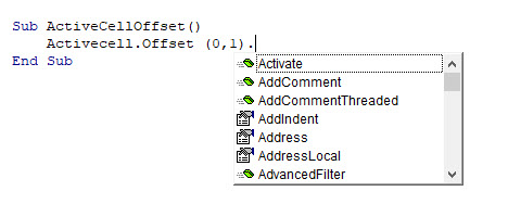
Methods are depicted by the green method icon, and properties by the small hand icon. The properties and methods for the ActiveCell.Offset method are the same as for the ActiveCell method.
ActiveCell.Offset Syntax
The syntax of ActiveCell.Offset is as follows
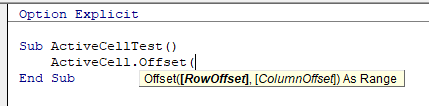
where the RowOffset and ColumnOffset is the number of rows to offset (positive numbers for down, negative number for up) or the number of columns you wish offset (positive numbers offsets to the right, negative number to the left).
ActiveCell.Offset..Select
The Activecell.Offset..Select method is the most commonly used method for with Activecell.Offset method. It allows you to move to another cell in your worksheet. You can use this method to move across columns, or up or down rows in your worksheet.
To move down a row, but stay in the same column:
Activecell.Offset(1,0).SelectTo move across a column, but stay in the same row:
Activecell.Offset (0,1).SelectTo move down a row, and across a column:
Activecell.Offset (1,1).SelectTo move up a row:
Activecell.Offset(-1,0).SelectTo move left a column:
Activecell.Offset(0,-1).SelectIn the procedure below, we are looping through a range of cells and moving down one row, and across one column as we do the loop:
Sub ActiveCellTest()
  Dim x As Integer
  Range("A1").Select
  For x = 1 To 10
   ActiveCell = x
   ActiveCell.Offset(1, 1).Select
  Next x
End Sub
The result of which is shown in the graphic below:
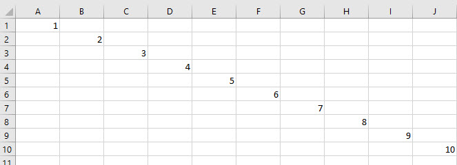
The Loop puts the value of i (1-10) into the Activecell, and then it uses the Activecell.Offset property to move down one row, and across one column to the right – repeating this loop 10 times.
Using Range Object with Activecell.Offset Select
Using the Range Object with the active cell can sometimes confuse some people.
Consider the following procedure:
Sub ActiveCellOffsetRange()
  Range("B1: B10").Select
  ActiveCell.Offset(1, 1).Range("A1").Select
End Sub
With the ActiveCell.Offset(1,1.Range(“A1”), the Range(“A1”) has been specified. However, this does not mean that cell A1 in the sheet will be selected. As we have specified the Range(“B1:B10”), cell A1 in that range is actually cell B1 in the workbook. Therefore the cell will be offset by 1 row and 1 column from cell B1 NOT from cell A1.
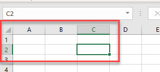
Therefore, the Range(“A1′) in this instance is not required as the macro will work the same way with it or without it.
Alternatives to ActiveCell
Instead of using Activecell with the Offset method, we can also use the Range object with the Offset method.
Sub RangeOffset()
 Range("B1").Offset(0, 1).Select
End Sub
The procedure above would select cell C1 in the worksheet.
VBA Coding Made Easy
Stop searching for VBA code online. Learn more about AutoMacro — A VBA Code Builder that allows beginners to code procedures from scratch with minimal coding knowledge and with many time-saving features for all users!

Learn More!
- Remove From My Forums
-
Question
-
I have a macro that I want to run only if the active cell is within a range or array (such as M20:M30 or M20:N30). This means that the user must select a cell within that range or array before clicking the macro button or it won’t run.
Below is the macro I want to run if that condition exists. Can someone help me with the conditional language? ThanksSub Timeline_InsertRow()
‘
‘ Insert Row above Active Cell if in specified Range or Array Only
‘‘
Application.ScreenUpdating = False
‘Insert Row 2 up from StartRow so that subtotal formulas updates
ActiveCell.Offset(rowOffset:=0).Activate
ActiveCell.EntireRow.Select
Selection.EntireRow.Insert
‘Copy formulas in 2nd row above StartRow
ActiveCell.Offset(rowOffset:=-1).Activate
‘Paste formulas in 1st row above StartRow
ActiveCell.Select
Range(Selection, Selection.Offset(0, 185)).Copy
Selection.Offset(1, 0).PasteSpecial
‘Copy formating in 2nd row above StartRow
ActiveCell.Offset(rowOffset:=-1).Activate
‘Paste formating in 1st row above StartRow
ActiveCell.Select
Range(Selection, Selection.Offset(0, 3)).Copy
Selection.Offset(1, 0).PasteSpecial Paste:=xlPasteFormats, Operation:=xlNone, _
SkipBlanks:=False, Transpose:=False
Application.CutCopyMode = False
‘Clear Cells in added row
ActiveCell.Select
Selection.ClearContents
ActiveCell.Offset(columnOffset:=4).Select
Selection.ClearContents
ActiveCell.Offset(columnOffset:=1).Select
Selection.ClearContents
ActiveCell.Offset(columnOffset:=1).Select
Selection.ClearContents
ActiveCell.Offset(columnOffset:=1).Select
Selection.ClearContents
ActiveCell.Offset(columnOffset:=1).Select
Selection.ClearContents
ActiveCell.Offset(columnOffset:=-9).Select
Application.ScreenUpdating = True
End Sub
Duke Builder
-
Moved by
Friday, July 27, 2012 6:52 AM
(From:Visual Basic Language)
-
Moved by
Answers
-
Sub InsertRow2()
‘Stop run if selected cell not in range
If Intersect(ActiveCell, Range(«M20:M30»)) Is Nothing Then
MsgBox «The selected cell is not in the required range», vbCritical + vbOKOnly
Exit Sub
End If‘Insert Row 1 up from StartRow
ActiveCell.EntireRow.InsertEnd Sub
HTH, Bernie
-
Edited by
Bernie Deitrick, Excel MVP 2000-2010
Monday, July 30, 2012 8:28 PM -
Marked as answer by
Duke Builder
Tuesday, July 31, 2012 2:24 AM
-
Edited by
-
Bernie,
Sorry for taking so long to get back to you. I really wanted to let you know that the ‘ActiveCell.MergeArea.ClearContents’ also worked very well. I incorporated all of your code and my scheduling program works much more eficiently
now and prevents users from accidently adding and deleting rows where they shouldn’t. Have used some of the code elswhere as well. Thanks for all of your help and quick responses.Best regards,
Greg Kulda
Duke Builder
-
Marked as answer by
Duke Builder
Friday, August 10, 2012 1:34 PM
-
Marked as answer by
|
sanhasan Пользователь Сообщений: 175 |
Помогите пожплуйста дописать строчку в макросе |
|
LightZ  Пользователь Сообщений: 1748 |
справка — offset Киса, я хочу Вас спросить, как художник — художника: Вы рисовать умеете? |
|
vikttur Пользователь Сообщений: 47199 |
if ActiveCell.Value = ActiveCell.Offset(1,).Value Then |
|
Юрий М  Модератор Сообщений: 60570 Контакты см. в профиле |
if ActiveCell = activecell.offset(1, 0) then |
|
sanhasan Пользователь Сообщений: 175 |
#5 22.10.2012 12:48:43 Спасибо! |
Для движения по таблице используется функция.
переменная.Offset(RowOffset, ColumnOffset)
В качестве переменных может выступать как ячейка так и диапазон (Range) удобно пользоваться этой функцией для смещения относительно текущей ячейки.
Например, смещение ввниз на одну ячейку и выделение ее:
ActiveCell.Offset(1, 0).Select
Если нужно двигаться вверх, то нужно использовать отрицательное число:
ActiveCell.Offset(-1, 0).Select
Функция ниже использует эту возможность для того, чтобы пробежаться вниз до первой пустой ячейки.
Sub beg()
	Dim a As Boolean
	Dim d As Double
	Dim c As Range
	a = True
	Set c = Range(ActiveCell.address)
	c.Select
	d = c.Value
	c.Value = d
	While (a = True)
		ActiveCell.Offset(1, 0).Select
		If (IsEmpty(ActiveCell.Value) = False) Then
			Set c = Range(ActiveCell.address)
			c.Select
			d = c.Value
			c.Value = d
		Else
			a = False
		End If
	Wend
End Sub
![]()
[Книга1.xlsx] Лист2!А1
Задание групп строк и столбцов
Если в диапазоне указывается только имена столбцов или строк, то объект Range задает диапазон, состоящий из указанных столбцов или строк. Например, Range(«A:C») задает диапазон, состощий из столбцов А, В, С, а Range(«2:2») – из второй строки. Другим способом работы со строками и столбцами являются методы Rows (строки) и Columns (столбцы). Например столбцом А является Columns(1), а второй строкой Rows(2).
Связь объекта Range и свойства Cells
Ячейка является частным случаем диапазона, состоящий только из единственной ячейки, объект Range позволяет работать с ячейкой. Объект Cells (ячейки) – это способ работы с ячейкой. Например, ячейка А2 как объект описывается Range(«A2») или Cells(1,2). В свою очередь, Cells вкладываясь в Range, также позволяет записывать диапазон. Range(«A2:С3») и Range(Cells(1,2), Cells(3,3)) определяют один и тот же диапазон.
Основные свойства объекта Range
|
Value |
Возвращает значение ячейки или в ячейку |
|
диапазона. В данном примере переменной х |
|
|
присваивается значение из ячейки С1: |
|
|
х = Range(«С1»).Value |
|
|
Name |
Возвращает имя диапазона. В данном примере |
|
диапазону А1:В2 присваивается имя Итоги: |
|
|
Range(«А1:В2″). Name=»Итоги» |
|
|
Count |
Возвращает число объектов в наборе. В данном |
|
примере переменной х присваивается значение, |
|
|
равное числу строк диапазона А1:В2 : |
|
|
х = Range(«А1:В2»).Rows.Count |
|
|
Formula |
Возвращает формулу в формате А1. Например, |
|
следующая инструкция вводит в ячейку С2 |
|
|
формулу |
|
|
=$A$4+$A$10: Range(«С2»). Formula = |
|
|
«=$A$4+$A$10» |
|
|
FormulaLocal |
Возвращает неанглоязычные (местные) формулы |
|
в формате А1. Например, следующая инструкция |
91

|
вводит в ячейку В2 формулу =СУММ(С1:С4) : |
|
|
Range(«В2»). FormulaLocal = «=СУММ(С1:С4)» |
|
|
FormulaR1C1 |
Возвращает формулу в формате R1C1. Например, |
|
Range(«В2»). Formula R1C1 = «=SQR(R3C2) « |
|
|
FormulaR1C1Local |
Возвращает неанглоязычные (местные) формулы |
|
в формате R1C1. |
|
|
Text |
Возвращает содержание диапазона в текстовом |
|
формате. |
Основные методы объекта Range
Adress Возвращает адрес ячейки. Синтаксис:
Adress(rowAbsolute,colomnAbsolute,referencesStyle, external, relativeTo)
Аргументы:
rowAbsolute – допустимы два значения True и False. Если True или аргумент опущен, то возвращается абсолютная ссылка на строку;
colomnAbsolute – допустимы два значения True и False. Если True или аргумент опущен, то возвращается абсолютная ссылка на столбец;
referencesStyle — допустимы два значения х1А1 и х1R1C1, если используется значение х1А1 или аргумент опущен, то возвращается ссылка в виде формата А1;
external — допустимы два значения True и False. Если False или аргумент опущен, то возвращается относительная ссылка;
relativeTo – в случае, если rowAbsolute и colomnAbsolute равны False, а referencesStyle —
х1R1C1, то данный аргумент определяет
начальную ячейку диапазона, относительно которой производится адресация.
Следующий пример показывает различные результаты адресации.
MsgBox Cells(1, 1). Adress()
‘ В диалоговом окне отображается адрес $A$1
MsgBox Cells(1, 1). Adress(rowAbsolute:=False)
‘ В диалоговом окне отображается адрес $A1
MsgBox Cells(1, 1). Adress(referencesStyle:= х1R1C1)
92

|
‘ В диалоговом окне отображается адрес R1C1 |
|||
|
Clear |
Очищает диапазон |
||
|
Copy |
Копирует диапазон в другой диапазон или в буфер |
||
|
обмена. Синтаксис: |
Copy (destination) |
||
|
В данном примере диапазон A1:D4 рабочего листа Лист1 |
|||
|
копируется в диапазон E5:H8 листа Лист2: |
|||
|
Worksheets(«Лист1»).Range(«A1:D4»).copy _ |
|||
|
destination:= Worksheets(«Лист2»).Range(«E5») |
|||
|
Columns |
Возвращает количество столбцов (строк), из которых |
||
|
Rows |
состоит диапазон |
||
|
I=Selection. Columns.Count |
|||
|
J= Selection. Rows.Count |
|||
|
Delete |
Удаляет диапазон |
||
|
Rows(3).Delete |
|||
|
Insert |
Вставка ячейки или диапазона ячеек |
||
|
Worksheets(«Лист1»).Rows(4).Insert |
|||
|
Вставляется новая строка перед четвертой строкой |
|||
|
рабочего листа Лист1 |
|||
|
Offset |
Возвращает диапазон, смещенный относительно данного |
||
|
диапазона на величины указанные в аргументах. |
|||
|
Синтаксис: |
|||
|
Offset(rowOffset, columnOffset) |
|||
|
Аргументы: |
|||
|
rowOffset – |
целое число, указывающее сдвиг по |
||
|
строкам; |
|||
|
columnOffset |
— |
целое число, указывающее сдвиг по |
|
|
столбцам. |
|||
|
Например, в следующем примере активизируется ячейка, |
|||
|
расположенная на три строки ниже и на два столбца |
|||
|
левее относительно предыдущей активной ячейки: |
ActiveCell.Offset(3,-2). Activate
Select Выделение диапазона
7.5. Объект ActiveCell
Изменение значения активной ячейки
Объект ActiveCell указывает на месторасположение активной ячейки, а также предоставляет доступ к ее содержимому и к ее свойствам. Чтобы получить доступ к содержимому активной ячейки
93
или изменить ее, используется свойство ActiveCell.Value. Например, если значение активной ячейки больше 5, поместим в нее значение 100, иначе в ячейку поместим строку «меньше пяти».
If ActiveCell.Value >= 5 Then ActiveCell.Value = 100
Else
ActiveCell.Value = “меньше пяти”
EndIf
Изменение свойств активной ячейки
Для изменения шрифта активной ячейки используется свойство –
Font.
ActiveCell.Font.Color или .ColorIndex – изменяет цвет шрифта; Color=RGB(red, green, blue), где red, green, blue значения интенсивностей красного, зеленого и синего цвета, изменяющиеся в пределах от 0 до 255. ColorIndex – целое число в интервале от 0 до 255.
Например, ActiveCell.Font.Color = RGB(0,255,0) устанавливает зеленый цвет.
ActiveCell.Font.Name – имя шрифта, заключенное в кавычки, например, ―Courier‖.
ActiveCell.Font.Size – размер шрифта, например, ActiveCell.Font.Size = 24.
Изменение положения активной ячейки
Свойство Offset объекта ActiveCell позволяет выбирать ячейку, которая расположена со сдвигом на указанное количество строк или столбцов относительно активной ячейки. Метод Activate делает выбранную ячейку активной.
Offset(rowOffset, columnOffset) – здесь:
rowOffset – целое число, указывающее сдвиг по строкам; columnOffset — целое число, указывающее сдвиг по столбцам.
Использование значений близлежащих ячеек для вычисления значения активной ячейки
Свойство Offset также используется для захвата значений из близлежащих ячеек и для выполнения вычислений.
94

Пример 1. Вычислить значения функции y=sinx, при х изменяющемся от 0 до 180 с шагом 30 , результаты вычислений записать на рабочий лист (рис. 7.3).
Код модуля рабочего листа Лист1
Private Sub CommandButton1_Click()
Const pi = 3.14
Dim x, dx As Integer
Dim y As Double
‘в dx записываем значение фиксированной ячейки С1 –
‘шаг изменения аргумента х
x = 0: dx = Cells(1, 3).Value
‘ ячейку В2 делаем активной
Cells(2, 2).Activate
For x = 0 To 180 Step dx
‘в ячейку расположенной слева от активной записываем значение х
ActiveCell.Offset(0, -1).Value = x y = Sin(x * pi / 180)
‘в активную ячейку записываем значение y ActiveCell.Value = y
‘смещаем активную ячейку на одну строку вниз
ActiveCell.Offset(1, 0).Activate
Next
End Sub
Рис. 7.3.
95

Пример 2. На листе Excel записаны фамилии студентов и экзаменационные оценки за первый семестр (рис. 7.4). Подсчитать среднюю оценку, и студентам, имеющим средний балл не ниже четырех начислить стипендию. Размер стипендии записан в ячейке I2 рабочего листа.
Рис. 7.4.
Код модуля рабочего листа Лист1
Dim n, i, j As Integer, st As Single Private Sub CommandButton1_Click() st = Range(«I2»).Value
‘ Определяем число студентов в списке
n = Application.CountA(ActiveSheet.Columns(1)) — 2
‘ячейку Е5 делаем активной
Cells(5, 5).Activate For i = 0 To n – 1
‘В активную ячейку записываем формулу
‘для вычисления средней оценки
ActiveCell.FormulaR1C1 = «=Round(SUM(RC[-3]:RC[-1])/3,2)»
‘если средняя оценка не меньше четырех, студенту начисляем стипендию
If ActiveCell.Value >= 4 Then ActiveCell.Offset(0, 1).Value = st Else
ActiveCell.Offset(0, 1).Value = » » End If
‘активную ячейку смещаем на одну строку вниз
ActiveCell.Offset(1, 0).Activate
96
Next
End Sub
Private Sub CommandButton2_Click() m = n + 5
Range(Cells(5, 5), Cells(m, 6)).Clear End Sub
Диапазон и массив
В VBA имеется тесная связь между диапазонами и массивами. Допустимо как заполнение массива одним оператором присваивания значениями из ячеек диапазона, так и наоборот, заполнение диапазона ячеек одним оператором присваивания элементами массива. При этом массив должен быть объявлен как переменная типа Variant.
Пример инициализации массива из диапазона одним оператором присваивания:
Dim r As Range
Set r = Range(«A1:D3») Dim m As Variant Dim i, j As Integer
m = r.Value
Пример заполнения диапазона из массива посредством одного оператора присваивания:
Dim r As Range
Dim m(1 To 9, 1 To 9) Dim i, j As Integer For i = 1 To 9
For j = 1 To 9 m(i, j) = i * j
Next
Next
Set r = Range(Cells(1, 1), Cells(9, 9)) r.Value = m
Пример 1. На рабочем листе Excel дан числовой массив a (n,n). Найти сумму элементов расположенных ниже главной диагонали. Сумму вывести на надпись (рис.7.6).
97

Рис. 7.6.
Код модуля рабочего листа Лист1
Private Sub CommandButton1_Click() Dim r As Range
Dim a As Variant Dim i, j, n As Integer Dim s As Single
‘ r присваиваем диапазон, содержащий данные
Set r = Worksheets(1).UsedRange
‘Определяем число строк диапазона n = r.Rows.Count
a = r.Value
‘Вычисление суммы элементов расположенных ниже главной диагонали
s = 0
For i = 1 To n For j = 1 To n
If j < i Then s = s + a(i, j) Next j
Next i
Label2.Caption = «s= » + Str(s) End Sub
Private Sub CommandButton2_Click()
Label2.Caption = «»
Worksheets(1).UsedRange.Clear
End Sub
Пример 2. На рабочем листе Excel дан числовой массив a (n,m ). Элементы, кратные 7, увеличить на значение их индекса. Измененный
98

массив вывести на рабочий лист на две строки ниже относительно исходного массива (рис. 7.7).
Рис. 7.7.
Код модуля рабочего листа Лист1
Private Sub CommandButton1_Click()
Dim r As Range
Dim a As Variant
Dim i, j, n, m As Integer
Set r = ActiveSheet.UsedRange
‘Определяем число строк и столбцов диапазона n = r.Rows.Count
m = r.Columns.Count a = r.Value
For i = 1 To n For j = 1 To m
If a(i, j) Mod 7 = 0 Then a(i, j) = a(i, j) + i + j Next j
Next i
Set r = Range(Cells(n + 4, 1), Cells(2 * n + 3, 1 + m — 1)) r.Value = a
‘На рабочий лист выводим названия массивов
Range(«B1»).Value = «Исходный массив»
Range(«B» + Trim(Str(n + 3))).Value = «Измененный массив» End Sub
99
Private Sub CommandButton2_Click()
ActiveSheet.UsedRange.Clear
End Sub
Задания для самостоятельного выполнения
1.На рабочем листе Excel дан числовой массив a (n,m). Подсчитать сумму и количество всех четных элементов массива. Ответ вывести на надпись.
2.На рабочем листе Excel дан числовой массив a (n,m). Все положительные элементы массива увеличить на 20, а отрицательные на 5. Измененный массив вывести на рабочий лист на три строки ниже относительно исходного массива.
3.На рабочем листе Excel дан числовой массив a (n,m). Все элементы, расположенные в четных столбцах, заменить полусуммой индексов этих элементов. Измененный массив вывести на рабочий лист.
4.На листе Excel записаны фамилии спортсменов-многоборцев и
|
количество |
очков, |
набранных |
ими |
по |
5 видам |
спорта. |
|
|
Подсчитать общее количество очков для каждого спортсмена. |
|||||||
|
Если спортсмен в сумме набрал не менее к очков, то ему |
|||||||
|
присваивается звание мастера. Общее количество очков и |
|||||||
|
отметку о присваивании спортсмену звания мастера спорта |
|||||||
|
записать в последующие столбцы рабочего листа. |
|||||||
|
5. |
На листе |
Excel |
записаны |
фамилии |
жильцов |
и |
|
|
продолжительность разговора по телефону за текущий месяц в |
|||||||
|
минутах. Подсчитать плату услуг телефонной связи для каждого |
|||||||
|
клиента, если телефонная компания взимает плату по |
|||||||
|
следующему |
тарифу: 370 мин в месяц |
оплачиваются |
как |
||||
|
абонентская плата, которая составляет 280 рублей в месяц. За |
|||||||
|
каждую минуту сверх нормы |
необходимо |
платить |
по |
0,25 |
рублей. Подсчитать сумму оплаты и записать в следующий столбец рабочего листа.
8. Методы объекта Range, использующие команды Excel 8.1. Метод GoalSeek
При решении задач полезно бывает анализировать, как меняется значение формулы при изменении значения одной из переменных, и при этом чаще всего требуется отыскать наилучшее, оптимальное значение данного параметра. Например, при каком объеме тиража
100
Соседние файлы в папке функция
- #
06.06.2017953.79 Кб191.docx
- #
06.06.201719.83 Кб50Krasyuk_9_variant.xlsm
- #
- #
- #
- #
- #
06.06.201725.47 Кб81функции Михайлицын вариант 12.xlsm
- #
06.06.20179.04 Кб69функция.xlsx
In this example we will see how to use the ActiveCell property of VBA. The ActiveCell property returns a Range object of the active cell in the active workbook. You can then apply any of the properties or methods of a Range object to it.
Though you may find a very practical scenarios to use ActiveCell, it is best to avoid using it as much as possible. The reason being, if you accidentally change the active cell during the execution of the macro or you happen to open / activate another workbook, it will cause run-time errors in your code.
So, in this article, I will also suggest few ways to avoid the use of ActiveCell and also how to minimize some errors that can result from using ActiveCell.
Before looking at a practical example, let us have a look at a few examples on how to use the ActiveCell property and the various methods / properties associated with it.
Example 1: Getting the value of the active cell
This example shows how to display the value of an active cell in a message box
Dim selectedCell As Range Set selectedCell = Application.activecell MsgBox selectedCell.ValueHowever, please note that if another workbook is active, the ActiveCell from that workbook will be considered, irrespective of workbook in which the code is written. So, always make sure to activate the current workbook before using ActiveCell.
So, a better way of doing it will be
Dim selectedCell As Range ThisWorkbook.Activate Set selectedCell = Application.activecell MsgBox selectedCell.ValueExample 2: Getting the address / row / column of the active cell
Use the following properties to display the address / row number and column number of the active cell
Dim selectedCell As Range ThisWorkbook.Activate Set selectedCell = Application.activecell MsgBox selectedCell.Address MsgBox selectedCell.Row MsgBox selectedCell.ColumnThe address will be displayed as below:
And for row and column, the respective numbers will be displayed.
Example 3: Activating / Selecting a cell
You can make a cell active either by using the activate method or by using the select method on the range you want to activate
ThisWorkbook.Activate Worksheets("Sheet1").Range("B4").Activatewhich is equivalent to
ThisWorkbook.Activate Worksheets("Sheet1").Range("B4").SelectAnd now when you run MsgBox selectedCell.Address you will get the output as “$B$4”
Example 4: Select last row in the active column using ActiveCell
Consider the below snapshot. The ActiveCell is in the first column.
If you want to select the last cell that has data in this active column, you can use the code snippet below.
ThisWorkbook.Activate Application.activecell.End(XlDirection.xlDown).SelectAfter the execution of the code, the last cell will be selected like this
Example 5: Selecting the cells that contain data around the ActiveCell using CurrentRegion
The CurrentRegion property returns a range of cells bounded by blank rows and columns. In the following example, the selection is expanded to include the cells adjoining the active cell that contain data and the background color of the current region is modified. The entire range is copied to another sheet at the same location.
Sub CurrRegion() Dim curReg As Range ThisWorkbook.Activate 'Get the current region and assign it to a Range variable Set curReg = ActiveCell.CurrentRegion ActiveCell.CurrentRegion.Select 'Format it Selection.Interior.Color = vbCyan 'Select the first cell in the range Application.ActiveCell.End(XlDirection.xlUp).Select Application.ActiveCell.End(XlDirection.xlToLeft).Select 'Paste the current region in another sheet at the same location curReg.Copy Worksheets("Sheet2").Range(Application.ActiveCell.Address) End SubThe current region can be useful when the range of data is not fixed and you need to perform certain operations on it, like format it, copy it, insert charts or send an email using that range.
Example 6: Using offset with ActiveCell
Now let us look at a more practical example of using ActiveCell. Say, in your Excel sheet you have multiple lines of data as shown below and you need to process data only for a single selected row.
The desired output is that in the column “Gaining”, Y or N should be inputted based on the price level and the background color should be set to Green or Red respectively.
Here, we will assume that the stock name is selected before running the macro. To get the values of the Previous Close and Current Price we will use the Offset Method
Sub offset() Dim preClose As Double, currPrice As Double ThisWorkbook.Activate 'Get value from the second column i.e. offset of zero rows and one column preClose = ActiveCell.offset(0, 1).Value 'Get value from the third column i.e. offset of zero rows and two columns currPrice = ActiveCell.offset(0, 2).Value If currPrice &lt; preClose Then 'Set value and format of the forth column i.e. offset of zero rows and three columns ActiveCell.offset(0, 3).Value = "N" ActiveCell.offset(0, 3).Interior.Color = vbRed Else ActiveCell.offset(0, 3).Value = "Y" ActiveCell.offset(0, 3).Interior.Color = vbGreen End If End SubFor further details on the Offset Method, please refer to the article “How to use VBA Range.Offset Method”
You can easily avoid the use of ActiveCell here, by using the input box to get the stock name / row number from the user. After running the code on the last row the output will look like this.
See also: “VBA, Excel Automation From Other Applications“


