
-
#2
I have a few questions about this, I need a little more information.
What exactly are you trying to do here?
What is the point of placing «Absence nu» in a formula?
Can you show us a screenshot of the worksheet you are working with?
How do you want to activate this code?
-
#3
I have a few questions about this, I need a little more information.
What exactly are you trying to do here?
What is the point of placing «Absence nu» in a formula?
Can you show us a screenshot of the worksheet you are working with?
How do you want to activate this code?
Thanks for your response, i hope you able to help me.
I am trying to programe a code that calculate no. of absence of every student, the point of placing Absecnce nu in a formula is that beacuase my collegue will use the code in their class several times. I will activate the code by click a button in the ribbon.
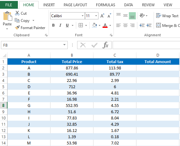
| Attendance Grades.xlsx | ||||||||||||||
|---|---|---|---|---|---|---|---|---|---|---|---|---|---|---|
|
|
||||||||||||||
| A | B | C | D | E | F | G | H | I | J | K | L | M | N | |
| 1 | Students Names | Nov 4, 2020 | Nov 3, 2020 | Nov 1, 2020 | Oct 28, 2020 | Oct 27, 2020 | Oct 21, 2020 | Oct 19, 2020 | Oct 18, 2020 | Oct 14, 2020 | Oct 13, 2020 | Oct 11, 2020 | Oct 6, 2020 | Oct 4, 2020 |
| 2 | A. D. | V | V | V | V | V | V | V | ||||||
| 3 | S. F | V | V | V | V | V | V | V | V | |||||
| 4 | S. E | V | V | V | V | V | V | V | V | V | V | |||
| 5 | A. C. | V | V | V | V | V | ||||||||
| 6 | W. E. | V | V | V | V | V | V | V | V | V | V | V | V | V |
|
Sheet2 |
Thanks
-
#4
So if I am reading this correctly you just need to count the abscence of «V»s by person?
But it also looks like you were doing something with adding a column when you were running this so is this run every day?
If you do not add a column every time the macro is run and instead prebuild the month you may be able to use just formulas.
You can use a formula like «=COUNTIF(C2:N2,»»)» at the end of every row with a person’s name and it will count up the number of absences.
If you build out the month entirely you can just add to that formula and subtract the days that have yet to pass in order to get an accurate count of the absences so far in the month.
This will save you a lot of time in adding a column every time and no VBA or macros are necessary.
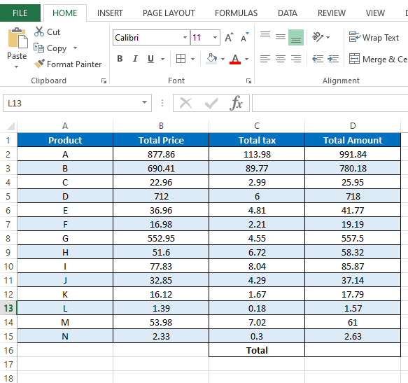
| Students Names | 4-Nov-20 | 3-Nov-20 | 1-Nov-20 | 28-Oct-20 | 27-Oct-20 | 21-Oct-20 | 19-Oct-20 | 18-Oct-20 | 14-Oct-20 | 13-Oct-20 | 11-Oct-20 | 6-Oct-20 | 4-Oct-20 | Total Absences |
| 2 | A. D. | V | V | V | V | V | V | V | 5 | |||||
| 3 | S. F | V | V | V | V | V | V | V | 5 | |||||
| 4 | S. E | V | V | V | V | V | V | V | V | V | V | 2 | ||
| 5 | A. C. | V | V | V | V | V | 7 | |||||||
| 6 | W. E. | V | V | V | V | V | V | V | V | V | V | V | V | 0 |
-
#5
Also if you wanted to go super simple you could use this in a pivot table and pull that data out very easily as well.
You would even get extra functionality like being able to filter by month or date etc.
-
#6
So if I am reading this correctly you just need to count the abscence of «V»s by person?
But it also looks like you were doing something with adding a column when you were running this so is this run every day?
If you do not add a column every time the macro is run and instead prebuild the month you may be able to use just formulas.
You can use a formula like «=COUNTIF(C2:N2,»»)» at the end of every row with a person’s name and it will count up the number of absences.
If you build out the month entirely you can just add to that formula and subtract the days that have yet to pass in order to get an accurate count of the absences so far in the month.
This will save you a lot of time in adding a column every time and no VBA or macros are necessary.
Students Names 4-Nov-20 3-Nov-20 1-Nov-20 28-Oct-20 27-Oct-20 21-Oct-20 19-Oct-20 18-Oct-20 14-Oct-20 13-Oct-20 11-Oct-20 6-Oct-20 4-Oct-20 Total Absences 2 A. D. V V V V V V V 5 3 S. F V V V V V V V 5 4 S. E V V V V V V V V V V 2 5 A. C. V V V V V 7 6 W. E. V V V V V V V V V V V V
I want to add this code in my excel so when i open a file (which contain the data in a table) i can perorm the macro on it and get my result.
-
#7
Also if you wanted to go super simple you could use this in a pivot table and pull that data out very easily as well.
You would even get extra functionality like being able to filter by month or date etc.
I have no expeirence in that, but i will try. Thanks a lot or your response
-
#8
Hello Serg…,
Insert this code in the module and run.
VBA Code:
Sub CountBlankCells()

    Dim varNColumns, varNRows, varNLoop As Long
    Dim varWorksheetName As String

    varWorksheetName = "Sheet1"

    varNColumns = Sheets(varWorksheetName).Cells(1, Columns.Count).End(xlToLeft).Column
    varNRows = Sheets(varWorksheetName).Cells(Rows.Count, 1).End(xlUp).Row

    If Sheets(varWorksheetName).Cells(1, varNColumns).Value = "Absecnce" Then
            Sheets(varWorksheetName).Columns(varNColumns).Delete
            Sheets(varWorksheetName).Cells(1, varNColumns).Value = "Absecnce"
    Else
            Sheets(varWorksheetName).Cells(1, varNColumns + 1).Value = "Absecnce"
    End If

    varNColumns = Sheets(varWorksheetName).Cells(1, Columns.Count).End(xlToLeft).Column

    For varNLoop = 2 To varNRows
       Sheets(varWorksheetName).Cells(varNLoop, varNColumns) = _
       Application.WorksheetFunction.CountBlank(Sheets(varWorksheetName).Range(Cells(varNLoop, 1), Cells(varNLoop, varNColumns - 1)))
    Next varNLoop

End Sub
-
#9
If you use Excel Max’s code you would want to convert the sub declaration from
to…
VBA Code:
Private Sub Workbook_Open()You will want to place this under the «ThisWorkbook» object for the workbook you want this to run when it opens.
I still believe that you can do what you want to do without VBA though how are your dates determined? In the example you gave the dates are pretty random, does the class not take place every day? It looks like your old macro was adding columns so are you looking for something that adds a the current date to the table when someone opens the file?
-
#10
Hello Serg…,
Insert this code in the module and run.VBA Code:
Sub CountBlankCells()

    Dim varNColumns, varNRows, varNLoop As Long
    Dim varWorksheetName As String

    varWorksheetName = "Sheet1"

    varNColumns = Sheets(varWorksheetName).Cells(1, Columns.Count).End(xlToLeft).Column
    varNRows = Sheets(varWorksheetName).Cells(Rows.Count, 1).End(xlUp).Row

    If Sheets(varWorksheetName).Cells(1, varNColumns).Value = "Absecnce" Then
            Sheets(varWorksheetName).Columns(varNColumns).Delete
            Sheets(varWorksheetName).Cells(1, varNColumns).Value = "Absecnce"
    Else
            Sheets(varWorksheetName).Cells(1, varNColumns + 1).Value = "Absecnce"
    End If

    varNColumns = Sheets(varWorksheetName).Cells(1, Columns.Count).End(xlToLeft).Column

    For varNLoop = 2 To varNRows
       Sheets(varWorksheetName).Cells(varNLoop, varNColumns) = _
       Application.WorksheetFunction.CountBlank(Sheets(varWorksheetName).Range(Cells(varNLoop, 1), Cells(varNLoop, varNColumns - 1)))
    Next varNLoop


[QUOTE="EXCEL MAX, post: 5589182, member: 468403"]
Hello Serg...,
Insert this code in the module and run.

[CODE=vba]
Sub CountBlankCells()

    Dim varNColumns, varNRows, varNLoop As Long
    Dim varWorksheetName As String

    varWorksheetName = "Sheet1"

    varNColumns = Sheets(varWorksheetName).Cells(1, Columns.Count).End(xlToLeft).Column
    varNRows = Sheets(varWorksheetName).Cells(Rows.Count, 1).End(xlUp).Row

    If Sheets(varWorksheetName).Cells(1, varNColumns).Value = "Absecnce" Then
            Sheets(varWorksheetName).Columns(varNColumns).Delete
            Sheets(varWorksheetName).Cells(1, varNColumns).Value = "Absecnce"
    Else
            Sheets(varWorksheetName).Cells(1, varNColumns + 1).Value = "Absecnce"
    End If

    varNColumns = Sheets(varWorksheetName).Cells(1, Columns.Count).End(xlToLeft).Column

    For varNLoop = 2 To varNRows
       Sheets(varWorksheetName).Cells(varNLoop, varNColumns) = _
       Application.WorksheetFunction.CountBlank(Sheets(varWorksheetName).Range(Cells(varNLoop, 1), Cells(varNLoop, varNColumns - 1)))
    Next varNLoop

End Sub
[/QUOTE]
Hello Serg…,
Insert this code in the module and run.VBA Code:
Sub CountBlankCells()

    Dim varNColumns, varNRows, varNLoop As Long
    Dim varWorksheetName As String

    varWorksheetName = "Sheet1"

    varNColumns = Sheets(varWorksheetName).Cells(1, Columns.Count).End(xlToLeft).Column
    varNRows = Sheets(varWorksheetName).Cells(Rows.Count, 1).End(xlUp).Row

    If Sheets(varWorksheetName).Cells(1, varNColumns).Value = "Absecnce" Then
            Sheets(varWorksheetName).Columns(varNColumns).Delete
            Sheets(varWorksheetName).Cells(1, varNColumns).Value = "Absecnce"
    Else
            Sheets(varWorksheetName).Cells(1, varNColumns + 1).Value = "Absecnce"
    End If

    varNColumns = Sheets(varWorksheetName).Cells(1, Columns.Count).End(xlToLeft).Column

    For varNLoop = 2 To varNRows
       Sheets(varWorksheetName).Cells(varNLoop, varNColumns) = _
       Application.WorksheetFunction.CountBlank(Sheets(varWorksheetName).Range(Cells(varNLoop, 1), Cells(varNLoop, varNColumns - 1)))
    Next varNLoop

End Sub
Thanks a lot you are very awesome, your work is very appreciated and was very helpful. I have another question,
what if i want to add another column named adjacent to the one named Absence and will be named y (Attendance Percent) Do I had to repeate the code againg? What wil be the contex of the function line? I mean: Application.WorksheetFunction. ?
And third coulmn named (Attendance Grades of 5) also.
Thanks again very much
In this lesson you can learn how to add a formula to a cell using vba. There are several ways to insert formulas to cells automatically. We can use properties like Formula, Value and FormulaR1C1 of the Range object. This post explains five different ways to add formulas to cells.
Table of contents
How to add formula to cell using VBA
Add formula to cell and fill down using VBA
Add sum formula to cell using VBA
How to add If formula to cell using VBA
Add formula to cell with quotes using VBA
Add Vlookup formula to cell using VBA
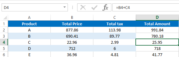
We use formulas to calculate various things in Excel. Sometimes you may need to enter the same formula to hundreds or thousands of rows or columns only changing the row numbers or columns. For an example let’s consider this sample Excel sheet.
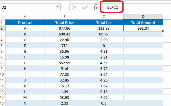
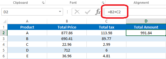
In this Excel sheet I have added a very simple formula to the D2 cell.
=B2+C2
So what if we want to add similar formulas for all the rows in column D. So the D3 cell will have the formula as =B3+C3 and D4 will have the formula as =B4+D4 and so on. Luckily we don’t need to type the formulas manually in all rows. There is a much easier way to do this. First select the cell containing the formula. Then take the cursor to the bottom right corner of the cell. Mouse pointer will change to a + sign. Then left click and drag the mouse until the end of the rows.
However if you want to add the same formula again and again for lots of Excel sheets then you can use a VBA macro to speed up the process. First let’s look at how to add a formula to one cell using vba.
How to add formula to cell using VBA
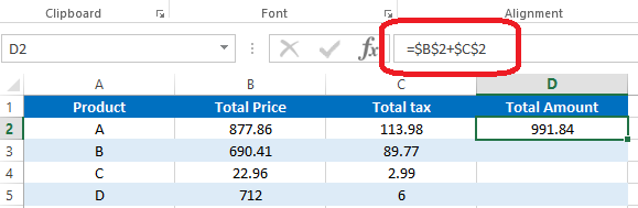
Lets see how we can enter above simple formula(=B2+C2) to cell D2 using VBA
In this method we are going to use the Formula property of the Range object.
Sub AddFormula_Method1()
Dim WS As Worksheet
Set WS = Worksheets(«Sheet1»)
WS.Range(«D2»).Formula = «=B2+C2»
End Sub
We can also use the Value property of the Range object to add a formula to a cell.
Sub AddFormula_Method2()
Dim WS As Worksheet
Set WS = Worksheets(«Sheet1»)
WS.Range(«D2»).Value = «=B2+C2»
End Sub
Next method is to use the FormulaR1C1 property of the Range object. There are few different ways to use FormulaR1C1 property. We can use absolute reference, relative reference or use both types of references inside the same formula.
In the absolute reference method cells are referred to using numbers. Excel sheets have numbers for each row. So you should think similarly for columns. So column A is number 1. Column B is number 2 etc. Then when writing the formula use R before the row number and C before the column number. So the cell A1 is referred to by R1C1. A2 is referred to by R2C1. B3 is referred to by R3C2 etc.
This is how you can use the absolute reference.
Sub AddFormula_Method3A()
Dim WS As Worksheet
Set WS = Worksheets(«Sheet1»)
WS.Range(«D2»).FormulaR1C1 = «=R2C2+R2C3»
End Sub
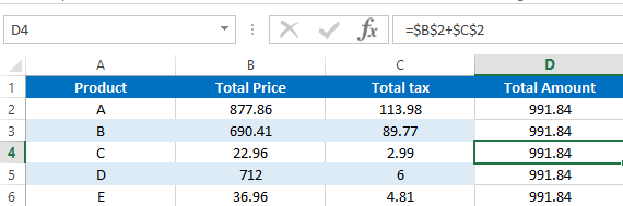
If you use the absolute reference, the formula will be added like this.
If you use the manual drag method explained above to fill down other rows, then the same formula will be copied to all the rows.
In Majority cases this is not how you want to fill down the formula. However this won’t happen in the relative method. In the relative method, cells are given numbers relative to the cell where the formula is entered. You should use negative numbers when referring to the cells in upward direction or left. Also the numbers should be placed within the square brackets. And you can omit [0] when referring to cells on the same row or column. So you can use RC[-2] instead of R[0]C[-2]. The macro recorder also generates relative reference type code, if you enter a formula to a cell while enabling the macro recorder.
Below example shows how to put formula =B2+C2 in D2 cell using relative reference method.
Sub AddFormula_Method3B()
Dim WS As Worksheet
Set WS = Worksheets(«Sheet1»)
WS.Range(«D2»).FormulaR1C1 = «=RC[-2]+RC[-1]»
End Sub
Now use the drag method to fill down all the rows.
You can see that the formulas are changed according to the row numbers.
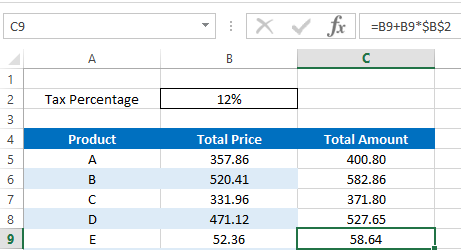
Also you can use both relative and absolute references in the same formula. Here is a typical example where you need a formula with both reference types.
We can add the formula to calculate Total Amount like this.
Sub AddFormula_Method3C()
Dim WS As Worksheet
Set WS = Worksheets(«Sheet2»)
WS.Range(«C5»).FormulaR1C1 = «=RC[-1]+RC[-1]*R2C2»
End Sub
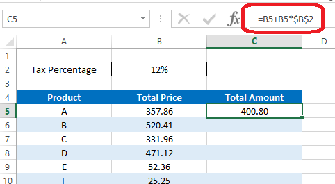
In this formula we have a absolute reference after the * symbol. So when we fill down the formula using the drag method that part will remain the same for all the rows. Hence we will get correct results for all the rows.
Add formula to cell and fill down using VBA
So now you’ve learnt various methods to add a formula to a cell. Next let’s look at how to fill down the other rows with the added formula using VBA.
Assume we have to calculate cell D2 value using =B2+C2 formula and fill down up to 1000 rows. First let’s see how we can modify the first method to do this. Let’s name this subroutine as “AddFormula_Method1_1000Rows”
Sub AddFormula_Method1_1000Rows()
End Sub
Then we need an additional variable for the For Next statement
Dim WS As Worksheet
Dim i As Integer
Next, assign the worksheet to WS variable
Set WS = Worksheets(«Sheet1»)
Now we can add the For Next statement like this.
For i = 2 To 1000
WS.Range(«D» & i).Formula = «=B» & i & «+C» & i
Next i
Here I have used «D» & i instead of D2 and «=B» & i & «+C» & i instead of «=B2+C2». So the formula keeps changing like =B3+C3, =B4+C4, =B5+C5 etc. when iterated through the For Next loop.
Below is the full code of the subroutine.
Sub AddFormula_Method1_1000Rows()
Dim WS As Worksheet
Dim i As Integer
Set WS = Worksheets(«Sheet1»)
For i = 2 To 1000
WS.Range(«D» & i).Formula = «=B» & i & «+C» & i
Next i
End Sub
So that’s how you can use VBA to add formulas to cells with variables.
Next example shows how to modify the absolute reference type of FormulaR1C1 method to add formulas upto 1000 rows.
Sub AddFormula_Method3A_1000Rows()
Dim WS As Worksheet
Dim i As Integer
Set WS = Worksheets(«Sheet1»)
For i = 2 To 1000
WS.Range(«D» & i).FormulaR1C1 = «=R» & i & «C2+R» & i & «C3»
Next i
End Sub
You don’t need to do any change to the formula section when modifying the relative reference type of the FormulaR1C1 method.
Sub AddFormula_Method3B_1000Rows()
Dim WS As Worksheet
Dim i As Integer
Set WS = Worksheets(«Sheet1»)
For i = 2 To 1000
WS.Range(«D» & i).FormulaR1C1 = «=RC[-2]+RC[-1]»
Next i
End Sub
Use similar techniques to modify other two types of subroutines to add formulas for multiple rows. Now you know how to add formulas to cells with a variable. Next let’s look at how to add formulas with some inbuilt functions using VBA.
How to add sum formula to a cell using VBA
Suppose we want the total of column D in the D16 cell. So this is the formula we need to create.
=SUM(D2:D15)
Now let’s see how to add this using VBA. Let’s name this subroutine as SumFormula.
First let’s declare a few variables.
Dim WS As Worksheet
Dim StartingRow As Long
Dim EndingRow As Long
Assign the worksheet to the variable.
Set WS = Worksheets(«Sheet3»)
Assign the starting row and the ending row to relevant variables.
StartingRow = 2
EndingRow = 1
Then the final step is to create the formula with the above variables.
WS.Range(«D16»).Formula = «=SUM(D» & StartingRow & «:D» & EndingRow & «)»
Below is the full code to add the Sum formula using VBA.
Sub SumFormula()
Dim WS As Worksheet
Dim StartingRow As Long
Dim EndingRow As Long
Set WS = Worksheets(«Sheet3»)
StartingRow = 2
EndingRow = 15
WS.Range(«D16»).Formula = «=SUM(D» & StartingRow & «:D» & EndingRow & «)»
End Sub
How to add If Formula to a cell using VBA
If function is a very popular inbuilt worksheet function available in Microsoft Excel. This function has 3 arguments. Two of them are optional.
Now let’s see how to add a If formula to a cell using VBA. Here is a typical example where we need a simple If function.
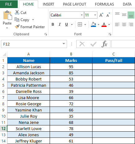
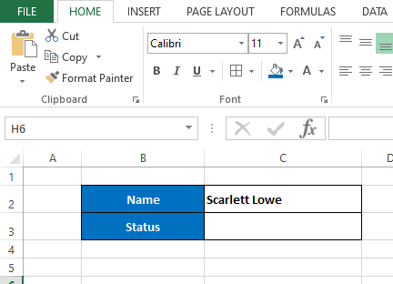
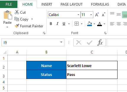
This is the results of students on an examination. Here we have names of students in column A and their marks in column B. Students should get “Pass” if he/she has marks equal or higher than 40. If marks are less than 40 then Excel should show the “Fail” in column C. We can simply obtain this result by adding an If function to column C. Below is the function we need in the C2 cell.
=IF(B2>=40,»Pass»,»Fail»)
Now let’s look at how to add this If Formula to a C2 cell using VBA. Once you know how to add it then you can use the For Next statement to fill the rest of the rows like we did above. We discussed a few different ways to add formulas to a range object using VBA. For this particular example I’m going to use the Formula property of the Range object.
So now let’s see how we can develop this macro. Let’s name this subroutine as “AddIfFormula”
Sub AddIfFormula()
End Sub
However we can’t simply add this If formula using the Formula property like we did before. Because this If formula has quotes inside it. So if we try to add the formula to the cell with quotes, then we get a syntax error.
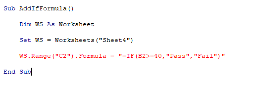
Add formula to cell with quotes
There are two ways to add the formula to a cell with quotes.
Sub AddIfFormula_Method1()
Dim WS As Worksheet
Set WS = Worksheets(«Sheet4»)
WS.Range(«C2»).Formula = «=IF(B2>=40,»»Pass»»,»»Fail»»)»
End Sub
Sub AddIfFormula_Method2()
Dim WS As Worksheet
Set WS = Worksheets(«Sheet4»)
WS.Range(«C2»).Formula = «=IF(B2>=40,» & Chr(34) & «Pass» & Chr(34) & «,» & Chr(34) & «Fail» & Chr(34) & «)»
End Sub
Add vlookup formula to cell using VBA
Finally I will show you how to add a vlookup formula to a cell using VBA. So I created a very simple example where we can use a Vlookup function. Assume we have this section in the Sheet5 of the same workbook.
So here when we change the name of the student in the C2 cell, his/her pass or fail status should automatically be shown in the C3 cell. If the original data(data we used in the above “If formula” example) is listed in the Sheet4 then we can write a Vlookup formula for the C3 cell like this.
=VLOOKUP(Sheet5!C2,Sheet4!A2:C200,3,FALSE)
We can use the Formula property of the Range object to add this Vlookup formula to the C3 using VBA.
Sub AddVlookupFormula()
Dim WS As Worksheet
Set WS = Worksheets(«Sheet5»)
WS.Range(«C3»).Formula = «=VLOOKUP(Sheet5!C2,Sheet4!A2:C200,3,FALSE)»
End Sub
With VBA, you can create a custom Function (also called a User Defined Function) that can be used in the worksheets just like regular functions.
These are helpful when the existing Excel functions are not enough. In such cases, you can create your own custom User Defined Function (UDF) to cater to your specific needs.
In this tutorial, I’ll cover everything about creating and using custom functions in VBA.
If you’re interested in learning VBA the easy way, check out my Online Excel VBA Training.
What is a Function Procedure in VBA?
A Function procedure is a VBA code that performs calculations and returns a value (or an array of values).
Using a Function procedure, you can create a function that you can use in the worksheet (just like any regular Excel function such as SUM or VLOOKUP).
When you have created a Function procedure using VBA, you can use it in three ways:
- As a formula in the worksheet, where it can take arguments as inputs and returns a value or an array of values.
- As a part of your VBA subroutine code or another Function code.
- In Conditional Formatting.
While there are already 450+ inbuilt Excel functions available in the worksheet, you may need a custom function if:
- The inbuilt functions can’t do what you want to get done. In this case, you can create a custom function based on your requirements.
- The inbuilt functions can get the work done but the formula is long and complicated. In this case, you can create a custom function that is easy to read and use.
Note that custom functions created using VBA can be significantly slower than the inbuilt functions. Hence, these are best suited for situations where you can’t get the result using the inbuilt functions.
Function Vs. Subroutine in VBA
A ‘Subroutine’ allows you to execute a set of code while a ‘Function’ returns a value (or an array of values).
To give you an example, if you have a list of numbers (both positive and negative), and you want to identify the negative numbers, here is what you can do with a function and a subroutine.
A subroutine can loop through each cell in the range and can highlight all the cells that have a negative value in it. In this case, the subroutine ends up changing the properties of the range object (by changing the color of the cells).
With a custom function, you can use it in a separate column and it can return a TRUE if the value in a cell is negative and FALSE if it’s positive. With a function, you can not change the object’s properties. This means that you can not change the color of the cell with a function itself (however, you can do it using conditional formatting with the custom function).
When you create a User Defined Function (UDF) using VBA, you can use that function in the worksheet just like any other function. I will cover more on this in the ‘Different Ways of Using a User Defined Function in Excel’ section.
Creating a Simple User Defined Function in VBA
Let me create a simple user-defined function in VBA and show you how it works.
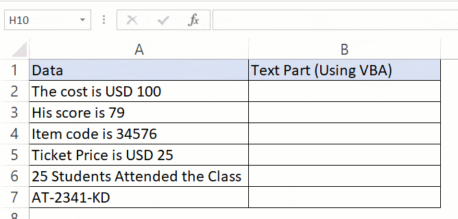
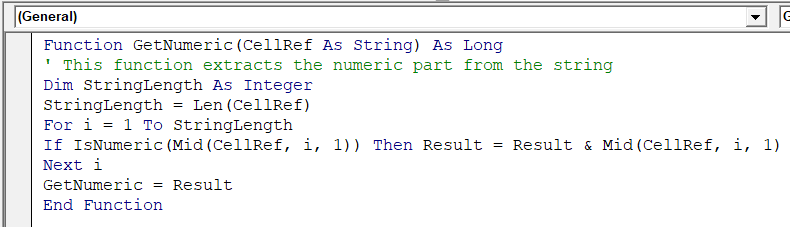
The below code creates a function that will extract the numeric parts from an alphanumeric string.
Function GetNumeric(CellRef As String) as Long
Dim StringLength As Integer
StringLength = Len(CellRef)
For i = 1 To StringLength
If IsNumeric(Mid(CellRef, i, 1)) Then Result = Result & Mid(CellRef, i, 1)
Next i
GetNumeric = Result
End Function
When you have the above code in the module, you can use this function in the workbook.
Below is how this function – GetNumeric – can be used in Excel.
Now before I tell you how this function is created in VBA and how it works, there are a few things you should know:
- When you create a function in VBA, it becomes available in the entire workbook just like any other regular function.
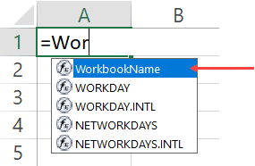
- When you type the function name followed by the equal to sign, Excel will show you the name of the function in the list of matching functions. In the above example, when I entered =Get, Excel showed me a list that had my custom function.
I believe this is a good example when you can use VBA to create a simple-to-use function in Excel. You can do the same thing with a formula as well (as shown in this tutorial), but that becomes complicated and hard to understand. With this UDF, you only need to pass one argument and you get the result.
Anatomy of a User Defined Function in VBA
In the above section, I gave you the code and showed you how the UDF function works in a worksheet.
Now let’s deep dive and see how this function is created. You need to place the below code in a module in the VB Editor. I cover this topic in the section – ‘Where to put the VBA Code for a User-Defined Function’.
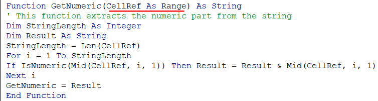
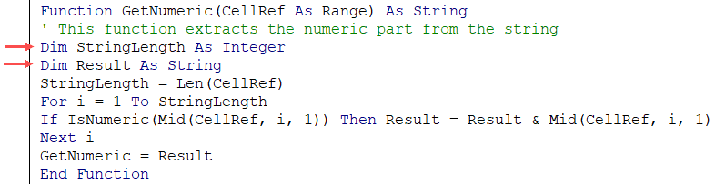
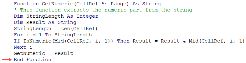
Function GetNumeric(CellRef As String) as Long
' This function extracts the numeric part from the string
Dim StringLength As Integer
StringLength = Len(CellRef)
For i = 1 To StringLength
If IsNumeric(Mid(CellRef, i, 1)) Then Result = Result & Mid(CellRef, i, 1)
Next i
GetNumeric = Result
End Function
The first line of the code starts with the word – Function.
This word tells VBA that our code is a function (and not a subroutine). The word Function is followed by the name of the function – GetNumeric. This is the name that we will be using in the worksheet to use this function.
- The name of the function cannot have spaces in it. Also, you can’t name a function if it clashes with the name of a cell reference. For example, you can not name the function ABC123 as it also refers to a cell in Excel worksheet.
- You shouldn’t give your function the same name as that of an existing function. If you do this, Excel would give preference to the in-built function.
- You can use an underscore if you want to separate words. For example, Get_Numeric is an acceptable name.
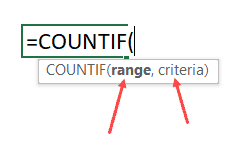
The function name is followed by some arguments in parenthesis. These are the arguments that our function would need from the user. These are just like the arguments that we need to supply to Excel’s inbuilt functions. For example in a COUNTIF function, there are two arguments (range and criteria)
Within the parenthesis, you need to specify the arguments.
In our example, there is only one argument – CellRef.
It’s also a good practice to specify what kind of argument the function expects. In this example, since we will be feeding the function a cell reference, we can specify the argument as a ‘Range’ type. If you don’t specify a data type, VBA would consider it to be a variant (which means you can use any data type).
If you have more than one arguments, you can specify those in the same parenthesis – separated by a comma. We will see later in this tutorial on how to use multiple arguments in a user-defined function.
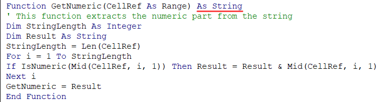
Note that the function is specified as the ‘String’ data type. This would tell VBA that the result of the formula would be of the String data type.
While I can use a numeric data type here (such as Long or Double), doing that would limit the range of numbers it can return. If I have a 20 number long string that I need to extract from the overall string, declaring the function as a Long or Double would give an error (as the number would be out of its range). Hence I have kept the function output data type as String.
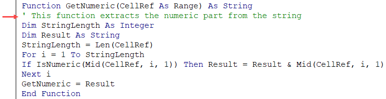
The second line of the code – the one in green that starts with an apostrophe – is a comment. When reading the code, VBA ignores this line. You can use this to add a description or a detail about the code.
The third line of the code declares a variable ‘StringLength’ as an Integer data type. This is the variable where we store the value of the length of the string that is being analyzed by the formula.
The fourth line declares the variable Result as a String data type. This is the variable where we will extract the numbers from the alphanumeric string.
The fifth line assigns the length of the string in the input argument to the ‘StringLength’ variable. Note that ‘CellRef’ refers to the argument that will be given by the user while using the formula in the worksheet (or using it in VBA – which we will see later in this tutorial).
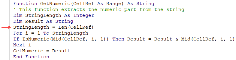
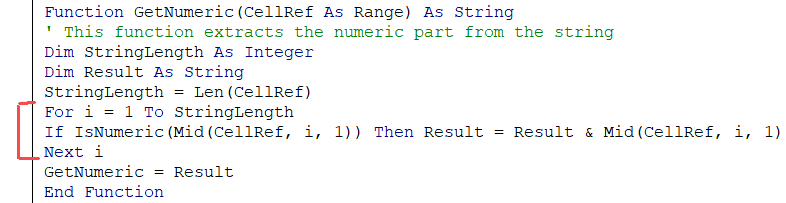
Sixth, seventh, and eighth lines are the part of the For Next loop. The loop runs for as many times as many characters are there in the input argument. This number is given by the LEN function and is assigned to the ‘StringLength’ variable.
So the loop runs from ‘1 to Stringlength’.
Within the loop, the IF statement analyzes each character of the string and if it’s numeric, it adds that numeric character to the Result variable. It uses the MID function in VBA to do this.
The second last line of the code assigns the value of the result to the function. It’s this line of code that ensures that the function returns the ‘Result’ value back in the cell (from where it’s called).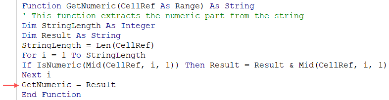
The last line of the code is End Function. This is a mandatory line of code that tells VBA that the function code ends here.
The above code explains the different parts of a typical custom function created in VBA. In the following sections, we will deep dive into these elements and also see the different ways to execute the VBA function in Excel.
Arguments in a User Defined Function in VBA
In the above examples, where we created a user-defined function to get the numeric part from an alphanumeric string (GetNumeric), the function was designed to take one single argument.
In this section, I will cover how to create functions that take no argument to the ones that take multiple arguments (required as well as optional arguments).
Creating a Function in VBA without Any Arguments
In Excel worksheet, we have several functions that take no arguments (such as RAND, TODAY, NOW).
These functions are not dependent on any input arguments. For example, the TODAY function would return the current date and the RAND function would return a random number between 0 and 1.
You can create such similar function in VBA as well.
Below is the code that will give you the name of the file. It doesn’t take any arguments as the result it needs to return is not dependent on any argument.
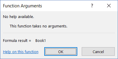
Function WorkbookName() As String
WorkbookName = ThisWorkbook.Name
End Function
The above code specifies the function’s result as a String data type (as the result we want is the file name – which is a string).
This function assigns the value of ‘ThisWorkbook.Name’ to the function, which is returned when the function is used in the worksheet.
If the file has been saved, it returns the name with the file extension, else it simply gives the name.
The above has one issue though.
If the file name changes, it wouldn’t automatically update. Normally a function refreshes whenever there is a change in the input arguments. But since there are no arguments in this function, the function doesn’t recalculate (even if you change the name of the workbook, close it and then reopen again).
If you want, you can force a recalculation by using the keyboard shortcut – Control + Alt + F9.
To make the formula recalculate whenever there is a change in the worksheet, you need to a line of code to it.
The below code makes the function recalculate whenever there is a change in the worksheet (just like other similar worksheet functions such as TODAY or RAND function).
Function WorkbookName() As String
Application.Volatile True
WorkbookName = ThisWorkbook.Name
End Function
Now, if you change the workbook name, this function would update whenever there is any change in the worksheet or when you reopen this workbook.
Creating a Function in VBA with One Argument
In one of the sections above, we have already seen how to create a function that takes only one argument (the GetNumeric function covered above).
Let’s create another simple function that takes only one argument.
Function created with the below code would convert the referenced text into uppercase. Now we already have a function for it in Excel, and this function is just to show you how it works. If you have to do this, it’s better to use the inbuilt UPPER function.
Function ConvertToUpperCase(CellRef As Range)
ConvertToUpperCase = UCase(CellRef)
End Function
This function uses the UCase function in VBA to change the value of the CellRef variable. It then assigns the value to the function ConvertToUpperCase.
Since this function takes an argument, we don’t need to use the Application.Volatile part here. As soon as the argument changes, the function would automatically update.
Creating a Function in VBA with Multiple Arguments
Just like worksheet functions, you can create functions in VBA that takes multiple arguments.
The below code would create a function that will extract the text before the specified delimiter. It takes two arguments – the cell reference that has the text string, and the delimiter.
Function GetDataBeforeDelimiter(CellRef As Range, Delim As String) as String
Dim Result As String
Dim DelimPosition As Integer
DelimPosition = InStr(1, CellRef, Delim, vbBinaryCompare) - 1
Result = Left(CellRef, DelimPosition)
GetDataBeforeDelimiter = Result
End Function
When you need to use more than one argument in a user-defined function, you can have all the arguments in the parenthesis, separated by a comma.
Note that for each argument, you can specify a data type. In the above example, ‘CellRef’ has been declared as a range datatype and ‘Delim’ has been declared as a String data type. If you don’t specify any data type, VBA considers these are a variant data type.
When you use the above function in the worksheet, you need to give the cell reference that has the text as the first argument and the delimiter character(s) in double quotes as the second argument.
It then checks for the position of the delimiter using the INSTR function in VBA. This position is then used to extract all the characters before the delimiter (using the LEFT function).
Finally, it assigns the result to the function.
This formula is far from perfect. For example, if you enter a delimiter that is not found in the text, it would give an error. Now you can use the IFERROR function in the worksheet to get rid of the errors, or you can use the below code that returns the entire text when it can’t find the delimiter.
Function GetDataBeforeDelimiter(CellRef As Range, Delim As String) as String
Dim Result As String
Dim DelimPosition As Integer
DelimPosition = InStr(1, CellRef, Delim, vbBinaryCompare) - 1
If DelimPosition < 0 Then DelimPosition = Len(CellRef)
Result = Left(CellRef, DelimPosition)
GetDataBeforeDelimiter = Result
End Function
We can further optimize this function.
If you enter the text (from which you want to extract the part before the delimiter) directly in the function, it would give you an error. Go ahead.. try it!
This happens as we have specified the ‘CellRef’ as a range data type.
Or, if you want the delimiter to be in a cell and use the cell reference instead of hard coding it in the formula, you can’t do that with the above code. It’s because the Delim has been declared as a string datatype.
If you want the function to have the flexibility to accept direct text input or cell references from the user, you need to remove the data type declaration. This would end up making the argument as a variant data type, which can take any type of argument and process it.
The below code would do this:
Function GetDataBeforeDelimiter(CellRef, Delim) As String
Dim Result As String
Dim DelimPosition As Integer
DelimPosition = InStr(1, CellRef, Delim, vbBinaryCompare) - 1
If DelimPosition < 0 Then DelimPosition = Len(CellRef)
Result = Left(CellRef, DelimPosition)
GetDataBeforeDelimiter = Result
End Function
Creating a Function in VBA with Optional Arguments
There are many functions in Excel where some of the arguments are optional.
For example, the legendary VLOOKUP function has 3 mandatory arguments and one optional argument.
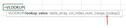
An optional argument, as the name suggests, is optional to specify. If you don’t specify one of the mandatory arguments, your function is going to give you an error, but if you don’t specify the optional argument, your function would work.
But optional arguments are not useless. They allow you to choose from a range of options.
For example, in the VLOOKUP function, if you don’t specify the fourth argument, VLOOKUP does an approximate lookup and if you specify the last argument as FALSE (or 0), then it does an exact match.
Remember that the optional arguments must always come after all the required arguments. You can’t have optional arguments at the beginning.
Now let’s see how to create a function in VBA with optional arguments.
Function with Only an Optional Argument
As far as I know, there is no inbuilt function that takes optional arguments only (I can be wrong here, but I can’t think of any such function).
But we can create one with VBA.
Below is the code of the function that will give you the current date in the dd-mm-yyyy format if you don’t enter any argument (i.e. leave it blank), and in “dd mmmm, yyyy” format if you enter anything as the argument (i.e., anything so that the argument is not blank).
Function CurrDate(Optional fmt As Variant)
Dim Result
If IsMissing(fmt) Then
CurrDate = Format(Date, "dd-mm-yyyy")
Else
CurrDate = Format(Date, "dd mmmm, yyyy")
End If
End Function
Note that the above function uses ‘IsMissing’ to check whether the argument is missing or not. To use the IsMissing function, your optional argument must be of the variant data type.
The above function works no matter what you enter as the argument. In the code, we only check if the optional argument is supplied or not.
You can make this more robust by taking only specific values as arguments and showing an error in rest of the cases (as shown in the below code).
Function CurrDate(Optional fmt As Variant)
Dim Result
If IsMissing(fmt) Then
CurrDate = Format(Date, "dd-mm-yyyy")
ElseIf fmt = 1 Then
CurrDate = Format(Date, "dd mmmm, yyyy")
Else
CurrDate = CVErr(xlErrValue)
End If
End Function
The above code creates a function that shows the date in the “dd-mm-yyyy” format if no argument is supplied, and in “dd mmmm,yyyy” format when the argument is 1. It gives an error in all other cases.
Function with Required as well as Optional Arguments
We have already seen a code that extracts the numeric part from a string.
Now let’s have a look at a similar example that takes both required as well as optional arguments.
The below code creates a function that extracts the text part from a string. If the optional argument is TRUE, it gives the result in uppercase, and if the optional argument is FALSE or is omitted, it gives the result as is.
Function GetText(CellRef As Range, Optional TextCase = False) As String
Dim StringLength As Integer
Dim Result As String
StringLength = Len(CellRef)
For i = 1 To StringLength
If Not (IsNumeric(Mid(CellRef, i, 1))) Then Result = Result & Mid(CellRef, i, 1)
Next i
If TextCase = True Then Result = UCase(Result)
GetText = Result
End Function
Note that in the above code, we have initialized the value of ‘TextCase’ as False (look within the parenthesis in the first line).
By doing this, we have ensured that the optional argument starts with the default value, which is FALSE. If the user specifies the value as TRUE, the function returns the text in upper case, and if the user specifies the optional argument as FALSE or omits it, then the text returned is as is.
Creating a Function in VBA with an Array as the Argument
So far we have seen examples of creating a function with Optional/Required arguments – where these arguments were a single value.
You can also create a function that can take an array as the argument. In Excel worksheet functions, there are many functions that take array arguments, such as SUM, VLOOKUP, SUMIF, COUNTIF, etc.
Below is the code that creates a function that gives the sum of all the even numbers in the specified range of the cells.
Function AddEven(CellRef as Range)
 Dim Cell As Range
 For Each Cell In CellRef
 If IsNumeric(Cell.Value) Then
 If Cell.Value Mod 2 = 0 Then
 Result = Result + Cell.Value
 End If
 End If
 Next Cell
 AddEven = Result
 End Function
You can use this function in the worksheet and provide the range of cells that have the numbers as the argument. The function would return a single value – the sum of all the even numbers (as shown below).
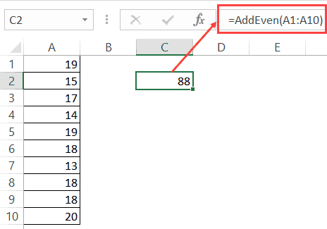
In the above function, instead of a single value, we have supplied an array (A1:A10). For this to work, you need to make sure your data type of the argument can accept an array.
In the code above, I specified the argument CellRef as Range (which can take an array as the input). You can also use the variant data type here.
In the code, there is a For Each loop that goes through each cell and checks if it’s a number of not. If it isn’t, nothing happens and it moves to the next cell. If it’s a number, it checks if it’s even or not (by using the MOD function).
In the end, all the even numbers are added and teh sum is assigned back to the function.
Creating a Function with Indefinite Number of Arguments
While creating some functions in VBA, you may not know the exact number of arguments that a user wants to supply. So the need is to create a function that can accept as many arguments are supplied and use these to return the result.
An example of such worksheet function is the SUM function. You can supply multiple arguments to it (such as this):
=SUM(A1,A2:A4,B1:B20)
The above function would add the values in all these arguments. Also, note that these can be a single cell or an array of cells.
You can create such a function in VBA by having the last argument (or it could be the only argument) as optional. Also, this optional argument should be preceded by the keyword ‘ParamArray’.
‘ParamArray’ is a modifier that allows you to accept as many arguments as you want. Note that using the word ParamArray before an argument makes the argument optional. However, you don’t need to use the word Optional here.
Now let’s create a function that can accept an arbitrary number of arguments and would add all the numbers in the specified arguments:
Function AddArguments(ParamArray arglist() As Variant)
For Each arg In arglist
AddArguments = AddArguments + arg
Next arg
End Function
The above function can take any number of arguments and add these arguments to give the result.
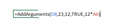
Note that you can only use a single value, a cell reference, a boolean, or an expression as the argument. You can not supply an array as the argument. For example, if one of your arguments is D8:D10, this formula would give you an error.
If you want to be able to use both multi-cell arguments you need to use the below code:
Function AddArguments(ParamArray arglist() As Variant)
For Each arg In arglist
For Each Cell In arg
AddArguments = AddArguments + Cell
Next Cell
Next arg
End Function
Note that this formula works with multiple cells and array references, however, it can not process hardcoded values or expressions. You can create a more robust function by checking and treating these conditions, but that’s not the intent here.
The intent here is to show you how ParamArray works so you can allow an indefinite number of arguments in the function. In case you want a better function than the one created by the above code, use the SUM function in the worksheet.
Creating a Function that Returns an Array
So far we have seen functions that return a single value.
With VBA, you can create a function that returns a variant that can contain an entire array of values.
Array formulas are also available as inbuilt functions in Excel worksheets. If you’re familiar with array formulas in Excel, you would know that these are entered using Control + Shift + Enter (instead of just the Enter). You can read more about array formulas here. If you don’t know about array formulas, don’t worry, keep reading.
Let’s create a formula that returns an array of three numbers (1,2,3).
The below code would do this.
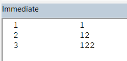
Function ThreeNumbers() As Variant
Dim NumberValue(1 To 3)
NumberValue(1) = 1
NumberValue(2) = 2
NumberValue(3) = 3
ThreeNumbers = NumberValue
End Function
In the above code, we have specified the ‘ThreeNumbers’ function as a variant. This allows it to hold an array of values.
The variable ‘NumberValue’ is declared as an array with 3 elements. It holds the three values and assigns it to the ‘ThreeNumbers’ function.
You can use this function in the worksheet by entering the function and hitting the Control + Shift + Enter key (hold the Control and the Shift keys and then press Enter).
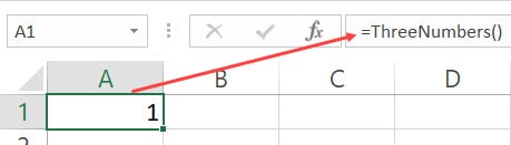
When you do this, it will return 1 in the cell, but in reality, it holds all the three values. To check this, use the below formula:
=MAX(ThreeNumbers())
Use the above function with Control + Shift + Enter. You will notice that the result is now 3, as it is the largest values in the array returned by the Max function, which gets the three numbers as the result of our user-defined function – ThreeNumbers.
You can use the same technique to create a function that returns an array of Month Names as shown by the below code:
Function Months() As Variant
Dim MonthName(1 To 12)
MonthName(1) = "January"
MonthName(2) = "February"
MonthName(3) = "March"
MonthName(4) = "April"
MonthName(5) = "May"
MonthName(6) = "June"
MonthName(7) = "July"
MonthName(8) = "August"
MonthName(9) = "September"
MonthName(10) = "October"
MonthName(11) = "November"
MonthName(12) = "December"
Months = MonthName
End Function
Now when you enter the function =Months() in Excel worksheet and use Control + Shift + Enter, it will return the entire array of month names. Note that you see only January in the cell as that is the first value in the array. This does not mean that the array is only returning one value.
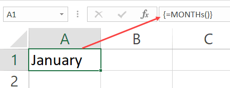
To show you the fact that it is returning all the values, do this – select the cell with the formula, go to the formula bar, select the entire formula and press F9. This will show you all the values that the function returns.

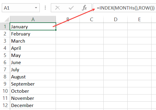
You can use this by using the below INDEX formula to get a list of all the month names in one go.
=INDEX(Months(),ROW())
Now if you have a lot of values, it’s not a good practice to assign these values one by one (as we have done above). Instead, you can use the Array function in VBA.
So the same code where we create the ‘Months’ function would become shorter as shown below:
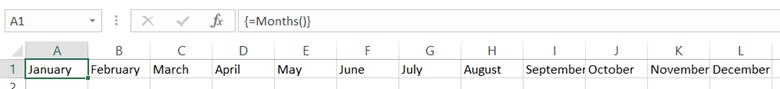
Function Months() As Variant
Months = Array("January", "February", "March", "April", "May", "June", _
"July", "August", "September", "October", "November", "December")
End Function
The above function uses the Array function to assign the values directly to the function.
Note that all the functions created above return a horizontal array of values. This means that if you select 12 horizontal cells (let’s say A1:L1), and enter the =Months() formula in cell A1, it will give you all the month names.
But what if you want these values in a vertical range of cells.
You can do this by using the TRANSPOSE formula in the worksheet.
Simply select 12 vertical cells (contiguous), and enter the below formula.
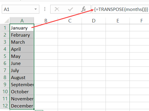
Understanding the Scope of a User Defined Function in Excel
A function can have two scopes – Public or Private.
- A Public scope means that the function is available for all the sheets in the workbook as well as all the procedures (Sub and Function) across all modules in the workbook. This is useful when you want to call a function from a subroutine (we will see how this is done in the next section).
- A Private scope means that the function is available only in the module in which it exists. You can’t use it in other modules. You also won’t see it in the list of functions in the worksheet. For example, if your Function name is ‘Months()’, and you type function in Excel (after the = sign), it will not show you the function name. You can, however, still, use it if you enter the formula name.
If you don’t specify anything, the function is a Public function by default.
Below is a function that is a Private function:
Private Function WorkbookName() As String
WorkbookName = ThisWorkbook.Name
End Function
You can use this function in the subroutines and the procedures in the same modules, but can’t use it in other modules. This function would also not show up in the worksheet.
The below code would make this function Public. It will also show up in the worksheet.
Function WorkbookName() As String
WorkbookName = ThisWorkbook.Name
End Function
Different Ways of Using a User Defined Function in Excel
Once you have created a user-defined function in VBA, you can use it in many different ways.
Let’s first cover how to use the functions in the worksheet.
Using UDFs in Worksheets
We have already seen examples of using a function created in VBA in the worksheet.
All you need to do is enter the functions name, and it shows up in the intellisense.
Note that for the function to show up in the worksheet, it must be a Public function (as explained in the section above).
You can also use the Insert Function dialog box to insert the user defined function (using the steps below). This would work only for functions that are Public.
The above steps would insert the function in the worksheet. It also displays a Function Arguments dialog box that will give you details on the arguments and the result.
You can use a user defined function just like any other function in Excel. This also means that you can use it with other inbuilt Excel functions. For example. the below formula would give the name of the workbook in upper case:
=UPPER(WorkbookName())
Using User Defined Functions in VBA Procedures and Functions
When you have created a function, you can use it in other sub-procedures as well.
If the function is Public, it can be used in any procedure in the same or different module. If it’s Private, it can only be used in the same module.
Below is a function that returns the name of the workbook.
Function WorkbookName() As String
WorkbookName = ThisWorkbook.Name
End Function
The below procedure call the function and then display the name in a message box.
Sub ShowWorkbookName()
MsgBox WorkbookName
End Sub
You can also call a function from another function.
In the below codes, the first code returns the name of the workbook, and the second one returns the name in uppercase by calling the first function.
Function WorkbookName() As String
WorkbookName = ThisWorkbook.Name
End Function
Function WorkbookNameinUpper()
WorkbookNameinUpper = UCase(WorkbookName)
End Function
Calling a User Defined Function from Other Workbooks
If you have a function in a workbook, you can call this function in other workbooks as well.
There are multiple ways to do this:
- Creating an Add-in
- Saving function in the Personal Macro Workbook
- Referencing the function from another workbook.
Creating an Add-in
By creating and installing an add-in, you will have the custom function in it available in all the workbooks.
Suppose you have created a custom function – ‘GetNumeric’ and you want it in all the workbooks. To do this, create a new workbook and have the function code in a module in this new workbook.
Now follow the steps below to save it as an add-in and then install it in Excel.
Now the add-in has been activated.
Now you can use the custom function in all the workbooks.
Saving the Function in Personal Macro Workbook
A Personal Macro Workbook is a hidden workbook in your system that opens whenever you open the Excel application.
It’s a place where you can store macro codes and then access these macros from any workbook. It’s a great place to store those macros that you want to use often.
By default, there is no personal macro workbook in your Excel. You need to create it by recording a macro and saving it in the Personal macro workbook.
You can find the detailed steps on how to create and save macros in the personal macro workbook here.
Referencing the function from another workbook
While the first two methods (creating an add-in and using personal macro workbook) would work in all situations, if you want to reference the function from another workbook, that workbook needs to be open.
Suppose you have a workbook with the name ‘Workbook with Formula’, and it has the function with the name ‘GetNumeric’.
To use this function in another workbook (while the Workbook with Formula is open), you can use the below formula:
=’Workbook with Formula’!GetNumeric(A1)
The above formula will use the user defined function in the Workbook with Formula file and give you the result.
Note that since the workbook name has spaces, you need to enclose it in single quotes.
Using Exit Function Statement VBA
If you want to exit a function while the code is running, you can do that by using the ‘Exit Function’ statement.
The below code would extract the first three numeric characters from an alphanumeric text string. As soon as it gets the three characters, the function ends and returns the result.
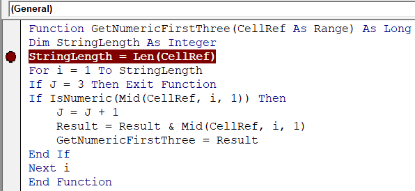
Function GetNumericFirstThree(CellRef As Range) As Long
Dim StringLength As Integer
StringLength = Len(CellRef)
For i = 1 To StringLength
If J = 3 Then Exit Function
If IsNumeric(Mid(CellRef, i, 1)) Then
J = J + 1
Result = Result & Mid(CellRef, i, 1)
GetNumericFirstThree = Result
End If
Next i
End Function
The above function checks for the number of characters that are numeric, and when it gets 3 numeric characters, it Exits the function in the next loop.
Debugging a User Defined Function
There are a few techniques you can use while debugging a user-defined function in VBA:
Debugging a Custom Function by Using the Message Box
Use MsgBox function to show a message box with a specific value.
The value you display can be based on what you want to test. For example, if you want to check if the code is getting executed or not, any message would work, and if you want to check whether the loops are working or not, you can display a specific value or the loop counter.
Debugging a Custom Function by Setting the Breakpoint
Set a breakpoint to be able to go step through each line one at a time. To set a breakpoint, select the line where you want it and press F9, or click on the gray vertical area which is left to the code lines. Any of these methods would insert a breakpoint (you will see a red dot in the gray area).
Once you have set the breakpoint and you execute the function, it goes till the breakpoint line and then stops. Now you can step through the code using the F8 key. Pressing F8 once moves to the next line in the code.
Debugging a Custom Function by Using Debug.Print in the Code
You can use Debug.Print statement in your code to get the values of the specified variables/arguments in the immediate window.
For example, in the below code, I have used Debug.Print to get the value of two variables – ‘j’ and ‘Result’
Function GetNumericFirstThree(CellRef As Range) As Long
Dim StringLength As Integer
StringLength = Len(CellRef)
For i = 1 To StringLength
If J = 3 Then Exit Function
If IsNumeric(Mid(CellRef, i, 1)) Then
 J = J + 1
 Result = Result & Mid(CellRef, i, 1)
 Debug.Print J, Result
 GetNumericFirstThree = Result
End If
Next i
End Function
When this code is executed, it shows the following in the immediate window.
Excel Inbuilt Functions Vs. VBA User Defined Function
There are few strong benefits of using Excel in-built functions over custom functions created in VBA.
- Inbuilt functions are a lot faster than the VBA functions.
- When you create a report/dashboard using VBA functions, and you send it to a client/colleague, they wouldn’t have to worry about whether the macros are enabled or not. In some cases, clients/customers get scared by seeing a warning in the yellow bar (which simply asks them to enable macros).
- With inbuilt Excel functions, you don’t need to worry about file extensions. If you have macros or user-defined functions in the workbook, you need to save it in .xlsm.
While there are many strong reasons to use Excel in-built functions, in a few cases, you’re better off using a user-defined function.
- It’s better to use a user-defined function if your inbuilt formula is huge and complicated. This becomes even more relevant when you need someone else to update the formulas. For example, if you have a huge formula made up of many different functions, even changing a reference to a cell can be tedious and error-prone. Instead, you can create a custom function that only takes one or two arguments and does all the heavy lifting the backend.
- When you have to get something done that can not be done by Excel inbuilt functions. An example of this can be when you want to extract all the numeric characters from a string. In such cases, the benefit of using a user-defined function gar outweighs its negatives.
Where to put the VBA Code for a User-Defined Function
When creating a custom function, you need to put the code in the code window for the workbook in which you want the function.
Below are the steps to put the code for the ‘GetNumeric’ function in the workbook.
- Go to the Developer tab.

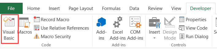
- Click on the Visual Basic option. This will open the VB editor in the backend.
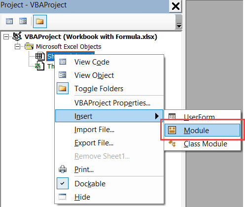
- In the Project Explorer pane in the VB Editor, right-click on any object for the workbook in which you want to insert the code. If you don’t see the Project Explorer go to the View tab and click on Project Explorer.
- Go to Insert and click on Module. This will insert a module object for your workbook.

- Copy and paste the code in the module window.

You May Also Like the Following Excel VBA Tutorials:
- Working with Cells and Ranges in Excel VBA.
- Working with Worksheets in Excel VBA.
- Working with Workbooks using VBA.
- How to use Loops in Excel VBA.
- Excel VBA Events – An Easy (and Complete) Guide
- Using IF Then Else Statements in VBA.
- How to Record a Macro in Excel.
- How to Run a Macro in Excel.
- How to Sort Data in Excel using VBA (A Step-by-Step Guide).
- Excel VBA InStr Function – Explained with Examples.
Probably one of the coolest benefits of learning VBA is the ability to create your own functions.
In Excel, there are more than 450 functions, and some of them are highly useful in your daily work. But Excel gives you the ability to create a custom function using VBA. Yes, you get it right. USER DEFINED Function, in short UDF, or you can also call it a Custom VBA function.
And there’s one thing that I can say with confidence every aspiring VBA user wants to learn to create a User Defined Function. Don’t you? Say “Yes” in the comment section, if you are one of those people who want to create a custom function.
I’m excited to tell you that this is a COMPLETE GUIDE to help you to create your first custom function using VBA and apart from this I have shared some examples of USER-DEFINED Functions to help you to get inspired.
- Here I’ll be using the words User Defined Function, custom function, and UDF interchangeably. So stay with me you are going to be a VBA rock star in the next couple of minutes.
- To create a code for the VBA custom function you need to write it, you can’t record it using the macro recorder.
Why You Should Create a Custom Excel Function
As I said, there are a lot of in-built functions in Excel which can help you to solve almost all the problems and do all kinds of calculations. But, sometimes, in specific situations, you need to create a UDF.
And, below I have listed some of the reasons or situations in which you need to go with a custom function.
1. When there is no Function for this
This is one of the common reasons for creating a UDF with VBA, because sometimes that you need to calculate something and there is no specific function for this. I can give you an example of counting words from a cell and for this, I found a UDF can be a perfect solution.

2. Replace a Complex Formula
If you work with formulas, I’m sure you know this thing that complex formulas are hard to read and sometimes harder to understand by others. So a custom function can a solution to this problem because once you create a UDF you don’t need to write that complex formula again and again.

3. When you don’t want to use SUB Routine
While you can use a VBA code to perform a calculation but VBA codes are not dynamic*. You need to run that code again if you want to update your calculation. But if you convert that code into a function then you don’t need to run that code again and again as you can simply insert it as a function.
How to Create Your First User Defined Function in Excel
OK so look. I have split the entire process into three steps:
- Declaring your Procedure as a Function
- Defining its Arguments and their Data Type
- Add code to Calculate the Desired Value
But let me give you can:
You need to create a function that can return the name of the day from a date value. Well, we have a function that returns the day number for the week but not the name. You got it what I’m saying? Yes?
So, let’s follow the below steps to create your first user-defined function:
- First of all, open your visual basic editor by using the shortcut key ALT + F11 or go to Developer Tab and simply click on the “Visual Basic” button.

- The next thing is to insert a module, so right-click on the VBA project window and then go to insert, and after that click “Module”. (ALERT: You need to enter a USER DEFINED FUNCTION only into standard modules. Sheet and ThisWorkbook modules both are a special type of module and if you enter a UDF in these two modules, Excel does not recognize that you are creating a UDF).
- The third thing is to define a name for the function and here I’m using “myDayName”. So you must write “Function mydayName”. Why Function before the Name? As you are creating a VBA function so the using the word “Function” tells Excel to treat this code as a function (make sure to read the scope of a UDF ahead in the post).
- After that, you need to define arguments for your function. So insert starting parentheses and write “InputDate As Date”. Here InputDate is the Argument’s name and date is its data type. It’s always better to define a data type for the argument.
- Now, close the parentheses and write “As String”. Here you are defining the data type of the result returns by the function and as you want day name which is a text so its data type should be as “String”. If you want to have the result which is other than a string make sure to define its data type according to that. (Function myDayName(InputDate As Date) As String).
- In the end, hit ENTER. At this point, your function’s name, its argument, argument’s data type, and function’s data type is defined and you have something like below in your module:
- Now within the “Function” and “End Function”, you need to define the calculation or you can say working of this UDF. In Excel, there is a worksheet function called “Text” and we are using the same here. And for this, you need to write the below code and with this code, you are defining the value which should be returned by the function. myDayName = WorksheetFunction.Text(InputDate, “dddddd”)
- Now, close your VB editor and go back to the worksheet and in the cell B2, enter “=myDayName(A2)” hit enter and you’ll have the day name.


Congratulations! You have just created your first User Defined Function. This is the moment of real Joy. Isn’t it? Type “Joy” in the comment section.
How this Function Works and Return Value in a Cell
Your first custom function is here, but the thing is, you need to understand how it works. If I say in simple words, it’s a VBA code but you have used it as a function procedure. Let’s divide it into three parts:
- You enter it in a Cell as Function and Specify the Input Value.
- Excel runs the code behind the function and uses the value which you have referred to.
- You got the result in the cell.
But you need to understand how this function works from inside. So I have split the entire process into three different parts where you can see how the code which you have written for the function actually works.

As you have specified “InputDate” as the argument for the function and when you enter the function in the cell and specify a date, VBA takes that date value and supply it to the text function which you have used in the code.
And in the example which I have mentioned above, the date you have in the cell A1 is 01-Jan-2019.
After that, the TEXT function converts that date into a day using the format code “dddddd” which you have already mentioned in the function code. And that day which is returns by the TEXT function is assigned to the “myDayName”.
So if the result of the TEXT function is Tuesday that value will be assigned to the “myDayName”.
And here the working of the function comes to an end. “myDayName” is the name of the function so any value is which is assigned to “myDayName” will be the result value and the function which you have inserted in the worksheet will return it in the cell.
When you write a code for a custom function there one thing you need to take care that the value which that code return must be assigned to the function’s name.
How to Improve a UDF for Good
Well, you know how to create a custom VBA function.
Now…
There’s one thing you need to take care that the code you have used to function should be good enough to handle all the possibilities. If you talk about the function which you just wrote above can return the day name from a date.
But…
What if the value you have specified will not a date? And if the cell you have referred is blank? There can be other possibilities but I’m sure you got my point.
Right? So, let’s try to improve this custom function which could be able to deal with the above problems. Alright. First of all, you need to change the data type of the argument and use:
InputDate As VariantWith this, your custom function can take any kind of data type as input. Next, we need to use VBA IF statement to check InputDate for some conditions. The first condition is if the cell is blank or not. And for this, you need to use below code:
If InputDate = "" Then
myDayName = ""
This will make the function return blank if the cell you have referred is blank.
One problem is solved, let’s get into the next one. Other than a date there are possibilities that you can have a number or a text. So, for this, you also need to create a condition which should check whether the value referred is an actual date or not.
The code would be:
If IsDate(InputDate) = False Then
myDateName = ""
Here I’m using a blank for both of the conditions, so that if you have large data, you could easily filter values where the input value is not valid. So, after adding the above conditions, the code would look like:
Function myDayName(InputDate As Variant) As String
If InputDate = "" Then
myDayName = ""
Else
If IsDate(InputDate) = False Then
myDateName = ""
Else
myDayName = WorksheetFunction.Text(InputDate, "dddddd")
End If
End If
End Function
And here’s how it works now: I’m sure you can still make some changes in this function but I’m sure you got my point clearly.
How to use a Custom VBA Function
At this point, you’re pretty much clear about how you can create a VBA function in Excel. But once you have it, you need to know how you can use it. And in this part of the post, I’m going to share with you how and where you can use it. So, let’s jump into it.
1. Simply within a Worksheet
Why we create a custom function? Simple. To use it in the worksheet. You can simply enter a UDF in a worksheet by using equal sign and type name of the function and then specify it’s arguments.

You can also enter a user defined function from the function library. Go to Formula Tab ➜ Insert Function ➜ User Defined.

From this list, you can choose the UDF you want to insert.
2. Using in other Sub Procedures and Functions
You can also use a function within other functions or in a “Sub” procedure. Below is a VBA code where you have used the function to get day name for the current date.
Sub todayDay()
MsgBox "Today is " & myDayName(Date)
End Sub
Make sure to read “Scope of a UDF” ahead in this post to learn more on using a function in other procedures.
3. Accessing Functions from Other Workbook
If you have a UDF in one workbook and you want to use it in another workbook or in all the workbooks, you do it by making an add-in for it. Follow these simple steps:
- First of all, to you need to save the file (in which you have the custom function code) as an add-in.
- For this, go to the File Tab ➜ Save As ➜ “Excel Add-Ins (.xalm).

- After that, double-click on the add-in you and install it.

That’s it. Now you can use all of your VBA functions in any of the workbook.
Different Ways to Create a Custom VBA Function [Advanced Level]
At this point, you know about to create a custom function in VBA. But the thing is when we use In-Built functions, they come with different type of arguments.
So in this section of this guide, you gonna learn how to create a UDF with the different type of arguments.
- Without Any Arguments
- With Just One Argument
- With Multiple Arguments
- Using Array as the Argument
…let’s move ahead.
1. Without Any Arguments
Do you remember about functions like NOW and TODAY where you don’t need to enter any argument?
Yes. You can create a User Defined Function where you don’t need to enter an argument. Let’s do it with an example:
Let’s create a custom function which can return the location of the current file. And here’s the code:
Function myPath() As String
Dim myLocation As String
Dim myName As String
myLocation = ActiveWorkbook.FullName
myName = ActiveWorkbook.Name
If myLocation = myName Then
myPath = "File is not saved yet."
Else
myPath = myLocation
End If
End Function
This function returns the path of the location where the current file is stored and if the workbook is not stored anywhere, it will show a message says “File is not saved yet”.

Now, if you pay close attention to the code of this function, you don’t have defined any argument (within the bracket). You have just defined the data type for the function’s result.
The basic rule of creating a function without argument is a code where you don’t need to input anything.
In simple words, the value you want to have in return from the function should be calculated automatically.
And in this function, you have the same thing.
This code ActiveWorkbook.FullName returns the location of the file and this one ActiveWorkbook.Name returns the name. You don’t need to input anything.
2. With Just One Argument
We have already covered this thing while learning how to create a user-defined function. But let’s dig a bit deeper and create a different function. This is the function which I had created a few months back to extract URL from a hyperlink.
Function giveMeURL(rng As Range) As String
On Error Resume Next
giveMeURL = rng.Hyperlinks(1).Address
End Function
Now in this function, you have just one argument.

When you enter this in a cell and then specify the cell where you have a hyperlink, and it will return the URL from the hyperlink. Now in this function, the main work is done by:
rng.Hyperlinks(1).AddressBut the rng is what you need to specify. Say “Easy” in the comment section if you find creating a UDF easy.
3. With Multiple Arguments
Normally, most of the Excel’s In-Built Functions have multiple arguments. So it’s a must for you to learn how you create a custom function with multiple arguments.
Let’s take an example: You want to remove particular letters from a text string and want to have the rest of the part.
Well, you have functions like RIGHT and LEN which you are going to use in this custom function. But here we don’t need this. All we need is a custom function using VBA.
So, here’s the function:
Function removeFirstC(rng As String, cnt As Long) As String
removeFirstC = Right(rng, Len(rng) - cnt)
End Functio
OK so look:

In this function, you two arguments:
- rng: In this argument, you need to specify the cell from where you want to remove the first character of a text.
- cnt: And in the argument, you need to specify the count of the characters to remove (If you want to remove more than one character from the text).
When you enter it in a cell it works something like below:
3.1 Creating a User Defined Function with Optional as well as Required Argument
If you think about the function we have just created in the above example where you have two different arguments, well, both of them are required. And, if you miss any of these you’ll get an error like this.
Now if you think logically, the function we have created is to remove the first character. But here you need to specify the count of the characters to remove. So my point is this argument should be optional and must take one as a default value.
What do you think?
Say “Yes” in the comment section if you agree with me on this.
OK so look. To make an argument optional you just need to add “Optional” before it. Just like this:
But the important thing is to make your code to work with or without the value for that argument. So, our new code for the same function would be like this: Now in the code, if you skip specifying the second argument.
4. Using Array as the Argument
There are few In-built functions which can take arguments as an array and you can also make your custom VBA function to do this.
Let’s do with a simple example where you need to create a function where you sum values from a range where you have numbers and text. Here we go.
Function addNumbers(CellRef As Range)
Dim Cell As Range
For Each Cell In CellRef
If IsNumeric(Cell.Value) = True Then
Result = Result + Cell.Value
End If
Next Cell
addNumbers = Result
End Function
In the above code of the function, we have used an entire range A1:A10 instead of a single value or a cell reference.

By using FOR EACH loop, it will check every cell of the range and sum the value if the cell has a number in it.
The scope of a User Defined Function
In simple words, the scope of a function means if it can be called from other procedures or not. A UDF can have two different types of scopes.
1. Public
You can make your custom function public so that you can call it in all the worksheets of the workbook. To make a Function public you just need to use the word “Public”, just like below.

But a function is a public function by default if you don’t make it private. In all examples we have covered, all are public.
2. Private
When you make a function private you can use it in the procedures of the same module.

Let’s say if you have your UDF in “Module1” you can only use it in procedures you have in “Module1”. And it won’t appear in the function list of the worksheet (when you use = sign and try to type the name) but you can still use it by typing its name and specifying arguments.
Limitations of User Defined Function [UDF]
UDFs are super useful. But they are limited in some of the situations. Here are the few things which I want you to note down and remember while creating a custom function in VBA.
- You can’t change, delete, or format cells and a range by using a custom function.
- Also, can’t move, rename, delete, or add worksheets to a workbook.
- Make a change to another cell’s value.
- It also can’t make changes to any of the environment options,
…click here read more details from Microsoft’s website.
Is there any difference between an In-Built Function and a User Defined Function?
I’m glad you asked. Well, to answer this question I want to share some of the points which I believe are important for you to know.
- Slower Than In-Built: If you compare the speed of inbuilt functions and VBA function, you’ll find earlier is fast. The reason behind this is that the in-built functions are written using C++ or FORTRAN.
- Hard to Share Files: We often share files over email and cloud so if you are using any of the custom function you require to share that file in “xlam” format so that other person can also use your custom function.
But as I said above in “Why You Should Create a Custom Excel Function” there are some specific situations when you can go for a VBAcustom function.
Conclusion
Creating a User Defined Function is simple. All you need to do it use “Function” before the name to define it as a function, add arguments, define arguments data type and then define the data type for the return value.

In the end, add code to calculate the value which you want to get in return from the function. This guide which I have shared with your today is the simplest one to learn how to create a custom function in VBA and I’m sure you have found it useful.
But now, tell me one thing.
UDFs are useful, what do you think?
Please share your views with me in the comment section. I’d love to hear from you, and please, don’t forget to share this post with your friends, I am sure they will appreciate it.
- VBA Functions List – Explained with Examples
- How to Run a Macro in Excel
- How to use IF Statement in VBA
- How to Work with Ranges and Cells in VBA
- VBA Comment
- Add New Sheet using a VBA Code
VBA is one of the Advanced Excel Skills, and if you are getting started with VBA, make sure to check out there (What is VBA and Useful Macro Examples and VBA Codes).
In this Article
- Creating a Function without Arguments
- Calling a Function from a Sub Procedure
- Creating Functions
- Single Argument
- Multiple Arguments
- Optional Arguments
- Default Argument Value
- ByVal and ByRef
- Exit Function
- Using a Function from within an Excel Sheet
This tutorial will teach you to create and use functions with and without parameters in VBA
VBA contains a large amount of built-in functions for you to use, but you are also able to write your own. When you write code in VBA, you can write it in a Sub Procedure, or a Function Procedure. A Function Procedure is able to return a value to your code. This is extremely useful if you want VBA to perform a task to return a result. VBA functions can also be called from inside Excel, just like Excel’s built-in Excel functions.
Creating a Function without Arguments
To create a function you need to define the function by giving the function a name. The function can then be defined as a data type indicating the type of data you want the function to return.
You may want to create a function that returns a static value each time it is called – a bit like a constant.
Function GetValue() As Integer
   GetValue = 50
End Function
If you were to run the function, the function would always return the value of 50.
You can also create functions that refer to objects in VBA but you need to use the Set Keyword to return the value from the function.
Function GetRange() as Range
  Set GetRange = Range("A1:G4")
End Function
If you were to use the above function in your VBA code, the function would always return the range of cells A1 to G4 in whichever sheet you are working in.
Calling a Function from a Sub Procedure
Once you create a function, you can call it from anywhere else in your code by using a Sub Procedure to call the function.
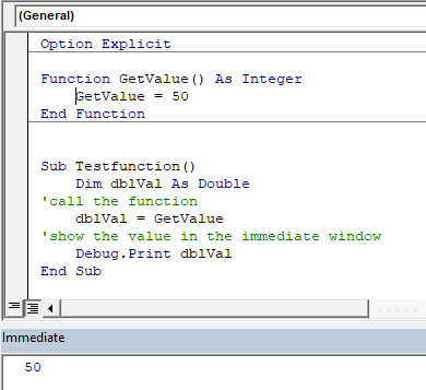
The value of 50 would always be returned.
You can also call the GetRange function from a Sub Procedure.
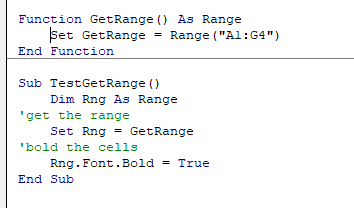
In the above example, the GetRange Function is called by the Sub Procedure to bold the cells in the range object.
Creating Functions
Single Argument
You can also assign a parameter or parameters to your function. These parameters can be referred to as Arguments.
Function ConvertKilosToPounds (dblKilo as Double) as Double
   ConvertKiloToPounds = dblKilo*2.2
End Function
We can then call the above function from a Sub Procedure in order to work out how many pounds a specific amount of kilos are.
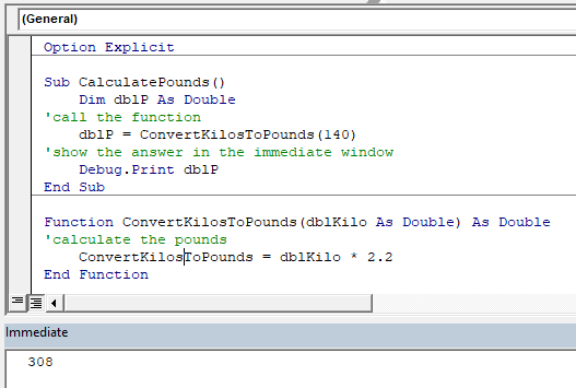
A function can be a called from multiple procedures within your VBA code if required. This is very useful in that it stops you from having to write the same code over and over again. It also enables you to divide long procedures into small manageable functions.
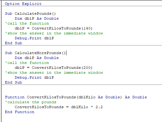
In the above example, we have 2 procedures – each of them are using the Function to calculate the pound value of the kilos passed to them in the dblKilo Argument of the function.
Multiple Arguments
You can create a Function with multiple arguments and pass the values to the Function by way of a Sub Procedure.
Function CalculateDayDiff(Date1 as Date, Date2 as Date) as Double
   CalculateDayDiff = Date2-Date1
End Function
We can then call the function to calculate the amount of days between 2 dates.
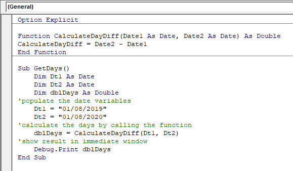
Optional Arguments
You can also pass Optional arguments to a Function. In other words, sometimes you may need the argument, and sometimes you may not – depending on what code you are using the Function with .
Function CalculateDayDiff(Date1 as Date, Optional Date2 as Date) as Double
'check for second date and if not there, make Date2 equal to today's date.
   If Date2=0 then Date2 = Date
'calculate difference
   CalculateDayDiff = Date2-Date1
End Function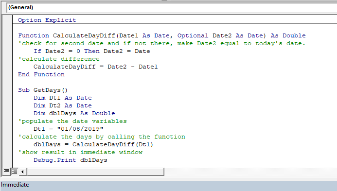
VBA Coding Made Easy
Stop searching for VBA code online. Learn more about AutoMacro — A VBA Code Builder that allows beginners to code procedures from scratch with minimal coding knowledge and with many time-saving features for all users!

Learn More
Default Argument Value
You can also set the default value of the Optional arguments when you are creating the function so that if the user omits the argument, the value that you have put as default will be used instead.
Function CalculateDayDiff(Date1 as Date, Optional Date2 as Date="06/02/2020") as Double
'calculate difference
   CalculateDayDiff = Date2-Date1
End Function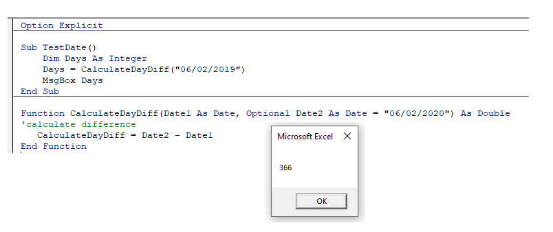
ByVal and ByRef
When you pass values to a function, you can use the ByVal or ByRef keywords. If you omit either of these, the ByRef is used as the default.
ByVal means that you are passing a copy of the variable to the function, whereas ByRef means you are referring to the original value of the variable. When you pass a copy of the variable (ByVal), the original value of the variable is NOT changed, but when you reference the variable, the original value of the variable is changed by the function.
Function GetValue(ByRef intA As Integer) As Integer
   intA = intA * 4
   GetValue = intA
End Function
In the function above, the ByRef could be omitted and the function would work the same way.
Function GetValue(intA As Integer) As Integer
   intA = intA * 4
   GetValue = intA
End Function
To call this function, we can run a sub-procedure.
Sub TestValues()
   Dim intVal As Integer
'populate the variable with the value 10
   intVal = 10
'run the GetValue function, and show the value in the immediate window
   Debug.Print GetValue(intVal)
'show the value of the intVal variable in the immediate window
   Debug.Print  intVal
End Sub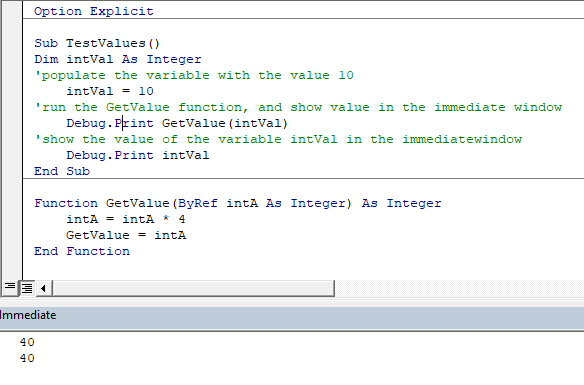
Note that the debug windows show the value 40 both times. When you pass the variable IntVal to the function – the value of 10 is passed to the function, and multiplied by 4. Using the ByRef keyword (or omitting it altogether), will AMEND the value of the IntVal variable. This is shown when you show first the result of the function in the immediate window (40), and then the value of the IntVal variable in the debug window (also 40).
If we do NOT want to change the value of the original variable, we have to use ByVal in the function.
Function GetValue(ByVal intA As Integer) As Integer
intA = intA * 4
GetValue = intA
End Function
Now if we call the function from a sub-procedure, the value of the variable IntVal will remain at 10.
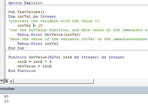
Exit Function
If you create a function that tests for a certain condition, and once the condition is found to be true, you want return the value from the function, you may need to add an Exit Function statement in your Function in order to exit the function before you have run through all the code in that function.
Function FindNumber(strSearch As String) As Integer
   Dim i As Integer
'loop through each letter in the string
   For i = 1 To Len(strSearch)
   'if the letter is numeric, return the value to the function
      If IsNumeric(Mid(strSearch, i, 1)) Then
         FindNumber= Mid(strSearch, i, 1)
   'then exit the function
         Exit Function
      End If
   Next
   FindNumber= 0
End Function
The function above will loop through the string that is provided until it finds a number, and then return that number from the string. It will only find the first number in the string as it will then Exit the function.
The function above can be called by a Sub routine such as the one below.
Sub CheckForNumber()
   Dim NumIs as Integer
'pass a text string to the find number function
   NumIs = FindNumber("Upper Floor, 8 Oak Lane, Texas")
'show the result in the immediate window
   Debug.Print NumIs
End Sub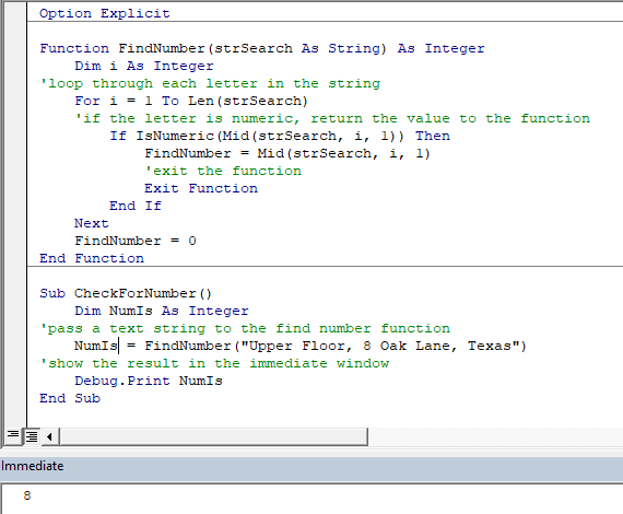
VBA Programming | Code Generator does work for you!
Using a Function from within an Excel Sheet
In addition to calling a function from your VBA code using a sub procedure, you can also call the function from within your Excel sheet. The functions that you have created should by default appear in your function list in the User Defined section of the function list.
Click on the fx to show the Insert Function dialog box.
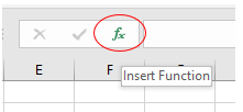
Select User Defined from the Category List
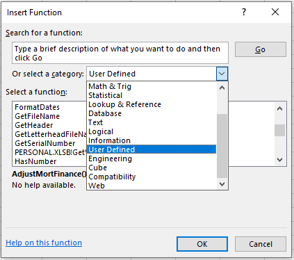
Select the function you require from the available User Defined Functions (UDF’s).

Alternatively, when you start writing your function in Excel, the function should appear in the drop down list of functions.
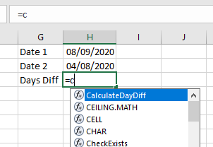
If you do not want the function to be available inside an Excel sheet, you need to put the Private word in front of the word Function when you create the function in your VBA code.
Private Function CalculateDayDiff(Date1 as Date, Date2 as Date) as Double
   CalculateDayDiff = Date2-Date1
End Function
It will now not appear in the drop down list showing the Excel functions available.
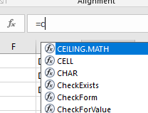
Interestingly enough, however, you can still use the function – it just will not appear in the list when looking for it!
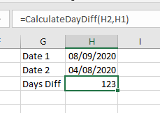
If you have declared the second argument as Optional, you can omit it within the Excel sheet as well as within the VBA code.
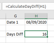
You can also use the a function that you have created without arguments in your Excel sheet.

Writing Your Own Functions In VBA
This page describes how to write your own worksheet functions in VBA.

While Excel provides a plethora of built-in functions, especially so if you include functions in the Analysis Took Pack
(in Excel 2007, the functions that used to be in the ATP are now native Excel functions) you may find it useful to create
your own custom function for things that Excel cannot (easily) do with the built-in functions. While it takes longer
for Excel to calculate a VBA function than it does to calculate a worksheet formula, all else being equal, the flexibility
of VBA often makes a VBA function the better choice. The rest of this page assumes that you are familiar with the
basics of VBA programming.
A User Defined Function (or UDF) is a Function procedure that typically (but not
necessarily) accepts some inputs and returns a result. A UDF can only return
a value to the cell(s) whence it was called — it must not modify the contents or formatting of any cell and must
not modify the operating environment of Excel. If you attempt to change anything, the function will terminate immediately and
return a #VALUE error to the calling cell. In Excel 97 and 2000, a UDF cannot use
the Find method of a Range object, even though that method does not
change anything in Excel. This was fixed with Excel 2002.
The following is an example of a simple UDF that calculates the area of a rectangle:
Function RectangleArea(Height As Double, Width As Double) As Double
    RectangleArea = Height * Width
End Function
This function takes as inputs two Double type variables, Height and Width,
and returns a Double as its result. Once you have defined the UDF in a code module, you can call it from a worksheet cell
with a formula like:
=RectangleArea(A1,B1)
where A1 and B1 contain the Height and Width of the rectangle.
Because functions take inputs and return a value, they are not displayed in the list of procedures in the Macros dialog.

The code for a UDF should be placed in a standard code module, not one of the Sheet modules and not
in the ThisWorkbook module. In the VBA editor, go to the Insert menu and choose Module.
This will insert a new code module into the project. A module can contain any number functions, so you can put many functions into
a single code module. You can change the name of a module from Module1 to something more meaningful
by pressing the F4 key to display the Properties window and changing the Name property
to whatever you want.
You can call a function from the same workbook by using just the function name. For example:
=RectangleArea(12,34)
It is possible, but strongly recommended against, to have two functions with the same name is two separate
code modules within the same workbook. You would call them using the module name from cells with formulas like:
=Module1.MyFunction(123)
=Module2.MyFunction(123)
Doing this will lead only to confusion, so just because it is possible doesn’t mean you should do it. Don’t do it.
Do not give the same name to both a module and a function (regardless of whether that module contains that function). Doing so
will cause an untrappable error.
You can call a UDF that is contained in another (open) workbook by using the workbook name in the formula. For example,
=’MyBook.xls’!RectangleArea(A1,A2)
will call the function RectangleArea defined in the workbook MyBook.xls.
If a function is defined in an Add-In (either an XLA or an Automation Add-In; see this page for
information about writing Automation Add-Ins in VB6), you don’t need to include the name of the Add-In file. The
function name alone is sufficient for calling a function in an Add-In.
CAUTION: Excel does not handle well the case when a workbook contains a
function with the same name as a function in an Add-In. Suppose both Book1.xls and
MyAddIn.xla have a function named Test defined as:
Function Test() As String
Test = ThisWorkbook.Name
End Function
The function Test in each workbook simply returns the name of the workbook in which the code resides,
so the function Test defined in Book1.xls returns the string
«Book1.xls» and the function Test defined in
MyAddIn.xla returns the string «MyAddIn.xla». In
Book1.xls, enter the formula =Test() in cell A1 and
enter the formula =MyAddin.xla!Test() in cell A2. The functions will work
properly when you first enter the formulas, but if you edit the formula in A2 (e.g., select the cell,
then press the F2 key followed by the ENTER key),
the name Test is recognized as a function in Book1.xls so Excel will
change the function call in cell A2 from =MyAddIn.xla!Test() to
simply =Test(), and this will call the function Test
from Book1.xls not MyAddIn.xla. This will almost certainly return an
incorrect result. This problem occurs only when the workbook and an Add-In both have a function with the same name. It does not
occurs if two workbooks have functions with the same name. This has not been fixed in Excel 2007.
As a general rule, you should pass into the function all the values it needs to properly calculate the result. That means that
your UDF should not make explicit refences to other cells. If you reference other cells directly from within the function,
Excel may not recalculate the function when that cell is changed. For example, a poorly written UDF is as follows:
Public Function BadRectangleArea(Height As Double) As Double
    BadRectangleArea = Height * Range("A1").Value
End Function
In this function, the Width is assumed to be in cell A1. The problem here is that Excel doesn’t know that
this function depends on cell A1 and therefore will not recalculate the formula when
A1 is changed. Thus, the cell calling the function call will not contain the correct result when
cell A1 is changed. You can force Excel to recalculate a UDF whenever any calculation is made by
adding the line
Application.Volatile True
as the first line in the function. For example,
Function BadRectangleArea(Height As Double) As Double
    Application.Volatile True
    BadRectangleArea = Height * Range("A1").Value
End Function
This has the drawback, however, that the function is recalculated even if it doesn’t need to be
recalculated, which can cause a performance problem. In general, you shouldn’t use Application.Volatile
but instead design your UDF to accept as inputs everything it needs to properly caclulate the result.
See the Returning Arrays From User Defined Functions page for information about returning
arrays as the result of your User Defined Function.
You can return an error value from a UDF if an incorrect input parameter is passed in. To do this, the function must return
a Variant data type and use the CVErr function to create an error-type Variant
result. For example, the function Divide below will return a #DIV/0 error if
the divisor is 0.
Function Divide(A As Double, B As Double) As Variant
    If B = 0 Then
        Divide = CVErr(xlErrDiv0)
    Else
        Divide = A / B
    End If
End Function
You can use any of the following error constants with the CVErr function to return an error to Excel:
- xlErrDiv0 for a #DIV/0 error
- xlErrNA for a #N/A error
- xlErrName for a #NAME? error
- xlErrNull for a #NULL error
- xlErrNum for a #NUM error
- xlErrRef for a #REF error
- xlErrValue for a #VALUE error
If any other value is passed to CVErr, Excel will treat it as a #VALUE error.
It is generally good practice to validate the input parameters and return an error value with CVErr rather
than letting the VBA code error out with #VALUE errors. If a run-time error occurs in your code, or you
attempt to change anything in Excel, such other cells, VBA terminates the function and returns a #VALUE
error to Excel.
Under nearly all circumstances, it is not necessary to know the actual address of the range from which your UDF was called. Indeed,
you should avoid have the need for such information. Your function should work the same regardless of where it was called from. However,
you may well need to know the size of the range from which your UDF was called if it was array entered into a range
of cells. The Application.Caller object will return a reference to the range from which your function
was called, regardless of whether that range is a single cell or a range of cells.
CAUTION: Application.Caller will be a Range object only when the function in which it appears
was called from a worksheet cell. If the function was called from another VB procedure, Application.Caller
will be an Error-type Variant and most any attempt to use it will result in a Type Mismatch (13) error. If the code containing
Application.Caller was called via the OnAction property of a Shape object on
a worksheet, Application.Caller will be a String containing the name of the sheet. Therefore, if your
function might be called from another VB procedure rather than only from a worksheet cell, you should test
Application.Caller with the IsObject function to ensure that it is indeed
an object before attempting to access any of its properties.
CAUTION: In Excel 2003, a new object, Application.ThisCell, was introduced. It is similar in nature to
Application.Caller, but differs when a UDF is array entered into a range of more than one cell.
Application.Caller will return the a Range reference to the entire range in which the UDF was array-entered.
Application.ThisCell returns a reference to the first (upper left) cell in the range from which the UDF
was called. Frankly, I’m not sure why Application.ThisCell was introduced in the first place.
You can get the properties of Application.Caller with code like the following:
    Function Test()
        Dim CallerRows As Long
        Dim CallerCols As Long
        Dim CallerAddr As String
        With Application.Caller
            CallerRows = .Rows.Count
            CallerCols = .Columns.Count
            CallerAddr = .Address
        End With
        Test = 1234
    End Function
You can define a function to accept a variable number of parameters in one of two somewhat different ways. You can use a specified
number of optional parameters, or you can allow the function to accept any number of parameters, including none at all, using
a ParamArray Variant parameter. The two methods are mutually exclusive. You cannot use both
optional parameters and a ParamArray in the same function.
Optional Variant Parameters
You can define one or more parameters as Optional Variant types. For example:
Function OptParam(D As Double, Optional B As Variant) As Variant
    If IsMissing(B) = True Then
        OptParam = D
    Else
        If IsNumeric(B) = True Then
            OptParam = D + B
        Else
            OptParam = CVErr(xlErrNum)
        End If
    End If
End Function
This function defines the parameter B as an optional Variant and uses the
IsMissing function to determine whether the parameter was passed. The IsMissing
function can be used only with Variant type parameters. If IsMissing is used
with any other data type (e.g., a Long), it will return False. More than
one parameter may be Optional, but those parameters must be the last parameters accepted by the function.
That is, once one parameter is specified as Optional, all the parameters that follow it must also be
optional. You cannot have a required parameter following an optional parameter. If a parameter is declared as Optional but is
not a Variant (e.g, it is a String or a Long) and that parameter is omitted,
the IsMissing function will return False and the default value for that
data type (0 or empty string) will be used. You can specify a default value for an optional parameter that should be used
if the parameter is omitted. For example, the parameter B in the function below is optional
with a default value of 2.
Function FF(A As Long, Optional B As Long = 2) As Variant
    If B = 0 Then
        FF = CVErr(xlErrDiv0)
    Else
        FF = A / B
    End If
End Function
In this code, the value 2 is used for the default value of B if B is omitted.
When using a default value for a parameter, you don’t call the IsMissing function. Your code should be
written to use either a passed in parameter value or the default value of the parameter.
With the code above, the following two worksheet functions are equivalent:
=FF(1,2)
=FF(1)
Variant ParamArray
The second method for working with optional parameters is to use a ParamArray Variant parameter.
A ParamArray allows any number of parameters, including none at all, to be passed to the function. You can
have one or more required parameters before the ParamArray, but you cannot have any optional
parameters if you have a ParamArray. Moreover, the ParamArray variable
must be the last parameter declared for a function. The ParamArray
variables must be Variant types. You cannot have a ParamArray of other types, such
as Long integers. If necessary, you should validate the values passed in the ParamArray,
such as to ensure they are all numeric. If your function requires one or more inputs followed by a variable number of parameters,
declare the required parameters explicitly and use a ParamArray only for the optional parameters.
For example, the function SumOf below accepts any number of inputs and simply adds them up:
Function SumOf(ParamArray Nums() As Variant) As Variant

    Dim N As Long
    Dim D As Double
    For N = LBound(Nums) To UBound(Nums)
        If IsNumeric(Nums(N)) = True Then
            D = D + Nums(N)
        Else
            SumOf = CVErr(xlErrNum)
            Exit Function
        End If
    Next N
    SumOf = D
End Function
In your function code, you can use:
Dim NumParams As Long
NumParams = UBound(Nums) — LBound(Nums) + 1
to determine how many parameters were passed in the ParamArray variable Nums. This will be 0 if
no parameters were passed as the ParamArray. Of course, the code above counts the number of
parameters within the ParamArray, not the total number of parameters to the function.
See Optional Paramateres To Procedures for a more in depth discussion of
Optional parameters and ParamArray parameter type.
Your function can return an array of values so that it can be entered as an array formula, either entered into an array of
cells or to return an array to be aggregated by a function like SUM. (See
this page for a discussion of Array Formulas.) The NumsUpTo function
below returns an array of the integers from 1 to the input parameter L. For simplicity,
L must be between 1 and 5. The function also requires that if the function is array entered, it
must be in either a single row or a single column. A range with more than one row and more than one column will result in
a #REF error. This restriction applies to this example only; it is not a limitation on UDF array
functions in general. See the next section for example code that return values to a two dimensional range of cells.
In a UDF, Application.Caller returns a Range type object that references the cell(s) from which
the formula was called. Using this, we can test whether we need a row array or a column array. If the function is called
from a column of cells (e.g., array entered into A1:A5), the VBA array must be transposed
before returning it to Excel. Note that there is also an object named Application.ThisCell that
references the cell from which a function is called. In functions called from a single cell,
Application.Caller and Application.ThisCell work the same. However, they
differ when a function is called as an array formula. You should use Application.Caller,
not Application.ThisCell.
Function NumsUpTo(L As Long) As Variant


Dim V() As Long
Dim ArraySize As Long
Dim N As Long
Dim ResultAsColumn As Boolean

If (L > 5) Or (L < 1) Then
    NumsUpTo = CVErr(xlErrValue)
    Exit Function
End If


If Application.Caller.Rows.Count > 1 And _
    Application.Caller.Columns.Count > 1 Then
        NumsUpTo = CVErr(xlErrRef)
        Exit Function
End If


If Application.Caller.Rows.Count > 1 Then
    ResultAsColumn = True
Else
    ResultAsColumn = False
End If


ReDim V(1 To L)


For N = 1 To UBound(V)
    V(N) = N
Next N

If ResultAsColumn = True Then
    NumsUpTo = Application.Transpose(V)
Else
    NumsUpTo = V
End If

End Function
If the SumUpTo function is called from a range that has more than one row, the array must
be transposed before it is returned, using the Application.Transpose function. The result of the
function is an array of L integers from 1 to L.
If the range from which the function is called has N cells, and N is less than L (the size
of the result array), elements at the end of array are discarded and only the firt N elements
are sent to the cells. If L is less than N (the function is entered into
an array of cells larger than L), #N/A errors fill out the ending
elements of the range on the worksheet. Since the result of NumsUpTo is an array, it can
be used in an array formula, such as
=SUM(NumsUpTo(5))
which returns 15, the sum of the numbers from 1 to 5.
To return an array to a range that contains more than one row and more than one column, create a two dimensional array
with the first dimension equal to the number of rows in the range and the second dimension equal to the number of columns in
the range. Then load that array, looping through the rows and columns and then return the array as the result.
The function AcrossThenDown below loads the calling cells with sequential integers, moving across
each row and then moving down to the next row. The function DownThenAcross below loads the
calling cells with sequential integers, moving down each column then moving right to the next column. The difference between
the two function is in the For loops, whether the outer loop is for Rows or Columns. As noted before,
use Application.Caller not Application.ThisCell to get a reference to the
range of cells calling the function.
Function AcrossThenDown() As Variant
    Dim NumCols As Long
    Dim NumRows As Long
    Dim RowNdx As Long
    Dim ColNdx As Long
    Dim Result() As Variant
    Dim N As Long

    NumCols = Application.Caller.Columns.Count
    NumRows = Application.Caller.Rows.Count


    ReDim Result(1 To NumRows, 1 To NumCols)

    For RowNdx = 1 To NumRows
        For ColNdx = 1 To NumCols
            N = N + 1
            Result(RowNdx, ColNdx) = N
        Next ColNdx
    Next RowNdx
    AcrossThenDown = Result
End Function


Function DownThenAcross() As Variant
    Dim NumCols As Long
    Dim NumRows As Long
    Dim RowNdx As Long
    Dim ColNdx As Long
    Dim Result() As Variant
    Dim N As Long


    NumCols = Application.Caller.Columns.Count
    NumRows = Application.Caller.Rows.Count


    ReDim Result(1 To NumRows, 1 To NumCols)

    For ColNdx = 1 To NumCols
        For RowNdx = 1 To NumRows
            N = N + 1
            Result(RowNdx, ColNdx) = N
        Next RowNdx
    Next ColNdx
    DownThenAcross = Result
End Function
This page last updated: 1-Sept-2007
Excel VBA Functions
We have seen that we can use the worksheet functions in VBA, i.e., the Excel worksheet functions in VBA coding using the Application.Worksheet method. But how do we use a function of VBA in Excel well? Such functions are called user-defined functions. When a user creates a function in VBA, we can use it in an Excel worksheet.
Although we have many functions in Excel to manipulate the data, sometimes we need to have some customization in the tools to save time as we do some tasks repeatedly. For example, we have predefined functions in excel like SUM, COUNTIFThe COUNTIF function in Excel counts the number of cells within a range based on pre-defined criteria. It is used to count cells that include dates, numbers, or text. For example, COUNTIF(A1:A10,”Trump”) will count the number of cells within the range A1:A10 that contain the text “Trump”
read more, SUMIFThe SUMIF Excel function calculates the sum of a range of cells based on given criteria. The criteria can include dates, numbers, and text. For example, the formula “=SUMIF(B1:B5, “<=12”)” adds the values in the cell range B1:B5, which are less than or equal to 12.
read more, COUNTIFS,”COUNTIFSread more VLOOKUPThe VLOOKUP excel function searches for a particular value and returns a corresponding match based on a unique identifier. A unique identifier is uniquely associated with all the records of the database. For instance, employee ID, student roll number, customer contact number, seller email address, etc., are unique identifiers.
read more, INDEX, MATCH in excelThe MATCH function looks for a specific value and returns its relative position in a given range of cells. The output is the first position found for the given value. Being a lookup and reference function, it works for both an exact and approximate match. For example, if the range A11:A15 consists of the numbers 2, 9, 8, 14, 32, the formula “MATCH(8,A11:A15,0)” returns 3. This is because the number 8 is at the third position.
read more, etc., but we do some tasks daily for which a single command or function is not available in Excel. Using VBA, we can create the User Defined Functions (UDFUser Defined Function in VBA is a group of customized commands created to give out a certain result. It is a flexibility given to a user to design functions similar to those already provided in Excel.read more) custom function.
Table of contents
- Excel VBA Functions
- What do VBA Functions do?
- How to Create Custom Functions using VBA?
- Example
- Step 1: Find Total Marks
- Step 2: Create ResultOfStudent Function
- Step 3: Apply ResultOfStudents Function to Get Result
- Step 4: Create ‘GradeForStudent’ Function to get Grades
- Example
- Recommended Articles
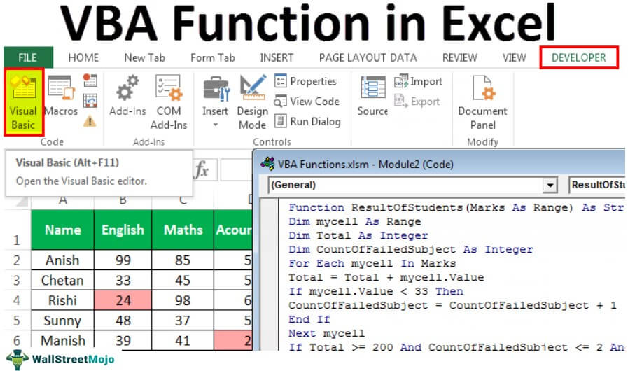
What do VBA Functions do?
- They carry out certain calculations; and
- Return a value
In VBA, while defining the function, we use the following syntax to specify the parameters and their data type.
Data type here is the type of dataData type is the core character of any variable, it represents what is the type of value we can store in the variable and what is the limit or the range of values which can be stored in the variable, data types are built-in VBA and user or developer needs to be aware which type of value can be stored in which data type. Data types assign to variables tells the compiler storage size of the variable.read more the variable will hold. It can hold any value (data type or class object).
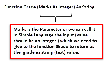
We can connect the object with its property or method using the period or dot (.) symbol.
How to Create Custom Functions using VBA?
You can download this VBA Function Excel Template here – VBA Function Excel Template
Example
Suppose we have the following data from a school where we need to find the total marks scored by the student, result, and grade.
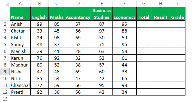
To sum up, the marks scored by an individual student in all subjects, we have an inbuilt function, SUM. But, determining the grade and result based on the criteria set out by the school is not available in Excel by default.
It is the reason why we need to create user-defined functions.
Step 1: Find Total Marks
First, we will find the total marks using the SUM function in excelThe SUM function in excel adds the numerical values in a range of cells. Being categorized under the Math and Trigonometry function, it is entered by typing “=SUM” followed by the values to be summed. The values supplied to the function can be numbers, cell references or ranges.read more.
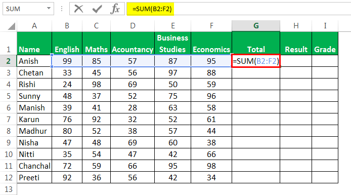
Then, press the “Enter” key to get the result.

Drag the formula to the rest of the cells.
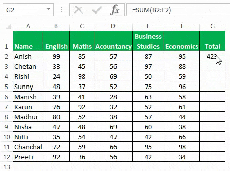
Now, to find out the result (passed, failed, or essential repeat), the criteria set by the school is that.
- Suppose a student has scored more than or equal to 200 as total marks out of 500. In addition, suppose they have also not failed in any subject (scored more than 32 in each subject), a student is passed.
- If the student scored more than or equal to 200 but failed in 1 or 2 subjects, then a student will get “Essential Repeat” in those subjects.
- If the student has scored either less than 200 or fails in 3 or more subjects, then the student failed.
Step 2: Create ResultOfStudent Function
To create a function named ‘ResultOfStudent,’ we need to open “Visual Basic Editor” by using any of the methods below:
- Using the Developer tab excel.Enabling the developer tab in excel can help the user perform various functions for VBA, Macros and Add-ins like importing and exporting XML, designing forms, etc. This tab is disabled by default on excel; thus, the user needs to enable it first from the options menu.read more
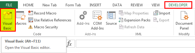
If the Developer tab is not available in MS Excel, then we can get that by using the following steps:
- Right-click anywhere on the ribbon. Then, choose to Customize the Ribbon in excelRibbons in Excel 2016 are designed to help you easily locate the command you want to use. Ribbons are organized into logical groups called Tabs, each of which has its own set of functions.read more‘.
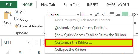
When we choose this command, the “Excel Options” dialog box opens.
- We need to check the box for “Developer” to get the tab.
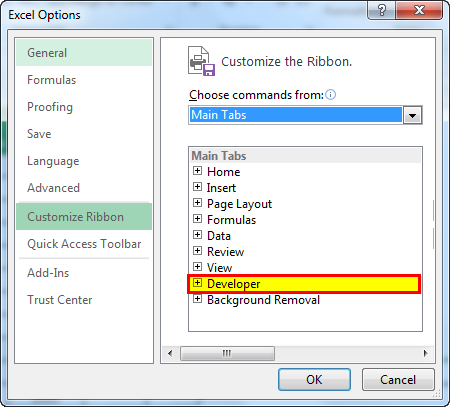
- Using the shortcut key, Alt+F11.

- When we open the VBA editorThe Visual Basic for Applications Editor is a scripting interface. These scripts are primarily responsible for the creation and execution of macros in Microsoft software.read more, we need to insert the module by going to the Insert menu and choosing a module.

- We need to paste the following code into the module.
Function ResultOfStudents(Marks As Range) As String

Dim mycell As Range
Dim Total As Integer
Dim CountOfFailedSubject As Integer

For Each mycell In Marks
Total = Total + mycell.Value

If mycell.Value < 33 Then
CountOfFailedSubject = CountOfFailedSubject + 1
End If

Next mycell
If Total >= 200 And CountOfFailedSubject <= 2 And CountOfFailedSubject > 0 Then
ResultOfStudents = "Essential Repeat"

ElseIf Total >= 200 And CountOfFailedSubject = 0 Then
ResultOfStudents = "Passed"

Else
ResultOfStudents = "Failed"
End If

End Function
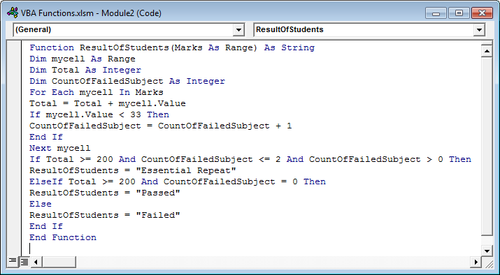
The above function returns the result for a student.
We need to understand how this code is working.
The first statement, ‘Function ResultOfStudents(Marks As Range) As String,’ declares a function named ‘ResultOfStudents’ that will accept a range as input for marks and return the result as a string.
Dim mycell As Range
Dim Total As Integer
Dim CountOfFailedSubject As Integer
These three statements declare variables, i.e.,
- ‘myCell’ as a Range,
- ‘Total’ as Integer (to store total marks scored by a student),
- ‘‘CountOfFailedSubject’ is an Integer (to store the number of subjects a student has failed).
For Each mycell In Marks
Total = Total + mycell.Value

If mycell.Value < 33 Then
CountOfFailedSubject = CountOfFailedSubject + 1
End If

Next mycell
This code checks for every cell in the ‘Marks’ range. It adds the value of every cell in the ‘Total’ variable. If the cell’s value is less than 33, add 1 to the ‘CountOfFailedSubject’ variable.
If Total >= 200 And CountOfFailedSubject <= 2 And CountOfFailedSubject > 0 Then
ResultOfStudents = "Essential Repeat"

ElseIf Total >= 200 And CountOfFailedSubject = 0 Then
ResultOfStudents = "Passed"

Else
ResultOfStudents = "Failed"
End If
This code checks the value of ‘Total’ and ‘CountOfFailedSubject’ and passes the ‘Essential Report,’ ‘Passed,’ or ‘Failed’ to the ‘ResultOfStudents.’
Step 3: Apply ResultOfStudents Function to Get Result
ResultOfStudents function takes marks, i.e., selecting 5 marks scored by the student.
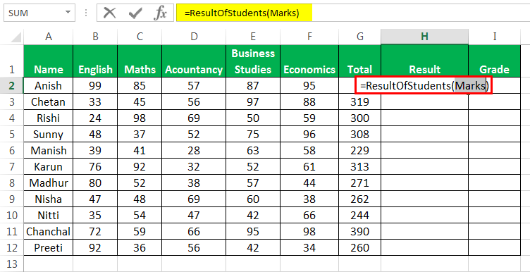
Now, select the range of cells, B2: F2.
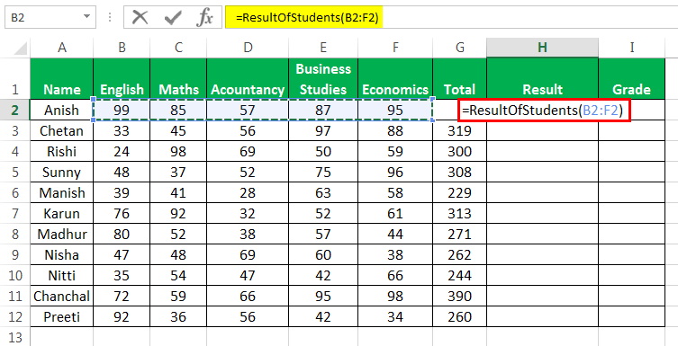
Drag the formula to the rest of the cells.
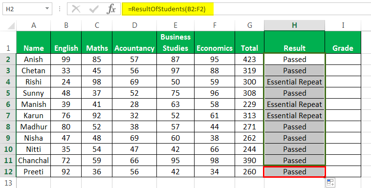
Step 4: Create ‘GradeForStudent’ Function to get Grades
Now to find out the grade for the student, we will create one more function named ‘GradeForStudent.’
The code would be:
Function GradeForStudent(TotalMarks As Integer, Result As String) As String

If TotalMarks > 440 And TotalMarks <= 500 And ((Result = "Passed" Or Result = "Essential Repeat")
Or Result = "Essential Repeat") Then GradeForStudent = "A"

ElseIf TotalMarks > 380 And TotalMarks <= 440 And (Result = "Passed" Or Result = "Essential Repeat") Then
GradeForStudent = "B"

ElseIf TotalMarks > 320 And TotalMarks <= 380 And (Result = "Passed" Or Result = "Essential Repeat") Then
GradeForStudent = "C"

ElseIf TotalMarks > 260 And TotalMarks <= 320 And (Result = "Passed" Or Result = "Essential Repeat") Then
GradeForStudent = "D"

ElseIf TotalMarks >= 200 And TotalMarks <= 260 And (Result = "Passed" Or Result = "Essential Repeat") Then
GradeForStudent = "E"

ElseIf TotalMarks < 200 Or Result = "Failed" Then
GradeForStudent = "F"

End If

End Function
This function assigns a ‘Grade’ to the student based on the ‘Total Marks’ and ‘Result.’
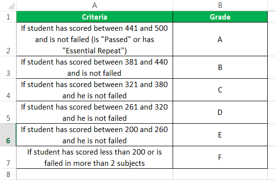
We need to write the formula and open the brackets in cell H2. Press Ctrl+Shift+A to find out the arguments.

The GradeForStudent function takes Total marks (sum of marks) and the result of the student as an argument to calculate the grade.
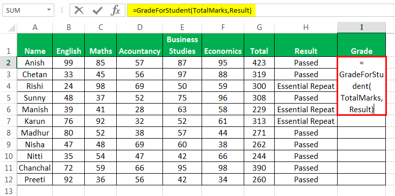
Now, select the individual cells, G2 and H2.
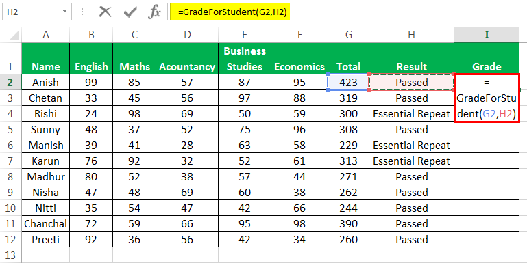
Now, we need to press Ctrl+D after selecting the cells to copy down the formulas.
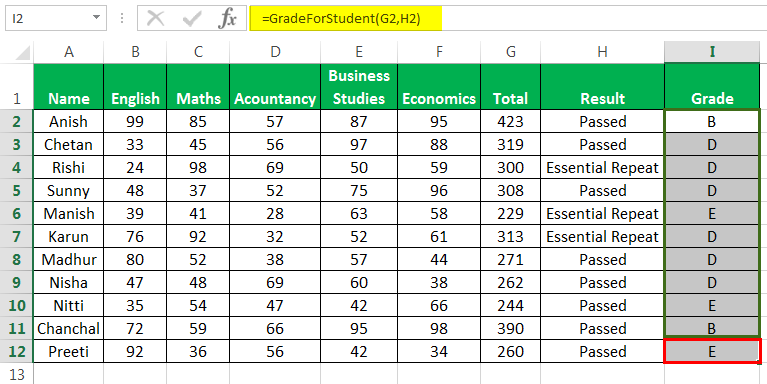
We can highlight the values of less than 33 with the red background color to find out the subjects in which the student failed.

Recommended Articles
This article is a guide to VBA Functions. Here, we discuss creating custom functions using VBA code, practical examples, and a downloadable Excel template. You may learn more about VBA from the following articles:-
- VBA IIFThe «VBA IIF» condition evaluates the supplied expression or logical test and returns TRUE or FALSE as a result.read more
- SUMIF With VLOOKUPSUMIF is used to sum cells based on some condition, which takes arguments of range, criteria, or condition, and cells to sum. When there is a large amount of data available in multiple columns, we can use VLOOKUP as the criteria.read more
- Excel SUMIF Between Two DatesWhen we wish to work with data that has serial numbers with different dates and the condition to sum the values is based between two dates, we use Sumif between two dates. read more
- Excel VBA Delete RowIn VBA, to delete the command and to delete any rows together, the trick is that we give a single row reference if we need to delete a single row. However, for the multiple columns, we can provide numerous row references.read more
Создание пользовательской функции в VBA Excel, ее синтаксис и компоненты. Описание пользовательской функции и ее аргументов. Метод Application.MacroOptions.
Пользовательская функция — это процедура VBA, которая производит заданные вычисления и возвращает полученный результат. Используется для вставки в ячейки рабочего листа Excel или для вызова из других процедур.
Объявление пользовательской функции
Синтаксис функции
|
[Static] Function Имя ([СписокАргументов])[As ТипДанных] [Операторы] [Имя = выражение] [Exit Function] [Операторы] [Имя = выражение] End Function |
Компоненты функции
- Static — необязательное ключевое слово, указывающее на то, что значения переменных, объявленных в функции, сохраняются между ее вызовами.
- Имя — обязательный компонент, имя пользовательской функции.
- СписокАргументов — необязательный компонент, одна или более переменных, представляющих аргументы, которые передаются в функцию. Аргументы заключаются в скобки и разделяются между собой запятыми.
- Операторы — необязательный компонент, блок операторов (инструкций).
- Имя = выражение — необязательный* компонент, присвоение имени функции значения выражения или переменной. Обычно, значение присваивается функции непосредственно перед выходом из нее.
- Exit Function — необязательный компонент, принудительный выход из функции, если ей уже присвоено окончательное значение.
*Один из компонентов Имя = выражение следует считать обязательным, так как если не присвоить функции значения, смысл ее использования теряется.
Видимость функции
Видимость пользовательской функции определяется необязательными ключевыми словами Public и Private, которые могут быть указаны перед оператором Function (или Static, в случае его использования).
Ключевое слово Public указывает на то, что функция будет доступна для вызова из других процедур во всех модулях открытых книг Excel. Функция, объявленная как Public, отображается в диалоговом окне Мастера функций.
Ключевое слово Private указывает на то, что функция будет доступна для вызова из других процедур только в пределах программного модуля, в котором она находится. Функция, объявленная как Private, не отображается в диалоговом окне Мастера функций, но ее можно ввести в ячейку вручную.
Если ключевое слово Public или Private не указано, функция считается по умолчанию объявленной, как Public.
Чтобы пользовательская функция всегда была доступна во всех открытых книгах Excel, сохраните ее в Личной книге макросов без объявления видимости или как Public. Но если вы планируете передать рабочую книгу с пользовательской функцией на другой компьютер, код функции должен быть в программном модуле передаваемой книги.
Пример пользовательской функции
Для примера мы рассмотрим простейшую пользовательскую функцию, которой в следующем параграфе добавим описание. Называется функция «Деление», объявлена с типом данных Variant, так как ее возвращаемое значение может быть и числом, и текстом. Аргументы функции — Делимое и Делитель — тоже объявлены как Variant, так как в ячейках Excel могут быть числовые значения разных типов, и функция IsNumeric тоже проверяет разные типы данных и требует, чтобы ее аргументы были объявлены как Variant.
|
Function Деление(Делимое As Variant, Делитель As Variant) As Variant If IsNumeric(Делимое) = False Or IsNumeric(Делитель) = False Then Деление = «Ошибка: Делимое и Делитель должны быть числами!» Exit Function ElseIf Делитель = 0 Then Деление = «Ошибка: деление на ноль!» Exit Function Else Деление = Делимое / Делитель End If End Function |
Эта функция выполняет деление значений двух ячеек рабочего листа Excel. Перед делением проверяются два блока условий:
- Если делимое или делитель не являются числом, функция возвращает значение: «Ошибка: Делимое и Делитель должны быть числами!», и производится принудительный выход из функции оператором Exit Function.
- Если делитель равен нулю, функция возвращает значение: «Ошибка: деление на ноль!», и производится принудительный выход из функции оператором Exit Function.
Если проверяемые условия не выполняются (возвращают значение False) производится деление чисел и функция возвращает частное (результат деления).
Вы можете скопировать к себе в стандартный модуль эту функцию и она станет доступна в разделе «Определенные пользователем» Мастера функций. Попробуйте вставить функцию «Деление» в ячейку рабочего листа с помощью Мастера и поэкспериментируйте с ней.
Практического смысла функция «Деление» не имеет, но она хорошо демонстрирует как объявляются, создаются и работают пользовательские функции в VBA Excel. А еще она поможет продемонстрировать, как добавлять к функциям и аргументам описания. С полноценной пользовательской функцией вы можете ознакомиться здесь.
Добавление описания функции
В списке функций, выводимом Мастером, невозможно добавить или отредактировать их описание. Список макросов позволяет добавлять процедурам описание, но в нем нет функций. Проблема решается следующим образом:
- Запустите Мастер функций, посмотрите, как отображается имя нужной функции и закройте его.
- Откройте список макросов и в поле «Имя макроса» впишите имя пользовательской функции.
- Нажмите кнопку «Параметры» и в открывшемся окне добавьте или отредактируйте описание.
- Нажмите кнопку «OK», затем в окне списка макросов — «Отмена». Описание готово!
Добавление описания на примере функции «Деление»:

Добавление описания пользовательской функции
Описание функции «Деление» в диалоговом окне Мастера функций «Аргументы функции»:

Описание пользовательской функции в окне «Аргументы функции»
С помощью окна «Список макросов» можно добавить описание самой функции, а ее аргументам нельзя. Но это можно сделать, используя метод Application.MacroOptions.
Метод Application.MacroOptions
Метод Application.MacroOptions позволяет добавить пользовательской функции описание, назначить сочетание клавиш, указать категорию, добавить описания аргументов и добавить или изменить другие параметры. Давайте рассмотрим возможности этого метода, используемые чаще всего.
Пример кода с методом Application.MacroOptions:
|
Sub ИмяПодпрограммы() Application.MacroOptions _ Macro:=«ИмяФункции», _ Description:=«Описание функции», _ Category:=«Название категории», _ ArgumentDescriptions:=Array(«Описание 1», «Описание 2», «Описание 3», ...) End Sub |
- ИмяПодпрограммы — любое уникальное имя, подходящее для наименования процедур.
- ИмяФункции — имя функции, параметры которой добавляются или изменяются.
- Описание функции — описание функции, которое добавляется или изменяется.
- Название категории — название категории в которую будет помещена функция. Если параметр Category отсутствует, пользовательская функция будет записана в раздел по умолчанию — «Определенные пользователем». Если указанное Название категории соответствует одному из названий стандартного списка, функция будет записана в него. Если такого Названия категории нет в списке, будет создан новый раздел с этим названием и функция будет помещена в него.
- «Описание 1», «Описание 2», «Описание 3», … — описания аргументов в том порядке, как они расположены в объявлении пользовательской функции.
Эта подпрограмма запускается один раз, после чего ее можно удалить или использовать как шаблон для корректировки параметров других пользовательских функций.
Сейчас с помощью метода Application.MacroOptions попробуем изменить описание пользовательской функции «Деление» и добавить описания аргументов.
|
Sub ИзменениеОписания() Application.MacroOptions _ Macro:=«Деление», _ Description:=«Описание функции Деление изменено методом Application.MacroOptions», _ ArgumentDescriptions:=Array(«- любое числовое значение», «- числовое значение, кроме нуля») End Sub |
После однократного запуска этой подпрограммы получаем следующий результат:

Новое описание пользовательской функции и ее второго аргумента
Метод Application.MacroOptions не работает в Личной книге макросов, но и здесь можно найти решение. Добавьте описания к пользовательским функциям и их аргументам в обычной книге Excel, затем экспортируйте модуль с функциями в любой каталог на жестком диске и оттуда импортируйте в Личную книгу макросов. Все описания сохранятся.