Why is the focus of this VBA tutorial the FormulaR1C1 property instead of the Range.Formula property?
To answer these (and similar questions) you may have, let’s take a look at:
R1C1-Style References And The FormulaR1C1 Property: Why Are They Important And Useful
In Chapter 5 of Excel 2016 VBA and Macros, Excel authorities Bill Jelen (Mr. Excel) and Tracy Syrstad provide a very good introduction to the historical background of the A1 and R1C1 referencing styles. The short story, as explained at ExcelMate, is roughly as follows:
- #1: Back in the early days of spreadsheets, VisiCalc (the first spreadsheet program) introduced the A1 notation. Lotus 1-2-3, a very popular spreadsheet program in the 1980s, followed suit and also used A1-style references.
#2: Microsoft’s Multiplan (an early spreadsheet program from Microsoft) used the R1C1-style notation.
#3: Lotus 1-2-3 was very popular during the 1980s.
#4: Eventually, as explained here, Microsoft added A1-style references. As explained in Excel 2016 VBA and Macros:
Officially (…), Microsoft supports both styles of addressing.
For most practical purposes, nobody (or virtually nobody) uses the R1C1-style of referencing when working with Excel. However, when working with VBA, this isn’t the case.
For starters, as I show at the beginning of this post, the Macro Recorder constantly uses the Range.FormulaR1C1 property. Therefore, having a good understanding of R1C1 references allows you to read the code that the Macro Recorder creates.
However, this isn’t the main strength of the R1C1-style notation. Here’s the deal:
When you’re working with Visual Basic for Applications, R1C1-style references allow you to (for most purposes) create more efficient and powerful VBA applications. Additionally, if you want to be able to use certain features, you must use the R1C1-style notation. In the words of Mr. Excel and Tracy Syrstad (in Excel 2016 VBA and Macros):
I have to give Microsoft credit. R1C1-style formulas, you’ll grow to understand, are actually more efficient, especially when you are dealing with writing formulas in VBA. Using R1C1-style addressing enables you to write more efficient code. Plus, there are some features such as setting up array formulas that require you to enter a formula in R1C1 style.
At Chandoo.org, you can find some additional reasons why (as a general matter) you understanding the R1C1-style notation is helpful. This includes, for example, the fact that the R1C1 style may help you when working with VBA loops.
All of the above doesn’t mean that you must always use R1c1-style notation when working with Visual Basic for Applications. There are several Excel experts and power users who have (at different times) expressed that they don’t necessarily rely on the R1C1 style all the time.
Furthermore, as I explain below, there are cases where you can rely on the A1-style notation while working with VBA.
Given this, you might still wonder whether the R1C1-style notation is really more efficient than the A1 style when working with Visual Basic for Applications.
Fortunately, you don’t need to take my (or Mr. Excel’s) word. Let’s take a closer look at the R1C1-style notation to see some evidence of this:
R1C1-Style Notation: How Are Cell References Created
In a previous section, I provide an introductory explanation of how you can create cell references that use the R1C1 style. At the most basic level, you can refer to any cell by using the R1C1-style notation by concatenating the following 4 elements:
- Element #1: The letter “R”.
Element #2: The reference to the number of the row where the cell is.
Element #3: The letter “C”.
I provide some introductory examples of cell references above.
When working with Excel, you can encounter (and use) 3 different types of cell references. This applies regardless of whether you’re using the A1 or the R1C1-style notation. These 3 types of cell references, as explained at office.com, are:
- Type #1: Relative references.
Relative references change as you copy a formula from one cell to another.
When you’re working with A1-style references, relative references are the default. For example, when creating a relative reference to refer to the first cell of a worksheet using A1-style notation, you simply write “A1”.
Type #2: Absolute references.
Absolute references don’t change as you copy a formula from one cell to another.
As explained in the Excel 2016 Bible, absolute references use 2 dollar signs ($). One of the dollar signs ($) goes before the column identifier. The other dollar sign ($) is placed before the row identifier. Therefore, to create an absolute reference to the first cell of a worksheet using A1-style notation, you type “$A$1”.
Type #3: Mixed references.
As implied by their name, mixed references are a mix of relative and absolute references. Therefore, if you’re using mixed references, either the row or the column is absolute (doesn’t change as you copy the formula from one cell to another) and the other is relative (changes as you copy the formula).
Mixed references use a single dollar sign ($). This dollar sign is placed prior to the identifier of the item (row or column) that is absolute. For example, if you’re creating a mixed reference to the first cell of a worksheet: (i) “$A1” results in a mixed reference where the column (A) is absolute and the row (1) is relative, and (ii) “A$1” results in a reference where the column (A) is relative and the row (1) is absolute.
If you’re interested in learning more about relative, absolute and mixed cell references when using the A1-style notation, the following resources may be of interest to you:
- Switch between relative, absolute, and mixed references at office.com.
Since the focus of this VBA tutorial is the R1C1-style notation, let’s take a look at how you create relative, absolute and mixed references with it:
Relative Reference With R1C1-Style Notation
It might sound crazy, but:
At its most basic level, the way in which you build relative references using the R1C1-style notation (which I explain in this section) is the main reason why R1C1-style references allow you to make your VBA code more efficient. So, even though the R1C1-style reference examples I provide below may look relatively simple, be patient. The sample Sub procedure I provide below, shows how you can use the R1C1-style notation and the Range.FormulaR1C1 property to efficiently set formulas in Excel.
Note also that, despite the usefulness of the R1C1-style notation, there are some issues you should keep in mind when creating macros that rely on such notation. I provide a thorough explanation of this topic towards the end of this blog post.
Relative references are the default in the R1C1-style notation.
R1C1-style relative references have square brackets ([ ]) around the numbers of the rows and columns.
However, relative R1C1-style references are subject to additional rules. To understand most of this, it may help if you think of relative references in the R1C1-style notation being built in the following 3 steps:
Step #1: Start On The Active Cell
Imagine that you’re currently in cell R10C5. When using A1-style notation, this is cell E10.

This cell is the base (or reference) for the relative reference you’re building.
Step #2: Move A Certain Number Of Rows Up Or Down
You specify the row of the cell you’re referring to by moving a certain number of rows up or down. For these purposes you count from the cell you’re working on (the current active cell).
The number of rows you’re moving up or down determines the number that goes after the letter “R” in an R1C1-style reference. More precisely:
- If you use a positive number, you’re moving down the worksheet.

If you use a negative number, you’re moving up the worksheet.

For example, if you’re in cell R10C5 and you want to refer to the cell immediately below it (R11C5), the first portion of the cell reference is “R[1]”.
However, if you’re referring to the cell immediately above R10C5, the first portion of the cell reference is “R[-1]”.
Finally, if you’re referring to the cell itself (creating a circular reference), the first portion of the cell reference is simply “R”.
Step #3: Move A Certain Number Of Columns To The Right Or To The Left
The rules for specifying the column to which you’re referring to are a reflection of the rules I explain above to refer to the row number. Here’s what I mean:
- You specify the column of the cell you’re referring to by moving a certain number of columns to the right or to the left of the cell you’re working on.
The number of columns you move to the right or to the left determines the number that goes after the letter “C” in the R1C1-style reference.
Positive numbers mean you’re moving to the right along the worksheet.

Negative numbers mean you’re moving to the left along the worksheet.

Continuing with the same example as in the previous step #2, if you’re in cell R10C5 and want to refer to the cell to the right, the second portion of the cell reference is “C[1]”. To refer to the cell to the left of R10C5, the second portion of the reference is “C[-1]”. To refer to the cell itself (and create a circular reference), the first portion of the cell reference is “C” alone.
Let’s take a look at 4 examples of relative R1C1-style references:
Example #1 Of R1C1-Style Relative Reference
If you’re working on the first cell of the worksheet (R1C1, or A1 in A1-style notation) and want to refer to cell R8C5 (E8 in A1-style notation, you move:
- 7 rows down; and
Therefore, the reference is “R[7]C[4]”.

Example #2 Of R1C1-Style Relative Reference
If the current active cell is R5C5 (E5 in A1-style notation) and want to refer to cell R2C2 (B2 in A1-style notation), you move:
As a consequence of this, the reference is “R[-3]C[-3]”.

Example #3 Of R1C1-Style Relative Reference
If you’re in cell R10C5 (E10 in A1-style notation) and want to refer to cell R4C7 (G4 in A1-style notation), you move:
Therefore, the reference is “R[6]C[2]”.

Example #4 Of R1C1-Style Relative Reference
If you’re in cell R8C4 (cell D8 in A1-style notation) and want to refer to cell R2C4, you move:
Therefore, the reference is “R[-6]C”.

You probably get the idea. Therefore, let’s move on to…
Absolute References With R1C1-Style Notation
To build absolute references with R1C1-style notation, simply do the opposite of what you do when building relative references. That is, omit the square brackets ([ ]).
This is the style that I use above when introducing the R1C1-style notation.
For example, when creating an absolute R1C1-style reference to the first cell in a worksheet, type “R1C1”.
Mixed References With R1C1-Style Notation
To build mixed references using the R1C1-style notation, include the square brackets ([ ]) around the number of the item (row or column) you want to make relative. In other words:
- To build a mixed R1C1-style reference where the row is relative and the column is absolute, surround the row number with square brackets ([ ]).
Such a mixed reference looks roughly like “R[#]C#”.
To create a mixed R1C1-style reference in which the row is absolute and the column is relative, wrap the column number with square brackets ([ ]).
In this case, the mixed references look roughly like “R#C[#]”.
Let’s go back to example #1 of a relative reference using the R1C1-style notation to see how a relative R1C1-style reference looks like:
In that situation, the active cell is R1C1 (A1 in A1-style notation). You’re referring to cell R8C5 (E8 in A1-style notation). The relative reference in such a situation is R[7]C[4].
In such a case, you can build the following 2 mixed references:
- Reference #1: R8C[4]. In this case, the row is absolute and the column is relative.

Reference #2: R[7]C5. In this reference, the row is relative and the column is absolute.

Referring To A Full Row Or Column Using R1C1-Style Notation
To create a reference to all the cells within a particular row or column, simply omit the other item (row or column) of the reference. What I mean is the following:
- To refer to a full row, omit the column identifier. Such a R1C1-style reference is of the form “R[#]” (if relative) or “R#” (if absolute).
The rules regarding relative and absolute references, and the respective use of square brackets ([ ]) continues to be the same as I explain in the previous sections.
For example, R5 is an absolute reference to row 5.

Similarly, if the active cell is R1C1, C[4] refers to the full column located 4 columns to the right or R1C1 (column 5). This is a relative reference.

Now that you have a good grasp of the R1C1-style notation, let’s take a look at the…
Range.FormulaR1C1 Property
One of the topics of focus of this VBA tutorial is the Range.FormulaR1C1 property. Let’s take a look at its main characteristics:
Range.FormulaR1C1: Basic Description And Purpose
Range.FormulaR1C1 is a read/write property. Therefore, you can both (i) read the property or (ii) modify it.
The main purpose of the FormulaR1C1 property depends on whether you’re reading or modifying the property. More precisely:
- If you’re fetching the current setting of the property, Range.FormulaR1C1 returns the formula (using R1C1-style notation) of the relevant range.
The Range.FormulaR1C1 property uses the language of the macro. Therefore, the returned formula (when reading) or the set formula (when writing) are both in that language. If you’re interested in dealing with R1C1-style formulas in the language of the user, you may be interested in learning about the Range.FormulaR1C1Local property (which I explain below).
Range.FormulaR1C1: Syntax
The basic syntax of the Range.FormulaR1C1 property is as follows:
“expression” is a variable representing a Range object.
Range.FormulaR1C1: Reading The Property
When you use the Range.FormulaR1C1 property for purposes of returning the formula of a particular range, the exact behavior of the property varies slightly depending on the contents of the relevant range. More precisely, as explained at the Microsoft Dev Center:
- If a cell contains a constant, Formula R1C1 returns the constant.
If the cell is empty, FormulaR1C1 returns an empty string.
Range.FormulaR1C1: Working With Ranges
If you use the Range.FormulaR1C1 property to set the formula of a multiple-cell range, Excel fills all the cells of the relevant range with the formula. Generally, as I show below, Excel adjusts the cell references automatically.
You can see how the FormulaR1C1 property works with multi-cell ranges in practice by taking a look at the practical examples below.
Range.FormulaR1C1: Setting A Date
If you use the Range.FormulaR1C1 property to set the value or formula of a particular cell to a date, Excel proceeds as follows:
- Step #1: It checks whether the cell you’re working with is formatted using a date or time number format.
Step #2: If the condition is met, and the cell already uses a date or time number format, Excel leaves the format untouched.
However, if the cell isn’t formatted using a date or time number format, Excel sets the format of the cell to be the default short date number format.
Range.FormulaR1C1Local Property And Language Considerations
As explained by Excel authorities Dick Kusleika and Mike Alexander in Excel 2016 Power Programming with VBA:
In general, you need not be concerned with the language in which you write your VBA code.
The reason for this, as explained by Kusleika and Alexander, is that Excel uses 2 object libraries:
- Excel’s object library.
Excel always sets the English version of both libraries as the default. This is the case regardless of which language you use in Excel.
Working with formulas is, generally, one of the exceptions to the above rule. In other words, if you’re working in a particular VBA application whose users may have different language settings, language compatibility may be an issue you should consider.
Let’s take a closer look at this point:
Excel Formulas And Language Considerations
As a general matter, Excel functions are localized. As a consequence, the name of a particular function, such as IFERROR varies depending on the language in which Excel runs. Let me explain what I mean:
In this blog post, I explain several text functions such as LEFT, RIGHT, MID, LEN, FIND and SEARCH. These, however, are the names used by the English version of Excel. The names of the functions change depending on the particular language you’re using Excel in.
The following table shows the names of these particular functions in 10 different languages. I prepared the translation using the Excel-Translator.
| #1 | English | LEFT | RIGHT | MID | LEN | FIND | SEARCH |
| #2 | Spanish | IZQUIERDA | DERECHA | EXTRAE | LARGO | ENCONTRAR | HALLAR |
| #3 | German | LINKS | RECHTS | TEIL | LÄNGE | FINDEN | SUCHEN |
| #4 | French | GAUCHE | DROITE | STXT | NBCAR | TROUVE | CHERCHE |
| #5 | Dutch | LINKS | RECHTS | DEEL | LENGTE | VIND.ALLES | VIND.SPEC |
| #6 | Italian | SINISTRA | DESTRA | STRINGA.ESTRAI | LUNGHEZZA | TROVA | RICERCA |
| #7 | Portuguese (Brazil) | ESQUERDA | DIREITA | EXT.TEXTO | NÚM.CARACT | PROCURAR | LOCALIZAR |
| #8 | Polish | LEWY | PRAWY | FRAGMENT.TEKSTU | DŁ | ZNAJDŹ | SZUKAJ.TEKST |
| #9 | Danish | VENSTRE | HØJRE | MIDT | LÆNGDE | FIND | SØG |
| #10 | Turkish | SOLDAN | SAĞDAN | PARÇAAL | UZUNLUK | BUL | MBUL |
Excel MVP Mourad Louha is an expert in this topic and has invested a substantial amount of time and resources in the development of the Excel-Translator. Mourad explains the challenge when working with Excel functions in a multilingual setting quite clearly as follows:
If you send your Excel file to someone using a different language for Excel than you, the functions and formulas used in the workbook are automatically translated by Excel when opening the file. However, the automatic translation usually does not work, if you directly insert foreign language formulas into your worksheet.
When working with the FormulaR1C1 property, you fall within the second scenario (in bold). In other words:
If you’re reading or setting a formula by using the FormulaR1C1 VBA property, the functions are usually not automatically translated.
The easiest way to deal with language compatibility concerns when working with the FormulaR1C1 property is to use the local version of the FormulaR1C1 property:
Range.FormulaR1C1Local Property
To understand why the LanguageR1C1Local may be helpful, let’s go back to what I say above about the language used by the Range.FormulaR1C1. That is, the FormulaR1C1 property uses the language of the macro.
On the other hand, the Range.FormulaR1C1Local property, which I cover in this section, uses the language of the user.
For practical purposes, other than this important aspect, all of the comments I make above regarding the Range.FormulaR1C1 property are applicable. More precisely:
- Range.FormulaR1C1Local is a read/write property.
You can use Range.FormulaR1C1Local to return (read) or set (write) the formula of a range using R1C1-style notation.
The basic syntax of Range.FormulaR1C1Local is “expression.FormulaR1C1Local”.
“expression” represents a Range object.
The item returned by Range.FormulaR1C1Local (when used for reading purposes) depends on whether the cell (i) is empty, (ii) contains a constant, or (iii) contains a formula.
I explain further details of this behavior above.
When you use the Range.FormulaR1C1Local property to set a value or formula to a date: (i) Excel checks whether the cell is formatted using a date or time number format and (ii) sets the format to the default short date number format if the cell isn’t formatted as a date or time.
- When working with the FormulaR1C1 property and reading this tutorial, bear in mind the following:
#1: Range.FormulaR1C1 uses the language of the macro.
#2: Range.FormulaR1C1Local uses the language of the user.
Range.FormulaR1C1 Property Example: Setting The Formula Of A Cell Range To Create A Table
This Excel VBA R1C1-Style Notation and FormulaR1C1 Property Tutorial is accompanied by an Excel workbook containing the data and macros I use. You can get immediate free access to this example workbook by subscribing to the Power Spreadsheets Newsletter.
For this example, let’s assume that you want to want to prepare a table that shows different combinations of the total revenue generated by 2 different revenue streams. The revenue generated by these streams is listed in $100 increments in the following cell ranges:
- C5 (R5C3 in R1C1-style notation) to CX5 (R5C102 in R1C1-style notation).

In order to fill the table and show the different total revenue combinations, you must add the following 2 numbers in each cell:
- The value at the top of the relevant column (in row 5); and
Setting up the formula manually is relatively straightforward. You can do this in the following 2 easy steps:
- Step #1: Enter the relevant formula in the first cell of the table.
In this particular case, the formula I enter is “=SUM(C$5,$B6)”. Notice that the cell references are mixed: (i) in C$5, the row number is absolute and, therefore, isn’t adjusted when the formula is copied to other cells, and (ii) in $B6, the column number is absolute and isn’t adjusted as the formula is copied and pasted.

Step #2: Copy the formula and paste it in all the relevant cells of the table.
As expected, the table is filled with the appropriate formulas. Notice, for example, how the formula in cell O29 appropriately adds the cell at the top of the column (O5) and at the beginning of the row (B29).

The following screenshot shows some of the formulas within this worksheet. Notice how Excel (pretty much) rewrites a portion of the formula for each cell in order to adjust the cell references.

In the words of Mr. Excel and Tracy Syrstad (in Excel 2016 VBA and Macros):
It seems intimidating to consider having a macro enter all these different formulas.
The reason for this, however, is because the formulas in the screenshots above use A1-style notation.
The following screenshot shows the same portion of the table we’re working on as that above. The only difference is that, in the image below, R1C1-style notation is used.

Notice that, when using R1C1-style notation, all of the formulas in the table are exactly the same.
As I explain above, you can use the Range.FormulaR1C1 property to enter such a formula in such a range.
The following sample macro (FormulaR1C1_Table) achieves this:

This Sub procedure consists of a single statement:
Let’s take a look at its 3 main components separately to understand how the macro works:

Item #1: Range(“C6:CX105”)
This makes reference to the Application.Range property. Within the syntax of the FormulaR1C1 property that I introduce above, this item takes the place of the expression that returns a Range object.
More precisely, this statement returns the range of cells from C6 to CX105 of the current active worksheet.
The fully qualified reference is “Application.ActiveSheet.Range(“C6:CX105”). However, as I explain on this VBA tutorial about Excel’s Object Model, you can simplify the reference by assuming the following default objects:
Item #2: FormulaR1C1 =
This item makes reference to the FormulaR1C1 property.
As I explain in the tutorial about VBA Object Properties, whenever you’re setting a property value, you use an equal sign (=) to separate the property name (FormulaR1C1) from the property value (item #3 below).
Item #3: “=SUM(R5C,RC2)”
This item is the value that is set for the FormulaR1C1 property of all the cells within the range returned by item #1 above. This formula is the one I show in the screenshot above.
The following GIF shows what happens when I execute the sample FormulaR1C1_Table macro. Notice how, as expected, Excel appropriately fills all the cells within the table.

Let’s make an additional check by reviewing the formula of cell O29. Notice that, in this case, the formula is exactly the same as that which resulted from the manual process I show above (=SUM(O$5,$B29)).

Considering all that I’ve said throughout this VBA tutorial regarding the advantages of using R1C1-style notation and the Range.FormulaR1C1 property when working with VBA, you may be surprised by what I explain in the following section:
Setting The Formula Of A Cell Range To Create A Table With The Range.Formula Property
Strictly speaking, you can replicate the results of the sample FormulaR1C1_Table macro above by using A1-style notation and the Range.Formula property.
The focus of this particular blog post isn’t the Range.Formula property. I may cover this topic in a future tutorial. If you want to be notified whenever I publish new content in Power Spreadsheets, please register for our Newsletter by entering your email address below:
As explained by Excel expert Andrew Poulsom at MrExcel.com, the Range.Formula property behaves very similarly to the Range.FormulaR1C1 property I explain above. In other words, you can use the Formula property to either:
- Return (read) the formula (using A1-style notation) of the range you’re working with.
So, for purposes of this explanation, the Range.Formula and Range.FormulaR1C1 properties achieve the same purpose with 1 basic difference:
The FormulaR1C1 property uses R1C1-style notation. The Formula property uses A1-style notation.
The following sample macro (Formula_Table) is the equivalent of the FormulaR1C1_Table example macro above.

The single statement in the Sub procedure is substantially the same. The only 2 differences between the 2 macros are the following:

- Difference #1: FormulaR1C1_Table uses the Range.FormulaR1C1 property. Formula_Table uses the Range.Formula property.
Difference #2: As a consequence of the above, the formula set by FormulaR1C1_Table uses R1C1-style notation. The formula set by Formula_Table uses A1-style notation.
Note that, in this particular case, the formula that I use in the VBA code is that corresponding to the first cell of the table (cell C6). As I explain further below, Excel automatically adjusts the formula for the other cells in the table.
The following GIF shows the what happens in Excel when I execute the sample Formula_Table macro. Notice that the results are substantially the same as those obtained when executing the FormulaR1C1_Table macro above.

You can also check the formula in cell O29 again (as I did above). The formula is exactly the same as that obtained when carrying out the process manually or executing the FormulaR1C1_Table macro (=SUM(O$5,$B29)).

The reason for this, as explained in Excel 2016 VBA and Macros, is that Excel actually carries out the following 3 steps whenever you enter an A1-style formula:
- Step #1: Converts the A1-style formula to an R1C1-style formula, as I explain above.
Step #2: Enters the converted R1C1-style formula in the entire range.
The consequence of this is that the macro roughly mirrors the manual process that I explain above. That 2-step process is as follows:
- Step #1: The relevant formula is entered in the first cell of the table (cell C6).
So, strictly speaking, you can use both the FormulaR1C1 and the Formula properties to enter a formula in a particular range of cells.
Macros That Rely On Relative References: Avoid This Error
In a previous section, I provide a thorough explanation of how to use relative references when working with the R1C1-style notation.
When working with macros for purposes of creating relative references, there’s a particular behavior that you need to be aware of as it can be the source of mistakes. This is more thoroughly explained by experts Bill Jelen (Mr. Excel) and Tracy Syrstad in Excel 2016 VBA and Macros.
To understand how this can happen, let’s go back to the example I provide at the beginning of this blog post. At that point, I enter numbers 1 through 5 in cells B5 to B9.

For the sake of this example, I create the following sample macro (FormulaR1C1_Error).

This sample macro proceeds as follows:
- Step #1: Uses the Application.ActiveCell property to return the current active cell.
This macro isn’t extremely useful for practical purposes. I’m just using it to get a point across
The following GIF shows what happens when I execute the macro while the active cell is cell C10. Notice that, as expected, Excel enters a reference to the cell located 5 rows above and 1 column to the left of C10. That is cell B5, whose value is 1.

The macro works properly. If you execute the macro for the 4 cells below cell C10 (C11 to C14), the macro enters references to the values that are already entered in cells B6 to B9.
However, take a look at what happens when I execute this macro while the active cell is A5:

Notice that Excel doesn’t return an error. It rather makes reference to cell XFD1048576.

What’s the bottom line?
In such situation, Excel goes around the worksheet. Therefore:
- If your macro makes reference to a cell that is “above” row 1, Excel wraps around and goes to the last row of the worksheet to continue searching for the referred cell.
In the example above, both things of these things happened:
- The macro created a reference to a cell 1 row “above” row 1. Once Excel wraps around, this results in the last row of the worksheet (row 1,048,576 in recent Excel versions).
The consequence of all of this is that Excel creates the reference that appears in the screenshot above to cell XFD1048576.
I assume that, unless you’re facing a very particular situation or scenario, this isn’t the behavior you want from your macros.
Conclusion
If you’ve completed this VBA tutorial, you now have enough knowledge to start using the R1C1-style notation and the Range.FormulaR1C1 property for purposes of making your Excel macros more efficient, flexible and powerful. Among other topics, you know:
- What are the A1 and the R1C1-style notations.
Why are the R1C1-style notation and the FormulaR1C1 property useful and important.
How you can create absolute, relative and mixed references when working with the R1C1-style, and a particular behavior that you should take into consideration when creating relative references within VBA to avoid potential mistakes.
What are the main characteristics of the Formula.R1C1 property.
In addition to the above, you’ve seen a practical example showing how you can use the Range.FormulaR1C1 (or alternatively the Range.Formula) property for purposes of specifying the formula of a large range of cells.
This Excel VBA R1C1-Style Notation and FormulaR1C1 Property Tutorial is accompanied by an Excel workbook containing the data and macros I use above. You can get immediate free access to this example workbook by subscribing to the Power Spreadsheets Newsletter.
Источник
In this Article
- Formulas in VBA
- Macro Recorder and Cell Formulas
- VBA FormulaR1C1 Property
- Absolute References
- Relative References
- Mixed References
- VBA Formula Property
- VBA Formula Tips
- Formula With Variable
- Formula Quotations
- Assign Cell Formula to String Variable
- Different Ways to Add Formulas to a Cell
- Refresh Formulas
This tutorial will teach you how to create cell formulas using VBA.
Formulas in VBA
Using VBA, you can write formulas directly to Ranges or Cells in Excel. It looks like this:
Sub Formula_Example()

    'Assign a hard-coded formula to a single cell
    Range("b3").Formula = "=b1+b2"

    'Assign a flexible formula to a range of cells
    Range("d1:d100").FormulaR1C1 = "=RC2+RC3"

End Sub
There are two Range properties you will need to know:
- .Formula – Creates an exact formula (hard-coded cell references). Good for adding a formula to a single cell.
- .FormulaR1C1 – Creates a flexible formula. Good for adding formulas to a range of cells where cell references should change.
For simple formulas, it’s fine to use the .Formula Property. However, for everything else, we recommend using the Macro Recorder…
Macro Recorder and Cell Formulas
The Macro Recorder is our go-to tool for writing cell formulas with VBA. You can simply:
- Start recording
- Type the formula (with relative / absolute references as needed) into the cell & press enter
- Stop recording
- Open VBA and review the formula, adapting as needed and copying+pasting the code where needed.
I find it’s much easier to enter a formula into a cell than to type the corresponding formula in VBA.
Notice a couple of things:
- The Macro Recorder will always use the .FormulaR1C1 property
- The Macro Recorder recognizes Absolute vs. Relative Cell References
VBA FormulaR1C1 Property
The FormulaR1C1 property uses R1C1-style cell referencing (as opposed to the standard A1-style you are accustomed to seeing in Excel).
Here are some examples:
Sub FormulaR1C1_Examples()

    'Reference D5 (Absolute)
    '=$D$5
    Range("a1").FormulaR1C1 = "=R5C4"

    'Reference D5 (Relative) from cell A1
    '=D5
    Range("a1").FormulaR1C1 = "=R[4]C[3]"

    'Reference D5 (Absolute Row, Relative Column) from cell A1
    '=D$5
    Range("a1").FormulaR1C1 = "=R5C[3]"

    'Reference D5 (Relative Row, Absolute Column) from cell A1
    '=$D5
    Range("a1").FormulaR1C1 = "=R[4]C4"

End Sub
Notice that the R1C1-style cell referencing allows you to set absolute or relative references.
Absolute References
In standard A1 notation an absolute reference looks like this: “=$C$2”. In R1C1 notation it looks like this: “=R2C3”.
To create an Absolute cell reference using R1C1-style type:
- R + Row number
- C + Column number
Example: R2C3 would represent cell $C$2 (C is the 3rd column).
    'Reference D5 (Absolute)
    '=$D$5
    Range("a1").FormulaR1C1 = "=R5C4"
Relative References
Relative cell references are cell references that “move” when the formula is moved.
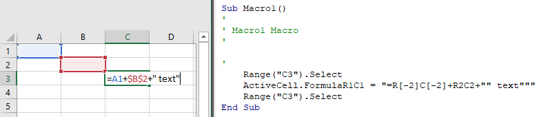
In standard A1 notation they look like this: “=C2”. In R1C1 notation, you use brackets [] to offset the cell reference from the current cell.
Example: Entering formula “=R[1]C[1]” in cell B3 would reference cell D4 (the cell 1 row below and 1 column to the right of the formula cell).
Use negative numbers to reference cells above or to the left of the current cell.
    'Reference D5 (Relative) from cell A1
    '=D5
    Range("a1").FormulaR1C1 = "=R[4]C[3]"
Mixed References
Cell references can be partially relative and partially absolute. Example:
    'Reference D5 (Relative Row, Absolute Column) from cell A1
    '=$D5
    Range("a1").FormulaR1C1 = "=R[4]C4"
VBA Coding Made Easy
Stop searching for VBA code online. Learn more about AutoMacro — A VBA Code Builder that allows beginners to code procedures from scratch with minimal coding knowledge and with many time-saving features for all users!

Learn More
VBA Formula Property
When setting formulas with the .Formula Property you will always use A1-style notation. You enter the formula just like you would in an Excel cell, except surrounded by quotations:
    'Assign a hard-coded formula to a single cell
    Range("b3").Formula = "=b1+b2"
VBA Formula Tips
Formula With Variable
When working with Formulas in VBA, it’s very common to want to use variables within the cell formulas. To use variables, you use & to combine the variables with the rest of the formula string. Example:
Sub Formula_Variable()
    Dim colNum As Long
    colNum = 4

    Range("a1").FormulaR1C1 = "=R1C" & colNum & "+R2C" & colNum

End Sub
VBA Programming | Code Generator does work for you!
Formula Quotations
If you need to add a quotation (“) within a formula, enter the quotation twice (“”):
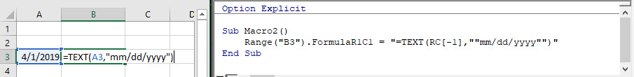
Sub Macro2()
    Range("B3").FormulaR1C1 = "=TEXT(RC[-1],""mm/dd/yyyy"")"
End Sub
A single quotation (“) signifies to VBA the end of a string of text. Whereas a double quotation (“”) is treated like a quotation within the string of text.
Similarly, use 3 quotation marks (“””) to surround a string with a quotation mark (“)
MsgBox """Use 3 to surround a string with quotes"""
' This will print <"Use 3 to surround a string with quotes"> immediate window
Assign Cell Formula to String Variable
We can read the formula in a given cell or range and assign it to a string variable:
'Assign Cell Formula to Variable
Dim strFormula as String
strFormula = Range("B1").Formula
Different Ways to Add Formulas to a Cell
Here are a few more examples for how to assign a formula to a cell:
- Directly Assign Formula
- Define a String Variable Containing the Formula
- Use Variables to Create Formula
Sub MoreFormulaExamples ()
' Alternate ways to add SUM formula
' to cell B1
'
  Dim strFormula as String
  Dim cell as Range
  dim fromRow as long, toRow as long

  Set cell = Range("B1")

  ' Directly assigning a String
  cell.Formula = "=SUM(A1:A10)"

  ' Storing string to a variable
  ' and assigning to "Formula" property
  strFormula = "=SUM(A1:A10)"
  cell.Formula = strFormula

  ' Using variables to build a string
  ' and assigning it to "Formula" property
  fromRow = 1
  toRow   = 10
  strFormula = "=SUM(A" & fromValue & ":A" & toValue & ")
  cell.Formula = strFormula
End Sub
Refresh Formulas
As a reminder, to refresh formulas, you can use the Calculate command:
CalculateTo refresh single formula, range, or entire worksheet use .Calculate instead:
Sheets("Sheet1").Range("a1:a10").Calculate If you’ve used the macro recorder, you’re probably familiar with both R1C1-style notation and the FormulaR1C1 property. This is because, as explained at Stack Overflow, the macro recorder constantly uses FormulaR1C1.
For example, even though you normally use the Range.Value property for purposes of entering a value in a cell, the macro recorder uses the Range.FormulaR1C1 property for those same purposes. To give you an idea, I used the macro recorder for purposes of creating the following sample macro (Enter_Value_FormulaR1C1). I recorded my actions while (i) entering numbers 1 through 5 in cells B5 to B9 and (ii) selecting cell B10 at the end.

Notice how the macro recorder uses the FormulaR1C1 property every single time.

As explained in Excel 2016 Power Programming with VBA and by Bob Phillips at excelforum.com, you normally use the Range.Value property for purposes of entering a value in a cell. In practice, using FormulaR1C1 “produces the same result”.
However, my focus on this particular VBA tutorial isn’t comparing the Range.FormulaR1C1 property with the Range.Value property. My focus is the Range.FormulaR1C1 property itself and the R1C1-style notation.
More particularly, my purpose with this blog post is to provide you with all the information you need to understand and use both the R1C1-style notation and the Range.FormulaR1C1 property.
You might be wondering whether you should take the time to learn about these 2 topics.
If that’s the case, you can refer to the section below where I explain why R1C1-style references and the Range.FormulaR1C1 property are useful. For the moment, and to make it short, my opinion is that you should take the time to learn and understand both the R1C1-style notation and the FormulaR1C1 property because, as explained by Excel authorities Bill Jelen (Mr. Excel) and Tracy Syrstad in Excel 2016 VBA and Macros:
Taking 30 minutes to understand R1C1 will make every macro you write for the rest of your life easier to code.
The following table of contents lists the main sections of this Excel tutorial:
Now, let’s start by taking a look at…
R1C1-Style And A1-Style Notation: A Basic Introduction
In order to understand the rest of this Excel tutorial, and how the FormulaR1C1 property may help you when working with VBA, having a good understanding of R1C1 notation is useful. I provide an introduction to the R1C1 notation in this section.
First, let me explain what I mean by “notation”:
When working with Excel formulas, notation is (in broad terms) the system you use to represent a cell reference. When referring to a cell in Excel, you usually create the reference by taking into consideration the following 2 items:
- Column.
- Row.
If you’ve been working with Excel for a while, you’re probably quite familiar with the most common notation:
A1-Style Notation
The A1 reference style is Excel’s default style notation.
As explained by Microsoft, when you build a cell reference using the A1 reference style, you:
- Refer to the column by using the letter that appears in the column heading. In recent Excel versions, this letter can be from A to XFD.

- Refer to the row by using the number that appears in the row heading. In recent Excel versions, this number ranges from 1 to 1,048,576.


When using the A1-style notation, you create a cell reference by concatenating the column letter and the row number. For example:
- “A1” refers to the first cell in the worksheet, where column A and row 1 intersect.

- “C5” refers to the cell at the intersection of column C and row 5.

- “E10” makes reference to the cell where column E and row 10 intersect.

- …
- And so on. You probably get the idea.


In other words, A1-style notation is simply the cell reference style you’re used to working with in Excel.
With this basic knowledge of what notation and the A1-style notation are, we can take a closer look at:
R1C1-Style Notation
R1C1-style notation is the alternative reference style to the A1-style notation I explain in the previous section.
The main difference between the A1 and R1C1 notations is the way in which columns are identified. Here’s what I mean:
- When you’re using the A1-style notation, columns are identified by letters. I explain this in the previous section.
- When you’re working with R1C1-style references, columns are identified by numbers. In recent Excel versions, this number can be from 1 to 16,384.


What’s the bottom line?
Well, as explained by Microsoft, in the R1C1-style notation:
Both the rows and the columns on the worksheet are numbered.
A second, also important, difference between the A1 and R1C1 styles is the way in which you identify rows and columns when building cell references. As I mention above, when you’re working with the A1 system, you create a reference by concatenating (i) the column identifier and (ii) the row identifier.
When you’re working the R1C1-style references, 2 things change:
- #1: The order in which you concatenate the rows and columns. Therefore:
If you’re working with A1-style references, (i) the column goes first and (ii) the row goes second.
If you’re using the R1C1 style, you concatenate the rows and columns in the opposite order. That is: (i) the row goes first and (ii) the column goes second.
- #2: The way in which you identify the relevant rows and columns. What I mean is the following:
If you’re using the A1 style, you concatenate the column letter and the row number. This is what I explain in the previous section.
If you’re working with the R1C1-style notation: (i) the column number is preceded by the letter “C” and (ii) the row number is preceded by the letter “R”.
Let’s see how this looks like in practice:
- “R1C1” refers to the cell at the intersection of the first column and the first row. In A1-style notation (as I explain above) you refer to this cell as A1.

- “R5C3” makes reference to the cell where the fifth row and the third column intersect. In the example that I provide in the previous section (using the A1 style), you call this cell C5.

- “R10C5” is the cell where the tenth row and the fifth column intersect. When working with A1-style references, this is cell E10.


Now that you understand the R1C1-style notation, you may be wondering things such as:
- Why is the R1C1 style useful?
- Why is the focus of this VBA tutorial the FormulaR1C1 property instead of the Range.Formula property?
- Why should you understand R1C1-style references and the FormulaR1C1 property when working with VBA?
To answer these (and similar questions) you may have, let’s take a look at:
R1C1-Style References And The FormulaR1C1 Property: Why Are They Important And Useful
In Chapter 5 of Excel 2016 VBA and Macros, Excel authorities Bill Jelen (Mr. Excel) and Tracy Syrstad provide a very good introduction to the historical background of the A1 and R1C1 referencing styles. The short story, as explained at ExcelMate, is roughly as follows:
- #1: Back in the early days of spreadsheets, VisiCalc (the first spreadsheet program) introduced the A1 notation. Lotus 1-2-3, a very popular spreadsheet program in the 1980s, followed suit and also used A1-style references.
- #2: Microsoft’s Multiplan (an early spreadsheet program from Microsoft) used the R1C1-style notation.
- #3: Lotus 1-2-3 was very popular during the 1980s.
- #4: Eventually, as explained here, Microsoft added A1-style references. As explained in Excel 2016 VBA and Macros:
Officially (…), Microsoft supports both styles of addressing.
For most practical purposes, nobody (or virtually nobody) uses the R1C1-style of referencing when working with Excel. However, when working with VBA, this isn’t the case.
For starters, as I show at the beginning of this post, the Macro Recorder constantly uses the Range.FormulaR1C1 property. Therefore, having a good understanding of R1C1 references allows you to read the code that the Macro Recorder creates.
However, this isn’t the main strength of the R1C1-style notation. Here’s the deal:
When you’re working with Visual Basic for Applications, R1C1-style references allow you to (for most purposes) create more efficient and powerful VBA applications. Additionally, if you want to be able to use certain features, you must use the R1C1-style notation. In the words of Mr. Excel and Tracy Syrstad (in Excel 2016 VBA and Macros):
I have to give Microsoft credit. R1C1-style formulas, you’ll grow to understand, are actually more efficient, especially when you are dealing with writing formulas in VBA. Using R1C1-style addressing enables you to write more efficient code. Plus, there are some features such as setting up array formulas that require you to enter a formula in R1C1 style.
At Chandoo.org, you can find some additional reasons why (as a general matter) you understanding the R1C1-style notation is helpful. This includes, for example, the fact that the R1C1 style may help you when working with VBA loops.
All of the above doesn’t mean that you must always use R1c1-style notation when working with Visual Basic for Applications. There are several Excel experts and power users who have (at different times) expressed that they don’t necessarily rely on the R1C1 style all the time.
Furthermore, as I explain below, there are cases where you can rely on the A1-style notation while working with VBA.
Given this, you might still wonder whether the R1C1-style notation is really more efficient than the A1 style when working with Visual Basic for Applications.
Fortunately, you don’t need to take my (or Mr. Excel’s) word. Let’s take a closer look at the R1C1-style notation to see some evidence of this:
R1C1-Style Notation: How Are Cell References Created
In a previous section, I provide an introductory explanation of how you can create cell references that use the R1C1 style. At the most basic level, you can refer to any cell by using the R1C1-style notation by concatenating the following 4 elements:
- Element #1: The letter “R”.
- Element #2: The reference to the number of the row where the cell is.
- Element #3: The letter “C”.
- Element #4: The reference to the number of the cell’s column.
I provide some introductory examples of cell references above.
When working with Excel, you can encounter (and use) 3 different types of cell references. This applies regardless of whether you’re using the A1 or the R1C1-style notation. These 3 types of cell references, as explained at office.com, are:
- Type #1: Relative references.
Relative references change as you copy a formula from one cell to another.
When you’re working with A1-style references, relative references are the default. For example, when creating a relative reference to refer to the first cell of a worksheet using A1-style notation, you simply write “A1”.
- Type #2: Absolute references.
Absolute references don’t change as you copy a formula from one cell to another.
As explained in the Excel 2016 Bible, absolute references use 2 dollar signs ($). One of the dollar signs ($) goes before the column identifier. The other dollar sign ($) is placed before the row identifier. Therefore, to create an absolute reference to the first cell of a worksheet using A1-style notation, you type “$A$1”.
- Type #3: Mixed references.
As implied by their name, mixed references are a mix of relative and absolute references. Therefore, if you’re using mixed references, either the row or the column is absolute (doesn’t change as you copy the formula from one cell to another) and the other is relative (changes as you copy the formula).
Mixed references use a single dollar sign ($). This dollar sign is placed prior to the identifier of the item (row or column) that is absolute. For example, if you’re creating a mixed reference to the first cell of a worksheet: (i) “$A1” results in a mixed reference where the column (A) is absolute and the row (1) is relative, and (ii) “A$1” results in a reference where the column (A) is relative and the row (1) is absolute.
If you’re interested in learning more about relative, absolute and mixed cell references when using the A1-style notation, the following resources may be of interest to you:
- Switch between relative, absolute, and mixed references at office.com.
- Cell References at Excel Easy.
- Relative And Absolute Cell References at GCFLearnFree.org.
Since the focus of this VBA tutorial is the R1C1-style notation, let’s take a look at how you create relative, absolute and mixed references with it:
Relative Reference With R1C1-Style Notation
It might sound crazy, but:
At its most basic level, the way in which you build relative references using the R1C1-style notation (which I explain in this section) is the main reason why R1C1-style references allow you to make your VBA code more efficient. So, even though the R1C1-style reference examples I provide below may look relatively simple, be patient. The sample Sub procedure I provide below, shows how you can use the R1C1-style notation and the Range.FormulaR1C1 property to efficiently set formulas in Excel.
Note also that, despite the usefulness of the R1C1-style notation, there are some issues you should keep in mind when creating macros that rely on such notation. I provide a thorough explanation of this topic towards the end of this blog post.
Relative references are the default in the R1C1-style notation.
R1C1-style relative references have square brackets ([ ]) around the numbers of the rows and columns.
However, relative R1C1-style references are subject to additional rules. To understand most of this, it may help if you think of relative references in the R1C1-style notation being built in the following 3 steps:
Step #1: Start On The Active Cell
Imagine that you’re currently in cell R10C5. When using A1-style notation, this is cell E10.
This cell is the base (or reference) for the relative reference you’re building.
Step #2: Move A Certain Number Of Rows Up Or Down
You specify the row of the cell you’re referring to by moving a certain number of rows up or down. For these purposes you count from the cell you’re working on (the current active cell).
The number of rows you’re moving up or down determines the number that goes after the letter “R” in an R1C1-style reference. More precisely:
- If you use a positive number, you’re moving down the worksheet.

- If you use a negative number, you’re moving up the worksheet.
- If you use no number at all, you move neither up nor down.
For example, if you’re in cell R10C5 and you want to refer to the cell immediately below it (R11C5), the first portion of the cell reference is “R[1]”.
However, if you’re referring to the cell immediately above R10C5, the first portion of the cell reference is “R[-1]”.
Finally, if you’re referring to the cell itself (creating a circular reference), the first portion of the cell reference is simply “R”.
Step #3: Move A Certain Number Of Columns To The Right Or To The Left
The rules for specifying the column to which you’re referring to are a reflection of the rules I explain above to refer to the row number. Here’s what I mean:
- You specify the column of the cell you’re referring to by moving a certain number of columns to the right or to the left of the cell you’re working on.
- The number of columns you move to the right or to the left determines the number that goes after the letter “C” in the R1C1-style reference.
- Positive numbers mean you’re moving to the right along the worksheet.
- Negative numbers mean you’re moving to the left along the worksheet.
- No number means you’re staying on the same column.
Continuing with the same example as in the previous step #2, if you’re in cell R10C5 and want to refer to the cell to the right, the second portion of the cell reference is “C[1]”. To refer to the cell to the left of R10C5, the second portion of the reference is “C[-1]”. To refer to the cell itself (and create a circular reference), the first portion of the cell reference is “C” alone.
Let’s take a look at 4 examples of relative R1C1-style references:
Example #1 Of R1C1-Style Relative Reference
If you’re working on the first cell of the worksheet (R1C1, or A1 in A1-style notation) and want to refer to cell R8C5 (E8 in A1-style notation, you move:
- 7 rows down; and
- 4 columns to the right.
Therefore, the reference is “R[7]C[4]”.
Example #2 Of R1C1-Style Relative Reference
If the current active cell is R5C5 (E5 in A1-style notation) and want to refer to cell R2C2 (B2 in A1-style notation), you move:
- 3 rows up; and
- 3 rows to the left.
As a consequence of this, the reference is “R[-3]C[-3]”.
Example #3 Of R1C1-Style Relative Reference
If you’re in cell R10C5 (E10 in A1-style notation) and want to refer to cell R4C7 (G4 in A1-style notation), you move:
- 6 rows up; and
- 2 columns to the right.
Therefore, the reference is “R[6]C[2]”.
Example #4 Of R1C1-Style Relative Reference
If you’re in cell R8C4 (cell D8 in A1-style notation) and want to refer to cell R2C4, you move:
- 6 rows up, and
- Stay in the same column.
Therefore, the reference is “R[-6]C”.
You probably get the idea. Therefore, let’s move on to…
Absolute References With R1C1-Style Notation
To build absolute references with R1C1-style notation, simply do the opposite of what you do when building relative references. That is, omit the square brackets ([ ]).
This is the style that I use above when introducing the R1C1-style notation.
For example, when creating an absolute R1C1-style reference to the first cell in a worksheet, type “R1C1”.
Mixed References With R1C1-Style Notation
To build mixed references using the R1C1-style notation, include the square brackets ([ ]) around the number of the item (row or column) you want to make relative. In other words:
- To build a mixed R1C1-style reference where the row is relative and the column is absolute, surround the row number with square brackets ([ ]).
Such a mixed reference looks roughly like “R[#]C#”.
- To create a mixed R1C1-style reference in which the row is absolute and the column is relative, wrap the column number with square brackets ([ ]).
In this case, the mixed references look roughly like “R#C[#]”.
Let’s go back to example #1 of a relative reference using the R1C1-style notation to see how a relative R1C1-style reference looks like:
In that situation, the active cell is R1C1 (A1 in A1-style notation). You’re referring to cell R8C5 (E8 in A1-style notation). The relative reference in such a situation is R[7]C[4].
In such a case, you can build the following 2 mixed references:
- Reference #1: R8C[4]. In this case, the row is absolute and the column is relative.

- Reference #2: R[7]C5. In this reference, the row is relative and the column is absolute.

Referring To A Full Row Or Column Using R1C1-Style Notation
To create a reference to all the cells within a particular row or column, simply omit the other item (row or column) of the reference. What I mean is the following:
- To refer to a full row, omit the column identifier. Such a R1C1-style reference is of the form “R[#]” (if relative) or “R#” (if absolute).
- To refer to a full column, omit the row identifier. An R1C1-style reference is therefore of the form “C[#]” (if relative) or “C#” (if absolute).
The rules regarding relative and absolute references, and the respective use of square brackets ([ ]) continues to be the same as I explain in the previous sections.
For example, R5 is an absolute reference to row 5.
Similarly, if the active cell is R1C1, C[4] refers to the full column located 4 columns to the right or R1C1 (column 5). This is a relative reference.
Now that you have a good grasp of the R1C1-style notation, let’s take a look at the…
One of the topics of focus of this VBA tutorial is the Range.FormulaR1C1 property. Let’s take a look at its main characteristics:
Range.FormulaR1C1: Basic Description And Purpose
Range.FormulaR1C1 is a read/write property. Therefore, you can both (i) read the property or (ii) modify it.
The main purpose of the FormulaR1C1 property depends on whether you’re reading or modifying the property. More precisely:
- If you’re fetching the current setting of the property, Range.FormulaR1C1 returns the formula (using R1C1-style notation) of the relevant range.
- If you’re modifying the value of the property, Range.FormulaR1C1 sets the formula (using R1C1-style notation) of the range you’re working with.
The Range.FormulaR1C1 property uses the language of the macro. Therefore, the returned formula (when reading) or the set formula (when writing) are both in that language. If you’re interested in dealing with R1C1-style formulas in the language of the user, you may be interested in learning about the Range.FormulaR1C1Local property (which I explain below).
Range.FormulaR1C1: Syntax
The basic syntax of the Range.FormulaR1C1 property is as follows:
expression.FormulaR1C1
“expression” is a variable representing a Range object.
Range.FormulaR1C1: Reading The Property
When you use the Range.FormulaR1C1 property for purposes of returning the formula of a particular range, the exact behavior of the property varies slightly depending on the contents of the relevant range. More precisely, as explained at the Microsoft Dev Center:
- If a cell contains a constant, Formula R1C1 returns the constant.
- If the cell is empty, FormulaR1C1 returns an empty string.
- If the cell contains a formula, FormulaR1C1 returns the formula (i) as a string and (ii) using the same format in which it’s displayed in the Formula Bar (even with the equal sign (=)).
Range.FormulaR1C1: Working With Ranges
If you use the Range.FormulaR1C1 property to set the formula of a multiple-cell range, Excel fills all the cells of the relevant range with the formula. Generally, as I show below, Excel adjusts the cell references automatically.
You can see how the FormulaR1C1 property works with multi-cell ranges in practice by taking a look at the practical examples below.
Range.FormulaR1C1: Setting A Date
If you use the Range.FormulaR1C1 property to set the value or formula of a particular cell to a date, Excel proceeds as follows:
- Step #1: It checks whether the cell you’re working with is formatted using a date or time number format.
- Step #2: If the condition is met, and the cell already uses a date or time number format, Excel leaves the format untouched.
However, if the cell isn’t formatted using a date or time number format, Excel sets the format of the cell to be the default short date number format.
Range.FormulaR1C1Local Property And Language Considerations
As explained by Excel authorities Dick Kusleika and Mike Alexander in Excel 2016 Power Programming with VBA:
In general, you need not be concerned with the language in which you write your VBA code.
The reason for this, as explained by Kusleika and Alexander, is that Excel uses 2 object libraries:
- Excel’s object library.
- The VBA object library.
Excel always sets the English version of both libraries as the default. This is the case regardless of which language you use in Excel.
Working with formulas is, generally, one of the exceptions to the above rule. In other words, if you’re working in a particular VBA application whose users may have different language settings, language compatibility may be an issue you should consider.
Let’s take a closer look at this point:
Excel Formulas And Language Considerations
As a general matter, Excel functions are localized. As a consequence, the name of a particular function, such as IFERROR varies depending on the language in which Excel runs. Let me explain what I mean:
In this blog post, I explain several text functions such as LEFT, RIGHT, MID, LEN, FIND and SEARCH. These, however, are the names used by the English version of Excel. The names of the functions change depending on the particular language you’re using Excel in.
The following table shows the names of these particular functions in 10 different languages. I prepared the translation using the Excel-Translator.
| #1 | English | LEFT | RIGHT | MID | LEN | FIND | SEARCH |
| #2 | Spanish | IZQUIERDA | DERECHA | EXTRAE | LARGO | ENCONTRAR | HALLAR |
| #3 | German | LINKS | RECHTS | TEIL | LÄNGE | FINDEN | SUCHEN |
| #4 | French | GAUCHE | DROITE | STXT | NBCAR | TROUVE | CHERCHE |
| #5 | Dutch | LINKS | RECHTS | DEEL | LENGTE | VIND.ALLES | VIND.SPEC |
| #6 | Italian | SINISTRA | DESTRA | STRINGA.ESTRAI | LUNGHEZZA | TROVA | RICERCA |
| #7 | Portuguese (Brazil) | ESQUERDA | DIREITA | EXT.TEXTO | NÚM.CARACT | PROCURAR | LOCALIZAR |
| #8 | Polish | LEWY | PRAWY | FRAGMENT.TEKSTU | DŁ | ZNAJDŹ | SZUKAJ.TEKST |
| #9 | Danish | VENSTRE | HØJRE | MIDT | LÆNGDE | FIND | SØG |
| #10 | Turkish | SOLDAN | SAĞDAN | PARÇAAL | UZUNLUK | BUL | MBUL |
Excel MVP Mourad Louha is an expert in this topic and has invested a substantial amount of time and resources in the development of the Excel-Translator. Mourad explains the challenge when working with Excel functions in a multilingual setting quite clearly as follows:
If you send your Excel file to someone using a different language for Excel than you, the functions and formulas used in the workbook are automatically translated by Excel when opening the file. However, the automatic translation usually does not work, if you directly insert foreign language formulas into your worksheet.
When working with the FormulaR1C1 property, you fall within the second scenario (in bold). In other words:
If you’re reading or setting a formula by using the FormulaR1C1 VBA property, the functions are usually not automatically translated.
The easiest way to deal with language compatibility concerns when working with the FormulaR1C1 property is to use the local version of the FormulaR1C1 property:
Range.FormulaR1C1Local Property
To understand why the LanguageR1C1Local may be helpful, let’s go back to what I say above about the language used by the Range.FormulaR1C1. That is, the FormulaR1C1 property uses the language of the macro.
On the other hand, the Range.FormulaR1C1Local property, which I cover in this section, uses the language of the user.
For practical purposes, other than this important aspect, all of the comments I make above regarding the Range.FormulaR1C1 property are applicable. More precisely:
- Range.FormulaR1C1Local is a read/write property.
- You can use Range.FormulaR1C1Local to return (read) or set (write) the formula of a range using R1C1-style notation.
- The basic syntax of Range.FormulaR1C1Local is “expression.FormulaR1C1Local”.
“expression” represents a Range object.
- The item returned by Range.FormulaR1C1Local (when used for reading purposes) depends on whether the cell (i) is empty, (ii) contains a constant, or (iii) contains a formula.
I explain further details of this behavior above.
- When you use the Range.FormulaR1C1Local property to set a value or formula to a date: (i) Excel checks whether the cell is formatted using a date or time number format and (ii) sets the format to the default short date number format if the cell isn’t formatted as a date or time.
- When working with ranges, the remarks I make in connection with Range.FormulaR1C1 throughout this tutorial are also applicable to Range.FormulaR1C1Local.
In other words:
- When working with the FormulaR1C1 property and reading this tutorial, bear in mind the following:
#1: Range.FormulaR1C1 uses the language of the macro.
#2: Range.FormulaR1C1Local uses the language of the user.
- Other than the above and for most practical purposes, Range.FormulaR1C1 and Range.FormulaR1C1Local behave and can be treated materially the same.
Range.FormulaR1C1 Property Example: Setting The Formula Of A Cell Range To Create A Table
This Excel VBA R1C1-Style Notation and FormulaR1C1 Property Tutorial is accompanied by an Excel workbook containing the data and macros I use. You can get immediate free access to this example workbook by subscribing to the Power Spreadsheets Newsletter.
For this example, let’s assume that you want to want to prepare a table that shows different combinations of the total revenue generated by 2 different revenue streams. The revenue generated by these streams is listed in $100 increments in the following cell ranges:
- C5 (R5C3 in R1C1-style notation) to CX5 (R5C102 in R1C1-style notation).
- B6 (R6C2 in R1C1-style notation) to B105 (R105C2 in R1C1-style notation).
In order to fill the table and show the different total revenue combinations, you must add the following 2 numbers in each cell:
- The value at the top of the relevant column (in row 5); and
- The value at the beginning of the relevant row (in column B or 2).
Setting up the formula manually is relatively straightforward. You can do this in the following 2 easy steps:
- Step #1: Enter the relevant formula in the first cell of the table.
In this particular case, the formula I enter is “=SUM(C$5,$B6)”. Notice that the cell references are mixed: (i) in C$5, the row number is absolute and, therefore, isn’t adjusted when the formula is copied to other cells, and (ii) in $B6, the column number is absolute and isn’t adjusted as the formula is copied and pasted.

- Step #2: Copy the formula and paste it in all the relevant cells of the table.
As expected, the table is filled with the appropriate formulas. Notice, for example, how the formula in cell O29 appropriately adds the cell at the top of the column (O5) and at the beginning of the row (B29).

The following screenshot shows some of the formulas within this worksheet. Notice how Excel (pretty much) rewrites a portion of the formula for each cell in order to adjust the cell references.
In the words of Mr. Excel and Tracy Syrstad (in Excel 2016 VBA and Macros):
It seems intimidating to consider having a macro enter all these different formulas.
The reason for this, however, is because the formulas in the screenshots above use A1-style notation.
The following screenshot shows the same portion of the table we’re working on as that above. The only difference is that, in the image below, R1C1-style notation is used.
Notice that, when using R1C1-style notation, all of the formulas in the table are exactly the same.
As I explain above, you can use the Range.FormulaR1C1 property to enter such a formula in such a range.
The following sample macro (FormulaR1C1_Table) achieves this:
This Sub procedure consists of a single statement:
Range(“C6:CX105”).FormulaR1C1 = “=SUM(R5C,RC2)”
Let’s take a look at its 3 main components separately to understand how the macro works:
Item #1: Range(“C6:CX105”)
This makes reference to the Application.Range property. Within the syntax of the FormulaR1C1 property that I introduce above, this item takes the place of the expression that returns a Range object.
More precisely, this statement returns the range of cells from C6 to CX105 of the current active worksheet.
The fully qualified reference is “Application.ActiveSheet.Range(“C6:CX105”). However, as I explain on this VBA tutorial about Excel’s Object Model, you can simplify the reference by assuming the following default objects:
- The Application object.
- The Active Workbook.
- The Active Sheet.
Item #2: FormulaR1C1 =
This item makes reference to the FormulaR1C1 property.
As I explain in the tutorial about VBA Object Properties, whenever you’re setting a property value, you use an equal sign (=) to separate the property name (FormulaR1C1) from the property value (item #3 below).
Item #3: “=SUM(R5C,RC2)”
This item is the value that is set for the FormulaR1C1 property of all the cells within the range returned by item #1 above. This formula is the one I show in the screenshot above.
The following GIF shows what happens when I execute the sample FormulaR1C1_Table macro. Notice how, as expected, Excel appropriately fills all the cells within the table.
Let’s make an additional check by reviewing the formula of cell O29. Notice that, in this case, the formula is exactly the same as that which resulted from the manual process I show above (=SUM(O$5,$B29)).
Considering all that I’ve said throughout this VBA tutorial regarding the advantages of using R1C1-style notation and the Range.FormulaR1C1 property when working with VBA, you may be surprised by what I explain in the following section:
Setting The Formula Of A Cell Range To Create A Table With The Range.Formula Property
Strictly speaking, you can replicate the results of the sample FormulaR1C1_Table macro above by using A1-style notation and the Range.Formula property.
The focus of this particular blog post isn’t the Range.Formula property. I may cover this topic in a future tutorial. If you want to be notified whenever I publish new content in Power Spreadsheets, please register for our Newsletter by entering your email address below:
As explained by Excel expert Andrew Poulsom at MrExcel.com, the Range.Formula property behaves very similarly to the Range.FormulaR1C1 property I explain above. In other words, you can use the Formula property to either:
- Return (read) the formula (using A1-style notation) of the range you’re working with.
- Set the formula (using A1-style notation) of the relevant range.
So, for purposes of this explanation, the Range.Formula and Range.FormulaR1C1 properties achieve the same purpose with 1 basic difference:
The FormulaR1C1 property uses R1C1-style notation. The Formula property uses A1-style notation.
The following sample macro (Formula_Table) is the equivalent of the FormulaR1C1_Table example macro above.
The single statement in the Sub procedure is substantially the same. The only 2 differences between the 2 macros are the following:
- Difference #1: FormulaR1C1_Table uses the Range.FormulaR1C1 property. Formula_Table uses the Range.Formula property.
- Difference #2: As a consequence of the above, the formula set by FormulaR1C1_Table uses R1C1-style notation. The formula set by Formula_Table uses A1-style notation.
Note that, in this particular case, the formula that I use in the VBA code is that corresponding to the first cell of the table (cell C6). As I explain further below, Excel automatically adjusts the formula for the other cells in the table.
The following GIF shows the what happens in Excel when I execute the sample Formula_Table macro. Notice that the results are substantially the same as those obtained when executing the FormulaR1C1_Table macro above.
You can also check the formula in cell O29 again (as I did above). The formula is exactly the same as that obtained when carrying out the process manually or executing the FormulaR1C1_Table macro (=SUM(O$5,$B29)).
The reason for this, as explained in Excel 2016 VBA and Macros, is that Excel actually carries out the following 3 steps whenever you enter an A1-style formula:
- Step #1: Converts the A1-style formula to an R1C1-style formula, as I explain above.
- Step #2: Enters the converted R1C1-style formula in the entire range.
- Step #3: Displays the R1C1-style formulas using A1-style notation.
The consequence of this is that the macro roughly mirrors the manual process that I explain above. That 2-step process is as follows:
- Step #1: The relevant formula is entered in the first cell of the table (cell C6).
- Step #2: The formula is copied and pasted in all the cells of the table. Excel automatically adjusts the cell references.
So, strictly speaking, you can use both the FormulaR1C1 and the Formula properties to enter a formula in a particular range of cells.
Macros That Rely On Relative References: Avoid This Error
In a previous section, I provide a thorough explanation of how to use relative references when working with the R1C1-style notation.
When working with macros for purposes of creating relative references, there’s a particular behavior that you need to be aware of as it can be the source of mistakes. This is more thoroughly explained by experts Bill Jelen (Mr. Excel) and Tracy Syrstad in Excel 2016 VBA and Macros.
To understand how this can happen, let’s go back to the example I provide at the beginning of this blog post. At that point, I enter numbers 1 through 5 in cells B5 to B9.
For the sake of this example, I create the following sample macro (FormulaR1C1_Error).
This sample macro proceeds as follows:
- Step #1: Uses the Application.ActiveCell property to return the current active cell.
- Step #2: Uses the Range.FormulaR1C1 property to set the formula of the active cell obtained in step #1 above. The formula is, simply, a relative reference to the cell located 5 rows above (R[-5]) and 1 column to the left (C[-1]) of the current active cell.
This macro isn’t extremely useful for practical purposes. I’m just using it to get a point across
The following GIF shows what happens when I execute the macro while the active cell is cell C10. Notice that, as expected, Excel enters a reference to the cell located 5 rows above and 1 column to the left of C10. That is cell B5, whose value is 1.
The macro works properly. If you execute the macro for the 4 cells below cell C10 (C11 to C14), the macro enters references to the values that are already entered in cells B6 to B9.
However, take a look at what happens when I execute this macro while the active cell is A5:
Notice that Excel doesn’t return an error. It rather makes reference to cell XFD1048576.
What’s the bottom line?
In such situation, Excel goes around the worksheet. Therefore:
- If your macro makes reference to a cell that is “above” row 1, Excel wraps around and goes to the last row of the worksheet to continue searching for the referred cell.
- If your macro makes reference to a cell that is to “the left” of column A (or column 1 in R1C1-style notation), Excel wraps around and goes to the last column of the worksheet to continue searching for the relevant cell.
In the example above, both things of these things happened:
- The macro created a reference to a cell 1 row “above” row 1. Once Excel wraps around, this results in the last row of the worksheet (row 1,048,576 in recent Excel versions).
- The reference was to a cell 1 column to “the left” of column A (or 1 in R1C1-style). When Excel wraps around, this results in the last column of the worksheet (XFD in A1-style or 16,384 in R1C1-style notation).
The consequence of all of this is that Excel creates the reference that appears in the screenshot above to cell XFD1048576.
I assume that, unless you’re facing a very particular situation or scenario, this isn’t the behavior you want from your macros.
Conclusion
If you’ve completed this VBA tutorial, you now have enough knowledge to start using the R1C1-style notation and the Range.FormulaR1C1 property for purposes of making your Excel macros more efficient, flexible and powerful. Among other topics, you know:
- What are the A1 and the R1C1-style notations.
- Why are the R1C1-style notation and the FormulaR1C1 property useful and important.
- How you can create absolute, relative and mixed references when working with the R1C1-style, and a particular behavior that you should take into consideration when creating relative references within VBA to avoid potential mistakes.
- What are the main characteristics of the Formula.R1C1 property.
- What is the Range.FormulaR1C1Local property, and how you can use it to deal with particular language considerations that arise if you work in a multilingual environment.
In addition to the above, you’ve seen a practical example showing how you can use the Range.FormulaR1C1 (or alternatively the Range.Formula) property for purposes of specifying the formula of a large range of cells.
This Excel VBA R1C1-Style Notation and FormulaR1C1 Property Tutorial is accompanied by an Excel workbook containing the data and macros I use above. You can get immediate free access to this example workbook by subscribing to the Power Spreadsheets Newsletter.
Books Referenced In This Excel Tutorial
- Alexander, Michael and Kusleika, Dick (2016). Excel 2016 Power Programming with VBA. Indianapolis, IN: John Wiley & Sons Inc.
- Jelen, Bill and Syrstad, Tracy (2015). Excel 2016 VBA and Macros. Indianapolis, IN: Pearson Education, Inc.
- Walkenbach, John (2015). Microsoft Excel 2016 Bible. Indianapolis, IN: John Wiley & Sons Inc.
Bottom line: Learn 3 tips for writing and creating formulas in your VBA macros with this article and video.
Skill level: Intermediate
Video Tutorial
Download the File
Download the Excel file to follow along with the video.
Automate Formula Writing
Writing formulas can be one of the most time consuming parts of your weekly or monthly Excel task. If you’re working on automating that process with a macro, then you can have VBA write the formula and input it into the cells for you.
Writing formulas in VBA can be a bit tricky at first, so here are 3 tips to help save time and make the process easier.
Tip #1: The Formula Property
The Formula property is a member of the Range object in VBA. We can use it to set/create a formula for a single cell or range of cells.
There are a few requirements for the value of the formula that we set with the Formula property:
- The formula is a string of text that is wrapped in quotation marks. The value of the formula must start and end in quotation marks.
- The formula string must start with an equal sign = after the first quotation mark.
Here is a simple example of a formula in a macro.
Sub Formula_Property()

  'Formula is a string of text wrapped in quotation marks
  'Starts with an = sign
  Range("B10").Formula = "=SUM(B4:B9)"

End Sub
The Formula property can also be used to read an existing formula in a cell.
Tip #2: Use the Macro Recorder
When your formulas are more complex or contain special characters, they can be more challenging to write in VBA. Fortunately we can use the macro recorder to create the code for us.
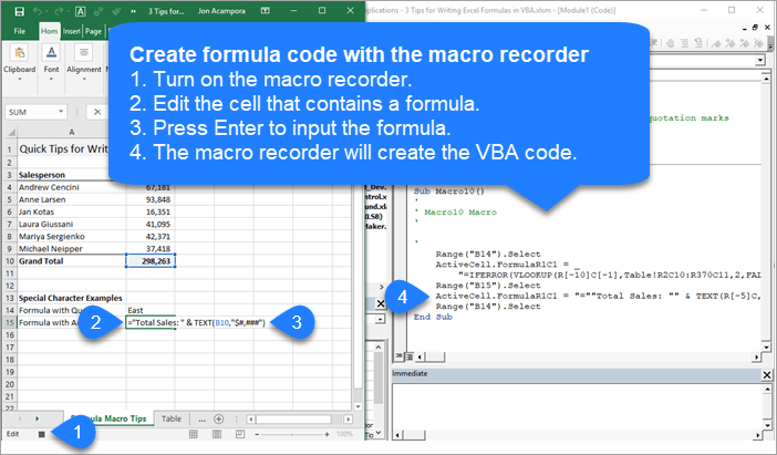
Here are the steps to creating the formula property code with the macro recorder.
- Turn on the macro recorder (Developer tab > Record Macro)
- Type your formula or edit an existing formula.
- Press Enter to enter the formula.
- The code is created in the macro.
If your formula contains quotation marks or ampersand symbols, the macro recorder will account for this. It creates all the sub-strings and wraps everything in quotes properly. Here is an example.
Sub Macro10()
'Use the macro recorder to create code for complex formulas with
'special characters and relative references

  ActiveCell.FormulaR1C1 = "=""Total Sales: "" & TEXT(R[-5]C,""$#,###"")"

End Sub
Tip #3: R1C1 Style Formula Notation
If you use the macro recorder for formulas, you will notices that it creates code with the FormulaR1C1 property.
R1C1 style notation allows us to create both relative (A1), absolute ($A$1), and mixed ($A1, A$1) references in our macro code.
R1C1 stands for Rows and Columns.
Relative References
For relative references we specify the number of rows and columns we want to offset from the cell that the formula is in. The number of rows and columns are referenced in square brackets.
The following would create a reference to a cell that is 3 rows above and 2 rows to the right of the cell that contains the formula.
R[-3]C[2]
Negative numbers go up rows and columns to the left.
Positive numbers go down rows and columns to the right.
Absolute References
We can also use R1C1 notation for absolute references. This would typically look like $A$2.
For absolute references we do NOT use the square brackets. The following would create a direct reference to cell $A$2, row 2 column 1
R2C1
Mixed References
with mixed references we add the square brackets for either the row or column reference, and no brackets for the other reference. The following formula in cell B2 would create this reference to A$2, where the row is absolute and the column is relative.
R2C[-1]
When creating mixed references, the relative row or column number will depend on what cell the formula is in.
It’s easiest to just use the macro recorder to figure these out.
FormulaR1C1 Property versus Formula Property
The FormulaR1C1 property reads the R1C1 notation and creates the proper references in the cells. If you use the regular Formula property with R1C1 notation, then VBA will attempt to put those letters in the formula, and it will likely result in a formula error.
Therefore, use the Formula property when your code contains cell references ($A$1), the FormulaR1C1 property when you need relative references that are applied to multiple cells or dependent on where the formula is entered.
If your spreadsheet changes based on conditions outside your control, like new columns or rows of data are imported from the data source, then relative references and R1C1 style notation will probably be best.
I hope those tips help. Please leave a comment below with questions or suggestions.
|
Дмитрий  Пользователь Сообщений: 11 |
Здравствуйте уважаемые форумчане. Результат представлял себе примерно как-то так, но только, чтобы работало)): ActiveCell.Formula = «=IFERROR(IF((Cells(1,1))*(Cells(1,2))*(Cells(1,lcol))=0,0,1),0)» Запрос продиктован тем, что последний множитель формулы будет находится в последнем столбце таблицы, которая будет ежедневно меняться. *lcol = Cells(1, Columns.Count).End(xlToLeft).Column Заранее благодарю. |
|
Ігор Гончаренко Пользователь Сообщений: 13746 |
#2 28.06.2022 12:54:52
Программисты — это люди, решающие проблемы, о существовании которых Вы не подозревали, методами, которых Вы не понимаете! |
||
|
Дмитрий Пользователь Сообщений: 11 |
Игорь, к сожалению не получается(( Чтобы получить в итоге что-то типо: «=IFERROR(IF((Cells(1,1))*(Cells(1,2))*(Cells(1,lcol))=0,0,1),0)» ? Извиняюсь, все работает — неправильно подтянул ссылку на ячейки в итоговом файл. Изменено: Дмитрий — 28.06.2022 13:35:55 |
|
Дмитрий Пользователь Сообщений: 11 |
Тем не менее вопрос актуален — в макросах вообще возможно написание формул через Cells? |
|
дело не в том, что можно написать в макросе, а дело в том воспримет-ли Excel как корректную формулу, тот текст, что вы набрали макросом и пытаетесь подсунуть ему как формулу напишите функцию использовать теперь RCAdr(9,7) Программисты — это люди, решающие проблемы, о существовании которых Вы не подозревали, методами, которых Вы не понимаете! |
|
|
_Boroda_  Пользователь Сообщений: 1496 Контакты см. в профиле |
#6 28.06.2022 14:09:23
Не получается что? Приложите файл с неполучалкой Скажи мне, кудесник, любимец ба’гов… |
||
|
Jack Famous  Пользователь Сообщений: 10846 OS: Win 8.1 Корп. x64 | Excel 2016 x64: | Browser: Chrome |
#7 28.06.2022 14:47:37
напрямую никак Изменено: Jack Famous — 28.06.2022 14:49:00 Во всех делах очень полезно периодически ставить знак вопроса к тому, что вы с давних пор считали не требующим доказательств (Бертран Рассел) ►Благодарности сюда◄ |
||
|
Ігор Гончаренко Пользователь Сообщений: 13746 |
#8 28.06.2022 15:06:55
при наличии переводчика — вполне))
выполните Test
смотрите в окне Immediate как ReplaceCells преобразовала вашу запись с Cellsами в R1C1 формулу Изменено: Ігор Гончаренко — 28.06.2022 15:08:25 Программисты — это люди, решающие проблемы, о существовании которых Вы не подозревали, методами, которых Вы не понимаете! |
||||||
|
Дмитрий Пользователь Сообщений: 11 |
Большое всем спасибо. Игорь, как написал раньше — самый первый Ваш ответ мне очень помог и исправил мой файл. Насчет обходного пути с написанием функции — буду пробовать. Касательно переводчика — для меня это пока высокая материя, честно — вообще не понимаю код и как он работает, нужно разбираться… Еще раз БОЛЬШОЕ спасибо! |
|
Ігор Гончаренко Пользователь Сообщений: 13746 |
#10 28.06.2022 15:33:35 в коде не обязательно разбираться, достаточно понять как им пользоваться относительно вашего первого поста все может выглядеть так:
при этом не важно поняли вы как работает ReplaceCells или нет, главное — она впихнула в активную ячейку нужную формулу правильно преобразовав ваши Cells в R1C1 адреса ячеек Изменено: Ігор Гончаренко — 28.06.2022 15:38:33 Программисты — это люди, решающие проблемы, о существовании которых Вы не подозревали, методами, которых Вы не понимаете! |
||
|
Hugo Пользователь Сообщений: 23249 |
#11 28.06.2022 16:54:36
— можно использовать адрес ячейки с cells.
|
||||
|
Jack Famous Пользователь Сообщений: 10846 OS: Win 8.1 Корп. x64 | Excel 2016 x64: | Browser: Chrome |
#12 28.06.2022 17:37:08 Hugo, в таком случае нужно обязательно указывать параметры Address и/или принудительно использовать FormulaLocal/FormulaR1C1 Ну и ReplaceCells быстрее будет, т.к. работает с координатами напрямую, а можно ещё ускорить, заменив регулярки строковыми Изменено: Jack Famous — 28.06.2022 17:39:00 Во всех делах очень полезно периодически ставить знак вопроса к тому, что вы с давних пор считали не требующим доказательств (Бертран Рассел) ►Благодарности сюда◄ |
The formulas in Excel, used through VBA are not easy. You need to write a string like "=IFERROR(OR((1=A1),(2=A2)),""No Error"",""Error"")" and this is really not easy and fun to debug. Furthermore, if it is false, VBA will nicely throw a runtime error 1004 and you would start questioning yourself why have you started to program with VBA and you did not continue working as a translator from Greek to Bulgarian (for example).
![]()
And while translating to Greek can be sometimes fun, VBA programming is one step funnier. So, when you are using the formulas in Excel in VBA, you should be aware of the following 3 points:
-
- Each language, which supports Excel has a different formula separator – for German it is “;“, for English it is “,“.
- When you put inverted commas in a formula, you should always escape them with one more inverted commas. Thus, to write
test""you shouldDebug.Print "test""""". 5 times! - There are 4 types of formulas in Excel:
.Formula.FormulaR1C1.FormulaLocal.FormulaR1C1Local
What all these do? Two of them show the formula in the Local language and the other two show it in the R1C1 format.
What is the local language?
If you have ever opened a German Excel, you would have somehow noticed, that the =IF() formula does not exist. There is something called =WENN(). And the same is with about 99% of the formulas. Fortunately, Excel is wise enough that if you send a German Excel with German formulas to an English user, the English user will open the Excel and will see the formulas in his own language. However, VBA generated formulas are not that kind. Thus, if you use .Formula = "=WENN(A1=1;""WAHR"";""FALSCH"") then you will see an error.
If you want to use the language specific formulas, you should use .FormulaLocal = "=WENN(A1=1;""WAHR"";""FALSCH"") as .Formula works only with the English formulas.
What is R1C1 Format?
Excel supports two types of referring to a cell range. The standard with a combination of the alpha column and the row number (A1, B2, C3, etc) and another one, called R1C1. There you give a reference to the row and the column. Thus, A1 is R1C1, B2 is R2C2, C3 is R3C3. So, .FormulaR1C1 = "=IF(R1C1 = 1,""WAHR"",""FALSCH"") would be a valid syntax.
How can you make your life easier?
In general, this is a simple algorithm to follow, which would always help you with the Excel formulas:
- Write the formula, so it works in Excel;
- Select it manually;
- Run the code below;
- It prints the formula as it should look like in the immediate window;
- Copy it & use it;
|
Public Sub PrintMeUsefulFormula() Dim selectedFormula As String Dim parenthesis As String parenthesis = «»«» selectedFormula = Selection.Formula selectedFormula = Replace(selectedFormula, «»«», «»«»«») selectedFormula = parenthesis & selectedFormula & parenthesis Debug.Print selectedFormula End Sub |
Based on which type of formula you have selected, you would see the corresponding result:
-
- .Formula
"=IF(B1=C1,""Equal"",""Not equal"")"
- .FormulaR1C1
"=IF(RC[1]=RC[2],""Equal"",""Not equal"")"
- .FormulaLocal
"=WENN(B1=C1,""Equal"",""Not equal"")"
- .FormulaR1c1Local
-
"=WENN(ZS(1)=ZS(2),""Equal"",""Not equal"")"
-
- .Formula
Once you start using it, you will never go back to writing formulas and contactenating strings manually!
Enjoy it! 🙂
In this lesson you can learn how to add a formula to a cell using vba. There are several ways to insert formulas to cells automatically. We can use properties like Formula, Value and FormulaR1C1 of the Range object. This post explains five different ways to add formulas to cells.
Table of contents
How to add formula to cell using VBA
Add formula to cell and fill down using VBA
Add sum formula to cell using VBA
How to add If formula to cell using VBA
Add formula to cell with quotes using VBA
Add Vlookup formula to cell using VBA
We use formulas to calculate various things in Excel. Sometimes you may need to enter the same formula to hundreds or thousands of rows or columns only changing the row numbers or columns. For an example let’s consider this sample Excel sheet.
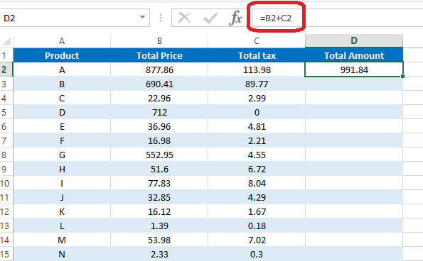
In this Excel sheet I have added a very simple formula to the D2 cell.
=B2+C2
So what if we want to add similar formulas for all the rows in column D. So the D3 cell will have the formula as =B3+C3 and D4 will have the formula as =B4+D4 and so on. Luckily we don’t need to type the formulas manually in all rows. There is a much easier way to do this. First select the cell containing the formula. Then take the cursor to the bottom right corner of the cell. Mouse pointer will change to a + sign. Then left click and drag the mouse until the end of the rows.
However if you want to add the same formula again and again for lots of Excel sheets then you can use a VBA macro to speed up the process. First let’s look at how to add a formula to one cell using vba.
How to add formula to cell using VBA
Lets see how we can enter above simple formula(=B2+C2) to cell D2 using VBA
In this method we are going to use the Formula property of the Range object.
Sub AddFormula_Method1()
Dim WS As Worksheet
Set WS = Worksheets(«Sheet1»)
WS.Range(«D2»).Formula = «=B2+C2»
End Sub
We can also use the Value property of the Range object to add a formula to a cell.
Sub AddFormula_Method2()
Dim WS As Worksheet
Set WS = Worksheets(«Sheet1»)
WS.Range(«D2»).Value = «=B2+C2»
End Sub
Next method is to use the FormulaR1C1 property of the Range object. There are few different ways to use FormulaR1C1 property. We can use absolute reference, relative reference or use both types of references inside the same formula.
In the absolute reference method cells are referred to using numbers. Excel sheets have numbers for each row. So you should think similarly for columns. So column A is number 1. Column B is number 2 etc. Then when writing the formula use R before the row number and C before the column number. So the cell A1 is referred to by R1C1. A2 is referred to by R2C1. B3 is referred to by R3C2 etc.
This is how you can use the absolute reference.
Sub AddFormula_Method3A()
Dim WS As Worksheet
Set WS = Worksheets(«Sheet1»)
WS.Range(«D2»).FormulaR1C1 = «=R2C2+R2C3»
End Sub
If you use the absolute reference, the formula will be added like this.
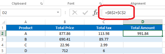
If you use the manual drag method explained above to fill down other rows, then the same formula will be copied to all the rows.
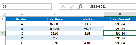
In Majority cases this is not how you want to fill down the formula. However this won’t happen in the relative method. In the relative method, cells are given numbers relative to the cell where the formula is entered. You should use negative numbers when referring to the cells in upward direction or left. Also the numbers should be placed within the square brackets. And you can omit [0] when referring to cells on the same row or column. So you can use RC[-2] instead of R[0]C[-2]. The macro recorder also generates relative reference type code, if you enter a formula to a cell while enabling the macro recorder.
Below example shows how to put formula =B2+C2 in D2 cell using relative reference method.
Sub AddFormula_Method3B()
Dim WS As Worksheet
Set WS = Worksheets(«Sheet1»)
WS.Range(«D2»).FormulaR1C1 = «=RC[-2]+RC[-1]»
End Sub
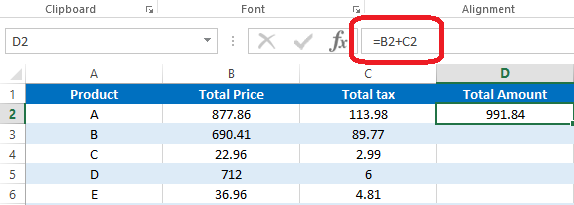
Now use the drag method to fill down all the rows.
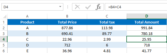
You can see that the formulas are changed according to the row numbers.
Also you can use both relative and absolute references in the same formula. Here is a typical example where you need a formula with both reference types.
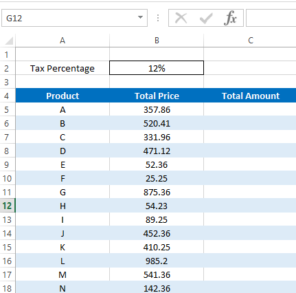
We can add the formula to calculate Total Amount like this.
Sub AddFormula_Method3C()
Dim WS As Worksheet
Set WS = Worksheets(«Sheet2»)
WS.Range(«C5»).FormulaR1C1 = «=RC[-1]+RC[-1]*R2C2»
End Sub
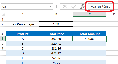
In this formula we have a absolute reference after the * symbol. So when we fill down the formula using the drag method that part will remain the same for all the rows. Hence we will get correct results for all the rows.
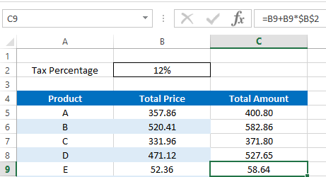
Add formula to cell and fill down using VBA
So now you’ve learnt various methods to add a formula to a cell. Next let’s look at how to fill down the other rows with the added formula using VBA.
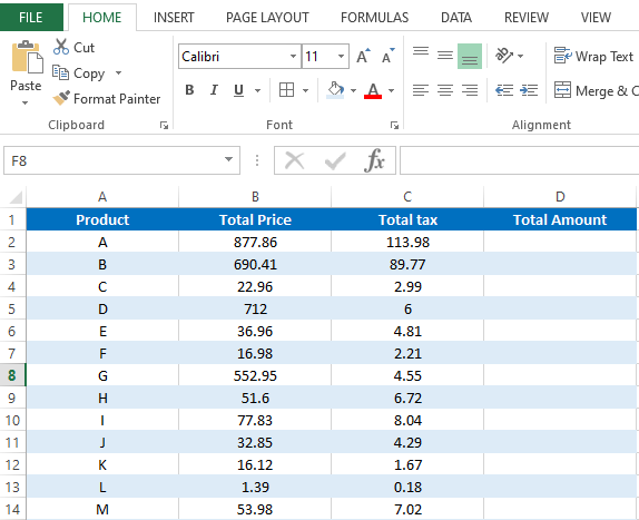
Assume we have to calculate cell D2 value using =B2+C2 formula and fill down up to 1000 rows. First let’s see how we can modify the first method to do this. Let’s name this subroutine as “AddFormula_Method1_1000Rows”
Sub AddFormula_Method1_1000Rows()
End Sub
Then we need an additional variable for the For Next statement
Dim WS As Worksheet
Dim i As Integer
Next, assign the worksheet to WS variable
Set WS = Worksheets(«Sheet1»)
Now we can add the For Next statement like this.
For i = 2 To 1000
WS.Range(«D» & i).Formula = «=B» & i & «+C» & i
Next i
Here I have used «D» & i instead of D2 and «=B» & i & «+C» & i instead of «=B2+C2». So the formula keeps changing like =B3+C3, =B4+C4, =B5+C5 etc. when iterated through the For Next loop.
Below is the full code of the subroutine.
Sub AddFormula_Method1_1000Rows()
Dim WS As Worksheet
Dim i As Integer
Set WS = Worksheets(«Sheet1»)
For i = 2 To 1000
WS.Range(«D» & i).Formula = «=B» & i & «+C» & i
Next i
End Sub
So that’s how you can use VBA to add formulas to cells with variables.
Next example shows how to modify the absolute reference type of FormulaR1C1 method to add formulas upto 1000 rows.
Sub AddFormula_Method3A_1000Rows()
Dim WS As Worksheet
Dim i As Integer
Set WS = Worksheets(«Sheet1»)
For i = 2 To 1000
WS.Range(«D» & i).FormulaR1C1 = «=R» & i & «C2+R» & i & «C3»
Next i
End Sub
You don’t need to do any change to the formula section when modifying the relative reference type of the FormulaR1C1 method.
Sub AddFormula_Method3B_1000Rows()
Dim WS As Worksheet
Dim i As Integer
Set WS = Worksheets(«Sheet1»)
For i = 2 To 1000
WS.Range(«D» & i).FormulaR1C1 = «=RC[-2]+RC[-1]»
Next i
End Sub
Use similar techniques to modify other two types of subroutines to add formulas for multiple rows. Now you know how to add formulas to cells with a variable. Next let’s look at how to add formulas with some inbuilt functions using VBA.
How to add sum formula to a cell using VBA
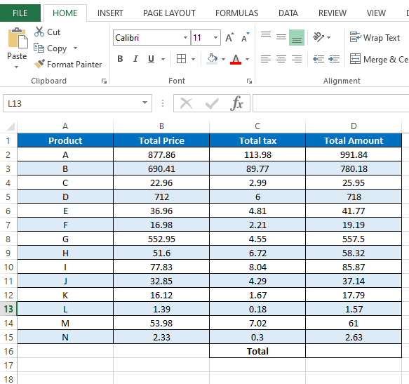
Suppose we want the total of column D in the D16 cell. So this is the formula we need to create.
=SUM(D2:D15)
Now let’s see how to add this using VBA. Let’s name this subroutine as SumFormula.
First let’s declare a few variables.
Dim WS As Worksheet
Dim StartingRow As Long
Dim EndingRow As Long
Assign the worksheet to the variable.
Set WS = Worksheets(«Sheet3»)
Assign the starting row and the ending row to relevant variables.
StartingRow = 2
EndingRow = 1
Then the final step is to create the formula with the above variables.
WS.Range(«D16»).Formula = «=SUM(D» & StartingRow & «:D» & EndingRow & «)»
Below is the full code to add the Sum formula using VBA.
Sub SumFormula()
Dim WS As Worksheet
Dim StartingRow As Long
Dim EndingRow As Long
Set WS = Worksheets(«Sheet3»)
StartingRow = 2
EndingRow = 15
WS.Range(«D16»).Formula = «=SUM(D» & StartingRow & «:D» & EndingRow & «)»
End Sub
How to add If Formula to a cell using VBA
If function is a very popular inbuilt worksheet function available in Microsoft Excel. This function has 3 arguments. Two of them are optional.
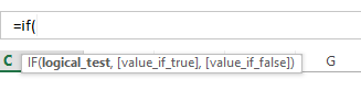
Now let’s see how to add a If formula to a cell using VBA. Here is a typical example where we need a simple If function.
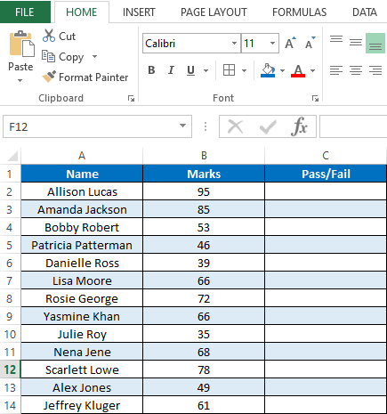
This is the results of students on an examination. Here we have names of students in column A and their marks in column B. Students should get “Pass” if he/she has marks equal or higher than 40. If marks are less than 40 then Excel should show the “Fail” in column C. We can simply obtain this result by adding an If function to column C. Below is the function we need in the C2 cell.
=IF(B2>=40,»Pass»,»Fail»)
Now let’s look at how to add this If Formula to a C2 cell using VBA. Once you know how to add it then you can use the For Next statement to fill the rest of the rows like we did above. We discussed a few different ways to add formulas to a range object using VBA. For this particular example I’m going to use the Formula property of the Range object.
So now let’s see how we can develop this macro. Let’s name this subroutine as “AddIfFormula”
Sub AddIfFormula()
End Sub
However we can’t simply add this If formula using the Formula property like we did before. Because this If formula has quotes inside it. So if we try to add the formula to the cell with quotes, then we get a syntax error.
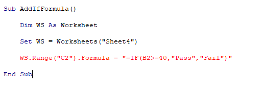
Add formula to cell with quotes
There are two ways to add the formula to a cell with quotes.
Sub AddIfFormula_Method1()
Dim WS As Worksheet
Set WS = Worksheets(«Sheet4»)
WS.Range(«C2»).Formula = «=IF(B2>=40,»»Pass»»,»»Fail»»)»
End Sub
Sub AddIfFormula_Method2()
Dim WS As Worksheet
Set WS = Worksheets(«Sheet4»)
WS.Range(«C2»).Formula = «=IF(B2>=40,» & Chr(34) & «Pass» & Chr(34) & «,» & Chr(34) & «Fail» & Chr(34) & «)»
End Sub
Add vlookup formula to cell using VBA
Finally I will show you how to add a vlookup formula to a cell using VBA. So I created a very simple example where we can use a Vlookup function. Assume we have this section in the Sheet5 of the same workbook.
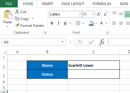
So here when we change the name of the student in the C2 cell, his/her pass or fail status should automatically be shown in the C3 cell. If the original data(data we used in the above “If formula” example) is listed in the Sheet4 then we can write a Vlookup formula for the C3 cell like this.
=VLOOKUP(Sheet5!C2,Sheet4!A2:C200,3,FALSE)
We can use the Formula property of the Range object to add this Vlookup formula to the C3 using VBA.
Sub AddVlookupFormula()
Dim WS As Worksheet
Set WS = Worksheets(«Sheet5»)
WS.Range(«C3»).Formula = «=VLOOKUP(Sheet5!C2,Sheet4!A2:C200,3,FALSE)»
End Sub