
Содержание
- Excel VBA How to Filter Data Using AutoFilter
- CLICK HERE TO GET 5 FREE EXCEL TEMPLATES
- Filter on a Single Criteria
- Filter on Two “Or” Criteria
- Filter on More Than Two “Or” Criteria Using Array
- Filter on Two “And” Criteria
- Filter on Top/Bottom X Values
- Perform Dynamic Date Filters
- Perform Dynamic Average Filters
- Perform a Filter Based on Cell Colour
- Perform a Filter Based on Icon
- Perform Wildcard Filters on Text Fields
- ON-SITE OR ONLINE TRAINING
- 0800 612 4105
- info@bluepecan.co.uk
- Суперфильтр на VBA
- Шаг 1. Именованный диапазон для условий
- Шаг 2. Добавляем макрос фильтрации
- VBA Excel. Функция Filter (фильтрация массива)
- Функция Filter
- Примечания
- Синтаксис
- Параметры
- Compare (значения)
- Пример фильтрации
- filter out multiple criteria using excel vba
- 8 Answers 8
- Excel vba filter and or
Excel VBA How to Filter Data Using AutoFilter
Use the AutoFilter method to perform filters on data
CLICK HERE TO GET 5 FREE EXCEL TEMPLATES
Code examples relate to this database.

Filter on a Single Criteria
This code would filter the data so that only cash payments were displayed.
Filter on Two “Or” Criteria
Use the xlOr operator to perform “Or” criteria.
Filter on More Than Two “Or” Criteria Using Array
NB You have to use the xlFilterValues operator when using an Array as your criteria.
Filter on Two “And” Criteria
Use the xlAnd operator to perform “And” criteria.
Filter on Top/Bottom X Values
Use the Criteria parameter to specify the number of records to return.
Perform Dynamic Date Filters
Excel’s Autofilter allows you to apply date filters that for example filter for dates in the current month, quarter or year, as well as filters for past and future periods. These can be accessed in VBA. You will need to use xlFilterDynamic as your Operator. The following code filters the date field for dates in the current month. Use CTRL SPACE to open the IntelliSense list which includes all the dynamic filter names.
Perform Dynamic Average Filters
This code filters the TRANS_VALUE column for the above average values.
Perform a Filter Based on Cell Colour
Perform a Filter Based on Icon
This code filters for cells containing a red traffic light.
Perform Wildcard Filters on Text Fields
You can use the * and ? wildcard characters in the usual way.
To apply filters to more than one field, you could do this…

ON-SITE OR ONLINE TRAINING
0800 612 4105
info@bluepecan.co.uk
Visitors from YouTube, please click here before you contact us.
Источник
Суперфильтр на VBA
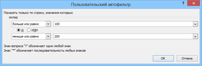
Стандартный Автофильтр для выборки из списков — вещь, безусловно, привычная и надежная. Но для создания сложных условий приходится выполнить не так уж мало действий. Например, чтобы отфильтровать значения попадающие в интервал от 100 до 200, необходимо развернуть список Автофильтра мышью, выбрать вариант Условие (Custom) , а в новых версиях Excel: Числовые фильтры — Настраиваемый фильтр (Number filters — Custom filter) . Затем в диалоговом окне задать два оператора сравнения, значения и логическую связку (И-ИЛИ) между ними:
Не так уж и долго, скажут некоторые. Да, но если в день приходится повторять эту процедуру по нескольку десятков раз? Выход есть — альтернативный фильтр с помощью макроса, который будет брать значения критериев отбора прямо из ячеек листа, куда мы их просто введем с клавиатуры. По сути, это будет похоже на расширенный фильтр, но работающий в реальном времени. Чтобы реализовать такую штуку, нам потребуется сделать всего два шага:
Шаг 1. Именованный диапазон для условий
Сначала надо создать именованный диапазон, куда мы будем вводить условия, и откуда макрос их будет брать. Для этого можно прямо над таблицей вставить пару-тройку пустых строк, затем выделить ячейки для будущих критериев (на рисунке это A2:F2) и дать им имя Условия, вписав его в поле имени в левом верхнем углу и нажав клавишу Enter. Для наглядности, я выделил эти ячейки желтым цветом:
Шаг 2. Добавляем макрос фильтрации
Теперь надо добавить к текущему листу макрос фильтрации по критериям из созданного диапазона Условия. Для этого щелкните правой кнопкой мыши по ярлычку листа и выберите команду Исходный текст (Source text) . В открывшееся окно редактора Visual Basic надо скопировать и вставить текст вот такого макроса:
Теперь при вводе любых условий в желтые ячейки нашего именованного диапазона тут же будет срабатывать фильтрация, отображая только нужные нам строки и скрывая ненужные:
Как и в случае с классическими Автофильтром (Filter) и Расширенным фильтром (Advanced Filter) , в нашем фильтре макросом можно смело использовать символы подстановки:
- * (звездочка) — заменяет любое количество любых символов
- ? (вопросительный знак) — заменяет один любой символ
и операторы логической связки:
- И — выполнение обоих условий
- ИЛИ — выполнение хотя бы одного из двух условий
и любые математические символы неравенства (>, =, ).
При удалении содержимого ячеек желтого диапазона Условия автоматически снимается фильтрация с соответствующих столбцов.
Источник
VBA Excel. Функция Filter (фильтрация массива)
Фильтрация одномерного массива в VBA Excel с помощью функции Filter. Синтаксис и параметры функции Filter. Пример фильтрации одномерного массива.
Функция Filter
Примечания
- исходный (фильтруемый) массив должен быть одномерным и содержать строки;
- индексация возвращенного массива начинается с нуля;
- возвращенный массив содержит ровно столько элементов, сколько строк исходного массива соответствуют заданным условиям фильтрации;
- переменная, которой присваивается возвращенный массив, должна быть универсального типа (As Variant) и объявлена не как массив (не myArray() со скобками, а myArray без скобок).
Функция Filter автоматически преобразует обычную переменную универсального типа, которой присваивается отфильтрованный список, в одномерный массив с необходимым количеством элементов.
Синтаксис
Параметры
| Параметр | Описание |
|---|---|
| sourcearray | Обязательный параметр. Одномерный массив, элементы которого требуется отфильтровать |
| match | Обязательный параметр. Искомая строка. |
| include | Необязательный параметр. Значение Boolean, которое указывает:
|
| compare | Необязательный параметр. Числовое значение (константа), указывающее тип сравнения строк. По умолчанию – 0 (vbBinaryCompare). |
Compare (значения)
Параметр compare может принимать следующие значения:
| Константа | Значение | Описание |
|---|---|---|
| vbUseCompareOption | -1 | используется тип сравнения, заданный оператором Option Compare |
| vbBinaryCompare | 0 | выполняется двоичное сравнение (регистр имеет значение) |
| vbTextCompare | 1 | выполняется текстовое сравнение (без учета регистра) |
Пример фильтрации
Фильтрация списка в столбце «A» по словам, начинающимся с буквы «К», и загрузка результатов в столбец «B»:
Источник
filter out multiple criteria using excel vba
I have 8 variables in column A, 1,2,3,4,5 and A, B, C.
My aim is to filter out A, B, C and display only 1-5.
I can do this using the following code:
But what the code does is it filters variables 1 to 5 and displays them.
I want to do the opposite, but yielding the same result, by filtering out A, B, C and showing variables 1 to 5
I tried this code:
But it did not work.
Why cant I use this code ?
It gives this error:
Run time error 1004 autofilter method of range class failed
How can I perform this?
8 Answers 8
I think (from experimenting — MSDN is unhelpful here) that there is no direct way of doing this. Setting Criteria1 to an Array is equivalent to using the tick boxes in the dropdown — as you say it will only filter a list based on items that match one of those in the array.
Interestingly, if you have the literal values «<>A» and «<>B» in the list and filter on these the macro recorder comes up with
which works. But if you then have the literal value «<>C» as well and you filter for all three (using tick boxes) while recording a macro, the macro recorder replicates precisely your code which then fails with an error. I guess I’d call that a bug — there are filters you can do using the UI which you can’t do with VBA.
Anyway, back to your problem. It is possible to filter values not equal to some criteria, but only up to two values which doesn’t work for you:
There are a couple of workarounds possible depending on the exact problem:
Источник
Excel vba filter and or
The other day I was flipping back and forth between two tables with related sets of data and comparing the rows for one person in each set. I do this kind of thing all the time and often end up filtering each table to the same person, location, date, or whatever, in order to compare their rows more easily. I thought “Wouldn’t it be great to write a little utility that filters a field in one table based on the same criteria as a filter in another table?” Like many questions that begin with “Wouldn’t it be great to write a little utility” this one led me on a voyage of discovery. The utility isn’t finished, but I know a lot more about Autofilter VBA operator parameters.
My biggest discovery is that the parameters used in the Range.Autofilter method to set a filter don’t always match the properties of the Filter object used to read the criteria. For instance, you filter on a cell’s color by passing its RGB value to Criteria1. But when reading the RGB value of a Filter object, Criteria1 suddenly has a Color property. More about this and some other such wrinkles as we go along.
I also realized there are a bunch of xlDynamicFilter settings – like averages and dates – that all use the same operator and are specified by setting the Criteria1 argument.
I also noticed a typo in the xlFilterAllDatesInPeriodFebruray operator. I wonder if anybody has ever even used it?
The Basics – Setting a Filter in VBA
To review the basics of setting Autofilters in VBA you can peruse the skimpy help page. To add a bit to that, let’s return to one of my favorite tables:

Its columns have several characteristices on which you can filter, including text, dates and colors. Here it’s filtered to names that contain “A”, pies with the word “Berry”, dates in the current month and puke-green:

To filter the pies to just berry you have to load their names into an array and set Criteria1 and Operator like:
Sub PieTableFilters()
Dim lo As Excel.ListObject
Dim BerryPies As Variant
Set lo = ActiveWorkbook.Worksheets( «pie orders» ).ListObjects(1)
BerryPies = Array( «Strawberry» , «Blueberry» , «Razzleberry» , «Boysenberry» )
lo.DataBodyRange.AutoFilter field:=2, _
Criteria1:=BerryPies, Operator:=xlFilterValues
End Sub
Discovery #1 – An xlFilterValues Array Set With Two Values Becomes an xlOR Operator:
To read the filter created by the code above, I’d still use the xlFilterValues operator and read the array from Criteria1. However, if the column was filtered to only two types of pies, I’d use the xlOR operator and Criteria1 and Criteria2. This is unchanged since Johh Walkenbach posted about Stephen Bullen’s function to read filters settings for Excel 2003.
Similarly, if I set a filter with a one-element array, e.g., only one type of pie, and then read the filter operator it returns a 0.
The Basics, Continued – Setting a Color Filter
Here’s how to set the filter for the last column. It’s based on cell color. Note that it works for Conditional Formatting colors as well as regular fill colors:
Here 8643294 is the RGB value of that greenish color. In order to determine that RGB in code, you need to use something like:
Discovery #2 – The Filter.Criteria1 Property Sometimes has Sub-Properties, Like Color:
Note that the RGB isn’t in Criteria1 – it’s in Criteria1.Color, a property I only discovered by digging around in the Locals window:

Also note that there are a bunch of other properties there, like Pattern, etc.
Further, if a column is filtered by conditional formatting icon (yes you can do that) using the xlFilterIcon(10) parameter then Criteria1 contains an Icon property. This property is numbered 1 to 4 (I think) and relates to the position of the icon in its group.
Discovery #3: xlDynamicFilter and Its Many Settings
The xlFilterDynamic operator, enum 11, is a broad category of settings. You narrow them down in Criteria1. So, for instance, you can filter a column to the current month like:
This is a good time to mention the chart below that contains all of these xlDynamicFilter operators and their enums. Looking at it you’ll note that in addition to a whole lot of date filters (all of which appear in Excel’s front end as well) there’s also the Above Average and Below Average filters.
Discovery #4: Top 10 Settings Are Weird
To set a Top 10 item in VBA you do something like this:
Here, I’ve actually filtered column 4 to the top three items (As stated in Help, Criteria1 contains the actual number of items to filter). If I look at the filter settings for that column in the table I’ll see that Number Filters is checked and the dialog shows “Top 10.” That makes sense.
However if we look at the locals window right after the line above is executed, we see that the number 3 which we coded in Criteria1 is replaced by a greater than formula:

Further, if I then wanted to apply this filter to another column based only on what I’m able to read in VBA, I’d have to change it to:
Note that I don’t use an operator at all. We could also use xlFilterValues or xlOr. Using nothing best reflects what shows in the locals window, where the operator changes to 0 after the code above is executed.
The Chart
Below is a chart, contained in a OneDrive usable and downloadable workbook, that summarizes much of the above. It includes all the possible Autofilter VBA Operator parameters, as well as all the sub-parameters for the xlFilterDynamic operator.
Discovery #5: February is the Hardest Month (to spell)
I like to automate things as much as possible, so generating the list of xlFilterDynamic properties was kind of a pain. To get the list of constants from the Object Browser I had to copy and paste one by one into Excel, where I cobbled together a line of VBA for each one, like:
Debug.Print “xlFilterAboveAverage: ” & xlFilterAboveAverage
Of course I saw I didn’t need to paste all the month operators into Excel since I could just drag “January” down eleven more cells and append the generated month names. Minutes saved!
But when I ran the code it choked on February. It was then I noticed that its constant is misspelled.
Two More Tips
1. Use Enum Numbers, not Constants: This misspelling of February points out a good practice when using any set of enums: use the number, not the constants. For example, use 8, not xlFilterValues. This helps in case the constants are changed in future Excel versions, and with international compatibility, late binding and, at least in this case, spelling errors. Of course it’s not nearly as readable and you have to figure out the enums.
2. The Locals Window is Your Friend: I don’t use the Locals window very much, but in working with these Autofilter settings, it was hugely helpful. It revealed things that I don’t think I’d have figured out any other way.
Conclusion – Building a Utility
Armed with my newfound knowledge, I could come close to building a utility that copies filters from one table to another, or one like the Walkenbach/Bullen filter lister linked at the beginning of this post. In most cases I could just transfer the filter by using the source Operator and Criteria1 (and Criteria2 where applicable)
But as we’ve seen, there’s a couple of filter types where the operator and/or criteria change. The worst of these is a Top 10 filter. My first thought was to count the number of unfiltered cells, but if the column has duplicates, e.g., your top value appears three times, that won’t always be accurate. In addition, other columns could be filtered which could also throw off the count.
Transferring a color scale filter would be even trickier as it’s very possible the same color wouldn’t exist in the second table.
Whew! Long post! Leave a comment if you got this far and let me know what you think.
Источник
It’s pretty straight forward to filter down on specific values in your data with VBA code. You just list out the values in an array like so:
Sub FilterOnValues()
‘PURPOSE: Filter on specific values
‘SOURCE: www.TheSpreadsheetGuru.com
Dim rng As Range
Set rng = ActiveSheet.Range(«B7:D18»)
FilterField = WorksheetFunction.Match(«Country», rng.Rows(1), 0)
‘Turn on filter if not already turned on
If ActiveSheet.AutoFilterMode = False Then rng.AutoFilter
‘Filter Specific Countries
rng.AutoFilter Field:=FilterField, Criteria1:=Array( _
«Russia», «China», «Greece», «France»), Operator:=xlFilterValues
End Sub
But what if you have 100 values you want to filter on? Sometimes it’s more efficient to filter out values because there are fewer excluded items than included. Unfortunately, this functionality is not as straightforward as it should be in VBA.
The only way I know to filter out values with VBA is to use Excel’s spreadsheet-based Advanced Filter functionality. This requires you to set up a small data table on your spreadsheet and read-in the criteria with your VBA code. Let’s look into how you can create this very powerful table and take VBA filtering to the next level!
The Advanced Filter Table Setup
The setup of for an Advanced Filter table is vital to properly filter your data just the way you want. Each heading in your designated table (or range if you choose) must match verbatim to the column headings in your data set. Note that you can repeat column names to apply multiple criteria to a single column in your data (do not use an Excel table if you need to do this since tables must have unique column headings).
AND Filters
Any criteria written in the same row in your filter table is treated as an AND statement. You can make your Advanced Filter table as wide as you need to handle multiple criteria. The below example would handle filtering out 4 country names within the Country column of your data set.
OR Filters
Each new row in your Advanced Filter table designates an OR statement. This can be handy if you want to narrow down your data to include one of a few values. In the below example, the advanced filter range would show and row that contained «Maria», «Russia», «France», or a last name that starts with the letter «T».
Based on the above criteria, you can see below how the table would filter the data. The highlighted words are what the Advanced Filter flagged as data the user wanted to see.
Notice in the Last Name column, that any name that begins with the letter «T» gets flagged. This is because a wildcard symbol was used in the Advanced Filter range. By placing an asterisk (*) after the letter «T», you can filter on words that begin with the characters prior to the asterisk.
How To Use Advanced Filtering With VBA
It is very easy to link up your Advanced Filter range into your VBA code. I recommend using a dynamically named range or a table to store your filtering criteria.
Sub AdvancedFilter()
Dim rng As Range
‘Set variable equal to data set range
Set rng = ActiveSheet.Range(«B8:D19»)
‘Filter out certain values (filter indicators will not appear!)
rng.AdvancedFilter Action:=xlFilterInPlace, CriteriaRange:= _
ActiveSheet.ListObjects(«Table4»).Range, Unique:=True
End Sub
This Is Better Than Writing Criteria Inside Your Code
When I began coding in VBA, I would always write data into my code. It was not until I had to train others to use and modify my automations, that I learned very quickly the power of deriving settings and criteria from a user interface (aka spreadsheet) instead of going in and re-writing the VBA code itself.
For example, it would be much easier to tell a co-worker (let’s call her Susan) who has no experience with VBA coding, how to modify an advanced filter table if sometime down the road a new country needs to be filtered on. Introducing Susan to VBA and overwhelming her with lines of a foreign language would certainly be more difficult to explain, and my confidence that she could modify the VBA on her own would not be very high. Save yourself from future headaches and start storing values and settings in a worksheet instead of in your VBA code.
Learn More With This Example Workbook
I have created a sample workbook with 4 different scenarios for handling different types of filtering needs. I also switch up how the code is written by pulling from spreadsheet ranges and Excel tables. The workbook and its code are completely unlocked so you can dig in and discover how the magic works. Hopefully, you start saving some time and automating the filtering of your data with the techniques featured in this article.
If you would like to get a copy of the Excel file I used throughout this article, feel free to directly download the spreadsheet by clicking the download button below.
About The Author
Hey there! I’m Chris and I run TheSpreadsheetGuru website in my spare time. By day, I’m actually a finance professional who relies on Microsoft Excel quite heavily in the corporate world. I love taking the things I learn in the “real world” and sharing them with everyone here on this site so that you too can become a spreadsheet guru at your company.
Through my years in the corporate world, I’ve been able to pick up on opportunities to make working with Excel better and have built a variety of Excel add-ins, from inserting tickmark symbols to automating copy/pasting from Excel to PowerPoint. If you’d like to keep up to date with the latest Excel news and directly get emailed the most meaningful Excel tips I’ve learned over the years, you can sign up for my free newsletters. I hope I was able to provide you with some value today and I hope to see you back here soon!
— Chris
Founder, TheSpreadsheetGuru.com
Фильтрация одномерного массива в VBA Excel с помощью функции Filter. Синтаксис и параметры функции Filter. Пример фильтрации одномерного массива.
Filter – это функция, которая возвращает массив, содержащий строки исходного одномерного массива, соответствующие заданным условиям фильтрации.
Примечания
- исходный (фильтруемый) массив должен быть одномерным и содержать строки;
- индексация возвращенного массива начинается с нуля;
- возвращенный массив содержит ровно столько элементов, сколько строк исходного массива соответствуют заданным условиям фильтрации;
- переменная, которой присваивается возвращенный массив, должна быть универсального типа (As Variant) и объявлена не как массив (не myArray() со скобками, а myArray без скобок).
Функция Filter автоматически преобразует обычную переменную универсального типа, которой присваивается отфильтрованный список, в одномерный массив с необходимым количеством элементов.
Синтаксис
|
Filter(sourcearray, match, [include], [compare]) |
Параметры
| Параметр | Описание |
|---|---|
| sourcearray | Обязательный параметр. Одномерный массив, элементы которого требуется отфильтровать |
| match | Обязательный параметр. Искомая строка. |
| include | Необязательный параметр. Значение Boolean, которое указывает:
|
| compare | Необязательный параметр. Числовое значение (константа), указывающее тип сравнения строк. По умолчанию – 0 (vbBinaryCompare). |
Compare (значения)
Параметр compare может принимать следующие значения:
| Константа | Значение | Описание |
|---|---|---|
| vbUseCompareOption | -1 | используется тип сравнения, заданный оператором Option Compare |
| vbBinaryCompare | 0 | выполняется двоичное сравнение (регистр имеет значение) |
| vbTextCompare | 1 | выполняется текстовое сравнение (без учета регистра) |
Пример фильтрации
Фильтрация списка в столбце «A» по словам, начинающимся с буквы «К», и загрузка результатов в столбец «B»:

Пример кода VBA Excel с функцией Filter:
|
1 2 3 4 5 6 7 8 9 10 11 12 13 14 15 16 17 |
Sub Primer() Dim arr1, arr2, arr3, i As Long ‘Присваиваем переменной arr1 массив значений столбца A arr1 = Range(«A1:A» & Range(«A1»).End(xlDown).Row) ‘Копируем строки двумерного массива arr1 в одномерный arr2 ReDim arr2(1 To UBound(arr1)) For i = 1 To UBound(arr1) arr2(i) = arr1(i, 1) Next ‘Фильтруем строки массива arr2 по вхождению подстроки «К» ‘и присваиваем отфильтрованные строки переменной arr3 arr3 = Filter(arr2, «К») ‘Копируем строки из массива arr3 в столбец «B» For i = 0 To UBound(arr3) Cells(i + 1, 2) = arr3(i) Next End Sub |

A lot of Excel functionalities are also available to be used in VBA – and the Autofilter method is one such functionality.
If you have a dataset and you want to filter it using a criterion, you can easily do it using the Filter option in the Data ribbon.![]()
And if you want a more advanced version of it, there is an advanced filter in Excel as well.
Then Why Even Use the AutoFilter in VBA?
If you just need to filter data and do some basic stuff, I would recommend stick to the inbuilt Filter functionality that Excel interface offers.
You should use VBA Autofilter when you want to filter the data as a part of your automation (or if it helps you save time by making it faster to filter the data).
For example, suppose you want to quickly filter the data based on a drop-down selection, and then copy this filtered data into a new worksheet.
While this can be done using the inbuilt filter functionality along with some copy-paste, it can take you a lot of time to do this manually.
In such a scenario, using VBA Autofilter can speed things up and save time.
Note: I will cover this example (on filtering data based on a drop-down selection and copying into a new sheet) later in this tutorial.
Excel VBA Autofilter Syntax
Expression. AutoFilter( _Field_ , _Criteria1_ , _Operator_ , _Criteria2_ , _VisibleDropDown_ )
- Expression: This is the range on which you want to apply the auto filter.
- Field: [Optional argument] This is the column number that you want to filter. This is counted from the left in the dataset. So if you want to filter data based on the second column, this value would be 2.
- Criteria1: [Optional argument] This is the criteria based on which you want to filter the dataset.
- Operator: [Optional argument] In case you’re using criteria 2 as well, you can combine these two criteria based on the Operator. The following operators are available for use: xlAnd, xlOr, xlBottom10Items, xlTop10Items, xlBottom10Percent, xlTop10Percent, xlFilterCellColor, xlFilterDynamic, xlFilterFontColor, xlFilterIcon, xlFilterValues
- Criteria2: [Optional argument] This is the second criteria on which you can filter the dataset.
- VisibleDropDown: [Optional argument] You can specify whether you want the filter drop-down icon to appear in the filtered columns or not. This argument can be TRUE or FALSE.
Apart from Expression, all the other arguments are optional.
In case you don’t use any argument, it would simply apply or remove the filter icons to the columns.
Sub FilterRows()
Worksheets("Filter Data").Range("A1").AutoFilter
End Sub
The above code would simply apply the Autofilter method to the columns (or if it’s already applied, it will remove it).
This simply means that if you can not see the filter icons in the column headers, you will start seeing it when this above code is executed, and if you can see it, then it will be removed.
In case you have any filtered data, it will remove the filters and show you the full dataset.
Now let’s see some examples of using Excel VBA Autofilter that will make it’s usage clear.
Example: Filtering Data based on a Text condition
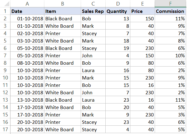
Suppose you have a dataset as shown below and you want to filter it based on the ‘Item’ column.
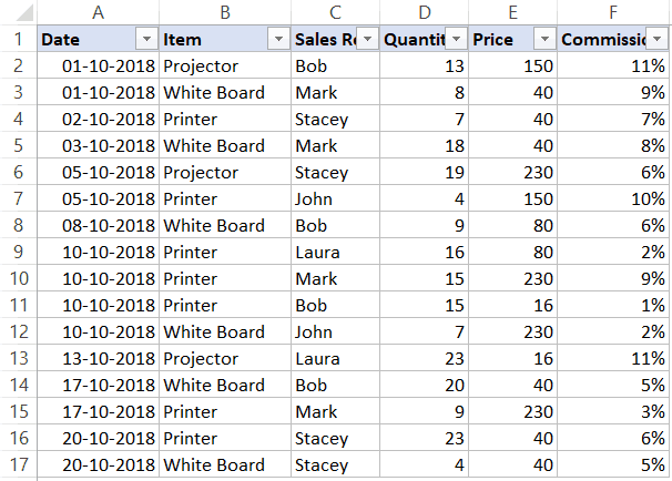
The below code would filter all the rows where the item is ‘Printer’.
Sub FilterRows()
Worksheets("Sheet1").Range("A1").AutoFilter Field:=2, Criteria1:="Printer"
End Sub
The above code refers to Sheet1 and within it, it refers to A1 (which is a cell in the dataset).
Note that here we have used Field:=2, as the item column is the second column in our dataset from the left.
Now if you’re thinking – why do I need to do this using a VBA code. This can easily be done using inbuilt filter functionality.
You’re right!
If this is all you want to do, better used the inbuilt Filter functionality.
But as you read the remaining tutorial, you’ll see that this can be combined with some extra code to create powerful automation.
But before I show you those, let me first cover a few examples to show you what all the AutoFilter method can do.
Click here to download the example file and follow along.
Example: Multiple Criteria (AND/OR) in the Same Column
Suppose I have the same dataset, and this time I want to filter all the records where the item is either ‘Printer’ or ‘Projector’.
The below code would do this:
Sub FilterRowsOR()
Worksheets("Sheet1").Range("A1").AutoFilter Field:=2, Criteria1:="Printer", Operator:=xlOr, Criteria2:="Projector"
End Sub
Note that here I have used the xlOR operator.
This tells VBA to use both the criteria and filter the data if any of the two criteria are met.
Similarly, you can also use the AND criteria.
For example, if you want to filter all the records where the quantity is more than 10 but less than 20, you can use the below code:
Sub FilterRowsAND()
Worksheets("Sheet1").Range("A1").AutoFilter Field:=4, Criteria1:=">10", _
    Operator:=xlAnd, Criteria2:="<20"
End Sub
Example: Multiple Criteria With Different Columns
Suppose you have the following dataset.
With Autofilter, you can filter multiple columns at the same time.
For example, if you want to filter all the records where the item is ‘Printer’ and the Sales Rep is ‘Mark’, you can use the below code:
Sub FilterRows()
With Worksheets("Sheet1").Range("A1")
.AutoFilter field:=2, Criteria1:="Printer"
.AutoFilter field:=3, Criteria1:="Mark"
End With
End Sub
Example: Filter Top 10 Records Using the AutoFilter Method
Suppose you have the below dataset.
Below is the code that will give you the top 10 records (based on the quantity column):
Sub FilterRowsTop10()
ActiveSheet.Range("A1").AutoFilter Field:=4, Criteria1:="10", Operator:=xlTop10Items
End Sub
In the above code, I have used ActiveSheet. You can use the sheet name if you want.
Note that in this example, if you want to get the top 5 items, just change the number in Criteria1:=”10″ from 10 to 5.
So for top 5 items, the code would be:
Sub FilterRowsTop5()
ActiveSheet.Range("A1").AutoFilter Field:=4, Criteria1:="5", Operator:=xlTop10Items
End Sub
It may look weird, but no matter how many top items you want, the Operator value always remains xlTop10Items.
Similarly, the below code would give you the bottom 10 items:
Sub FilterRowsBottom10()
ActiveSheet.Range("A1").AutoFilter Field:=4, Criteria1:="10", Operator:=xlBottom10Items
End Sub
And if you want the bottom 5 items, change the number in Criteria1:=”10″ from 10 to 5.
Example: Filter Top 10 Percent Using the AutoFilter Method
Suppose you have the same data set (as used in the previous examples).
Below is the code that will give you the top 10 percent records (based on the quantity column):
Sub FilterRowsTop10()
ActiveSheet.Range("A1").AutoFilter Field:=4, Criteria1:="10", Operator:=xlTop10Percent
End Sub
In our dataset, since we have 20 records, it will return the top 2 records (which is 10% of the total records).
Example: Using Wildcard Characters in Autofilter
Suppose you have a dataset as shown below:
If you want to filter all the rows where the item name contains the word ‘Board’, you can use the below code:
Sub FilterRowsWildcard()
Worksheets("Sheet1").Range("A1").AutoFilter Field:=2, Criteria1:="*Board*"
End Sub
In the above code, I have used the wildcard character * (asterisk) before and after the word ‘Board’ (which is the criteria).
An asterisk can represent any number of characters. So this would filter any item that has the word ‘board’ in it.
Example: Copy Filtered Rows into a New Sheet
If you want to not only filter the records based on criteria but also copy the filtered rows, you can use the below macro.
It copies the filtered rows, adds a new worksheet, and then pastes these copied rows into the new sheet.
Sub CopyFilteredRows()
Dim rng As Range
Dim ws As Worksheet
If Worksheets("Sheet1").AutoFilterMode = False Then
MsgBox "There are no filtered rows"
Exit Sub
End If
Set rng = Worksheets("Sheet1").AutoFilter.Range
Set ws = Worksheets.Add
rng.Copy Range("A1")
End Sub
The above code would check if there are any filtered rows in Sheet1 or not.
If there are no filtered rows, it will show a message box stating that.
And if there are filtered rows, it will copy those, insert a new worksheet, and paste these rows on that newly inserted worksheet.
Example: Filter Data based on a Cell Value
Using Autofilter in VBA along with a drop-down list, you can create a functionality where as soon as you select an item from the drop-down, all the records for that item are filtered.
Something as shown below:
 Click here to download the example file and follow along.
This type of construct can be useful when you want to quickly filter data and then use it further in your work.
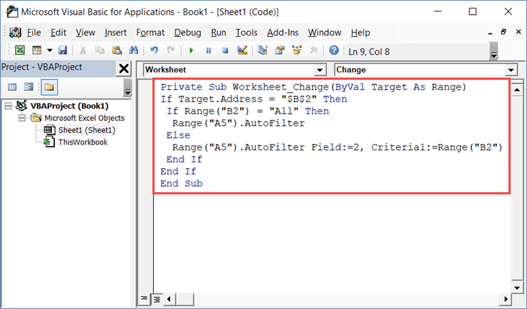
Below is the code that will do this:
Private Sub Worksheet_Change(ByVal Target As Range)
If Target.Address = "$B$2" Then
 If Range("B2") = "All" Then
  Range("A5").AutoFilter
 Else
  Range("A5").AutoFilter Field:=2, Criteria1:=Range("B2")
 End If
End If
End Sub
This is a worksheet event code, which gets executed only when there is a change in the worksheet and the target cell is B2 (where we have the drop-down).
Also, an If Then Else condition is used to check if the user has selected ‘All’ from the drop down. If All is selected, the entire data set is shown.
This code is NOT placed in a module.
Instead, it needs to be placed in the backend of the worksheet that has this data.
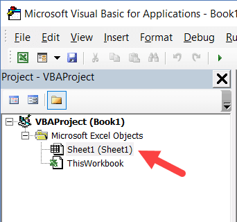
Here are the steps to put this code in the worksheet code window:
- Open the VB Editor (keyboard shortcut – ALT + F11).
- In the Project Explorer pane, double-click on the Worksheet name in which you want this filtering functionality.

- In the worksheet code window, copy and paste the above code.

- Close the VB Editor.
Now when you use the drop-down list, it will automatically filter the data.
This is a worksheet event code, which gets executed only when there is a change in the worksheet and the target cell is B2 (where we have the drop-down).
Also, an If Then Else condition is used to check if the user has selected ‘All’ from the drop down. If All is selected, the entire data set is shown.
Turn Excel AutoFilter ON/OFF using VBA
When applying Autofilter to a range of cells, there may already be some filters in place.
You can use the below code turn off any pre-applied auto filters:
Sub TurnOFFAutoFilter()
  Worksheets("Sheet1").AutoFilterMode = False
End Sub
This code checks the entire sheets and removes any filters that have been applied.
If you don’t want to turn off filters from the entire sheet but only from a specific dataset, use the below code:
Sub TurnOFFAutoFilter()
  If Worksheets("Sheet1").Range("A1").AutoFilter Then
    Worksheets("Sheet1").Range("A1").AutoFilter
  End If
End Sub
The above code checks whether there are already filters in place or not.
If filters are already applied, it removes it, else it does nothing.
Similarly, if you want to turn on AutoFilter, use the below code:
Sub TurnOnAutoFilter()
  If Not Worksheets("Sheet1").Range("A4").AutoFilter Then
    Worksheets("Sheet1").Range("A4").AutoFilter
  End If
End Sub
Check if AutoFilter is Already Applied
If you have a sheet with multiple datasets and you want to make sure you know that there are no filters already in place, you can use the below code.
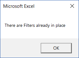
Sub CheckforFilters()
If ActiveSheet.AutoFilterMode = True Then
MsgBox "There are Filters already in place"
Else
MsgBox "There are no filters"
End If
End Sub
This code uses a message box function that displays a message ‘There are Filters already in place’ when it finds filters on the sheet, else it shows ‘There are no filters’.
Show All Data
If you have filters applied to the dataset and you want to show all the data, use the below code:
Sub ShowAllData()
If ActiveSheet.FilterMode Then ActiveSheet.ShowAllData
End Sub
The above code checks whether the FilterMode is TRUE or FALSE.
If it’s true, it means a filter has been applied and it uses the ShowAllData method to show all the data.
Note that this does not remove the filters. The filter icons are still available to be used.
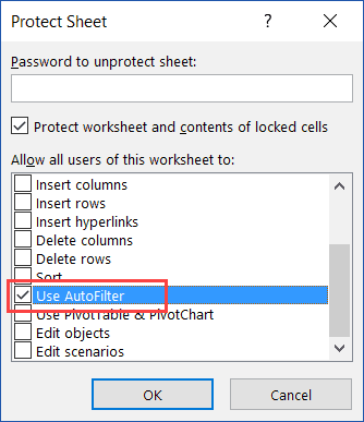
Using AutoFilter on Protected Sheets
By default, when you protect a sheet, the filters won’t work.
In case you already have filters in place, you can enable AutoFilter to make sure it works even on protected sheets.
To do this, check the Use Autofilter option while protecting the sheet.
While this works when you already have filters in place, in case you try to add Autofilters using a VBA code, it won’t work.
Since the sheet is protected, it wouldn’t allow any macro to run and make changes to the Autofilter.
So you need to use a code to protect the worksheet and make sure auto filters are enabled in it.
This can be useful when you have created a dynamic filter (something I covered in the example – ‘Filter Data based on a Cell Value’).
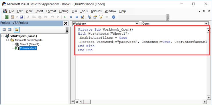
Below is the code that will protect the sheet, but at the same time, allow you to use Filters as well as VBA macros in it.
Private Sub Workbook_Open()
With Worksheets("Sheet1")
.EnableAutoFilter = True
.Protect Password:="password", Contents:=True, UserInterfaceOnly:=True
End With
End Sub
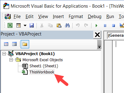
This code needs to be placed in ThisWorkbook code window.
Here are the steps to put the code in ThisWorkbook code window:
- Open the VB Editor (keyboard shortcut – ALT + F11).
- In the Project Explorer pane, double-click on the ThisWorkbook object.

- In the code window that opens, copy and paste the above code.

As soon as you open the workbook and enable macros, it will run the macro automatically and protect Sheet1.
However, before doing that, it will specify ‘EnableAutoFilter = True’, which means that the filters would work in the protected sheet as well.
Also, it sets the ‘UserInterfaceOnly’ argument to ‘True’. This means that while the worksheet is protected, the VBA macros code would continue to work.
You May Also Like the Following VBA Tutorials:
- Excel VBA Loops.
- Filter Cells with Bold Font Formatting.
- Recording a Macro.
- Sort Data Using VBA.
- Sort Worksheet Tabs in Excel.
Стандартный Автофильтр для выборки из списков — вещь, безусловно, привычная и надежная. Но для создания сложных условий приходится выполнить не так уж мало действий. Например, чтобы отфильтровать значения попадающие в интервал от 100 до 200, необходимо развернуть список Автофильтра мышью, выбрать вариант Условие (Custom), а в новых версиях Excel: Числовые фильтры — Настраиваемый фильтр (Number filters — Custom filter). Затем в диалоговом окне задать два оператора сравнения, значения и логическую связку (И-ИЛИ) между ними:
Не так уж и долго, скажут некоторые. Да, но если в день приходится повторять эту процедуру по нескольку десятков раз? Выход есть — альтернативный фильтр с помощью макроса, который будет брать значения критериев отбора прямо из ячеек листа, куда мы их просто введем с клавиатуры. По сути, это будет похоже на расширенный фильтр, но работающий в реальном времени. Чтобы реализовать такую штуку, нам потребуется сделать всего два шага:
Шаг 1. Именованный диапазон для условий
Сначала надо создать именованный диапазон, куда мы будем вводить условия, и откуда макрос их будет брать. Для этого можно прямо над таблицей вставить пару-тройку пустых строк, затем выделить ячейки для будущих критериев (на рисунке это A2:F2) и дать им имя Условия, вписав его в поле имени в левом верхнем углу и нажав клавишу Enter. Для наглядности, я выделил эти ячейки желтым цветом:
Шаг 2. Добавляем макрос фильтрации
Теперь надо добавить к текущему листу макрос фильтрации по критериям из созданного диапазона Условия. Для этого щелкните правой кнопкой мыши по ярлычку листа и выберите команду Исходный текст (Source text). В открывшееся окно редактора Visual Basic надо скопировать и вставить текст вот такого макроса:
Private Sub Worksheet_Change(ByVal Target As Range)

    Dim FilterCol As Integer
    Dim FilterRange As Range
    Dim CondtitionString As Variant
    Dim Condition1 As String, Condition2 As String

    If Intersect(Target, Range("Условия")) Is Nothing Then Exit Sub

    On Error Resume Next
    Application.ScreenUpdating = False

    'определяем диапазон данных списка
    Set FilterRange = Target.Parent.AutoFilter.Range

    'считываем условия из всех измененных ячеек диапазона условий
    For Each cell In Target.Cells
        FilterCol = cell.Column - FilterRange.Columns(1).Column + 1

        If IsEmpty(cell) Then
            Target.Parent.Range(FilterRange.Address).AutoFilter Field:=FilterCol
        Else
            If InStr(1, UCase(cell.Value), " ИЛИ ") > 0 Then
                LogicOperator = xlOr
                ConditionArray = Split(UCase(cell.Value), " ИЛИ ")
            Else
                If InStr(1, UCase(cell.Value), " И ") > 0 Then
                    LogicOperator = xlAnd
                    ConditionArray = Split(UCase(cell.Value), " И ")
                Else
                    ConditionArray = Array(cell.Text)
                End If
            End If
            'формируем первое условие
            If Left(ConditionArray(0), 1) = "<" Or Left(ConditionArray(0), 1) = ">" Then
                Condition1 = ConditionArray(0)
            Else
                Condition1 = "=" & ConditionArray(0)
            End If
            'формируем второе условие - если оно есть
            If UBound(ConditionArray) = 1 Then
                If Left(ConditionArray(1), 1) = "<" Or Left(ConditionArray(1), 1) = ">" Then
                    Condition2 = ConditionArray(1)
                Else
                    Condition2 = "=" & ConditionArray(1)
                End If
            End If
            'включаем фильтрацию
            If UBound(ConditionArray) = 0 Then
                Target.Parent.Range(FilterRange.Address).AutoFilter Field:=FilterCol, Criteria1:=Condition1
            Else
                Target.Parent.Range(FilterRange.Address).AutoFilter Field:=FilterCol, Criteria1:=Condition1, _
                    Operator:=LogicOperator, Criteria2:=Condition2
            End If
        End If
    Next cell

    Set FilterRange = Nothing
    Application.ScreenUpdating = True
End Sub
Все.
Теперь при вводе любых условий в желтые ячейки нашего именованного диапазона тут же будет срабатывать фильтрация, отображая только нужные нам строки и скрывая ненужные:
Как и в случае с классическими Автофильтром (Filter) и Расширенным фильтром (Advanced Filter), в нашем фильтре макросом можно смело использовать символы подстановки:
- * (звездочка) — заменяет любое количество любых символов
- ? (вопросительный знак) — заменяет один любой символ
и операторы логической связки:
- И — выполнение обоих условий
- ИЛИ — выполнение хотя бы одного из двух условий
и любые математические символы неравенства (>,<,=,>=,<=,<>).
При удалении содержимого ячеек желтого диапазона Условия автоматически снимается фильтрация с соответствующих столбцов.
P.S.
- Если у вас Excel 2007 или 2010 не забудьте сохранить файл с поддержкой макросов (в формате xlsm), иначе добавленный макрос умрет.
- Данный макрос не умеет работать с «умными таблицами»
Ссылки по теме
- Что такое макросы, куда вставлять код макроса на VBA, как их использовать?
- Умные таблицы Excel 2007/2010
- Расширенный фильтр и немного магии