Excel vba что такое entirerow

title	keywords	f1_keywords	ms.prod	api_name	ms.assetid	ms.date	ms.localizationpriority
Range.EntireRow property (Excel)	vbaxl10.chm144123	vbaxl10.chm144123	excel	Excel.Range.EntireRow	9e66da51-6cef-4109-ea4e-2acaad42aa1f	05/10/2019	medium

Range.EntireRow property (Excel)

Returns a Range object that represents the entire row (or rows) that contains the specified range. Read-only.

Syntax

expression.EntireRow

expression A variable that represents a Range object.

Example

This example sets the value of the first cell in the row that contains the active cell. The example must be run from a worksheet.

ActiveCell.EntireRow.Cells(1, 1).Value = 5

This example sorts all the rows on a worksheet, including hidden rows.

Sub SortAll()
    'Turn off screen updating, and define your variables.
    Application.ScreenUpdating = False
    Dim lngLastRow As Long, lngRow As Long
    Dim rngHidden As Range
    
    'Determine the number of rows in your sheet, and add the header row to the hidden range variable.
    lngLastRow = Cells(Rows.Count, 1).End(xlUp).Row
    Set rngHidden = Rows(1)
    
    'For each row in the list, if the row is hidden add that row to the hidden range variable.
    For lngRow = 1 To lngLastRow
        If Rows(lngRow).Hidden = True Then
            Set rngHidden = Union(rngHidden, Rows(lngRow))
        End If
    Next lngRow
    
    'Unhide everything in the hidden range variable.
    rngHidden.EntireRow.Hidden = False
    
    'Perform the sort on all the data.
    Range("A1").CurrentRegion.Sort _
        key1:=Range("A2"), _
        order1:=xlAscending, _
        header:=xlYes
        
    'Re-hide the rows that were originally hidden, but unhide the header.
    rngHidden.EntireRow.Hidden = True
    Rows(1).Hidden = False
    
    'Turn screen updating back on.
    Set rngHidden = Nothing
    Application.ScreenUpdating = True
End Sub

[!includeSupport and feedback]

This tutorial will demonstrate how to select and work with entire rows or columns in VBA.

First we will cover how to select entire rows and columns, then we will demonstrate how to manipulate rows and columns.

Select Entire Rows or Columns

Select Single Row

You can select an entire row with the Rows Object like this:

Rows(5).Select

Or you can use EntireRow along with the Range or Cells Objects:

Range("B5").EntireRow.Select

or

Cells(5,1).EntireRow.Select

You can also use the Range Object to refer specifically to a Row:

Range("5:5").Select

Select Single Column

Instead of the Rows Object, use the Columns Object to select columns. Here you can reference the column number 3:

Columns(3).Select

or letter “C”, surrounded by quotations:

Columns("C").Select

Instead of EntireRow, use EntireColumn along with the Range or Cells Objects to select entire columns:

Range("C5").EntireColumn.Select

or

Cells(5,3).EntireColumn.Select

You can also use the Range Object to refer specifically to a column:

Range("B:B").Select

Select Multiple Rows or Columns

Selecting multiple rows or columns works exactly the same when using EntireRow or EntireColumn:

Range("B5:D10").EntireRow.Select

or

Range("B5:B10").EntireColumn.Select

However, when you use the Rows or Columns Objects, you must enter the row numbers or column letters in quotations:

Rows("1:3").Select

or

Columns("B:C").Select

Select ActiveCell Row or Column

To select the ActiveCell Row or Column, you can use one of these lines of code:

ActiveCell.EntireRow.Select

or

ActiveCell.EntireColumn.Select

Select Rows and Columns on Other Worksheets

In order to select Rows or Columns on other worksheets, you must first select the worksheet.

Sheets("Sheet2").Select
Rows(3).Select

The same goes for when selecting rows or columns in other workbooks.

Workbooks("Book6.xlsm").Activate
Sheets("Sheet2").Select
Rows(3).Select

Note: You must Activate the desired workbook. Unlike the Sheets Object, the Workbook Object does not have a Select Method.

VBA Coding Made Easy

Stop searching for VBA code online. Learn more about AutoMacro — A VBA Code Builder that allows beginners to code procedures from scratch with minimal coding knowledge and with many time-saving features for all users!

Learn More

Is Selecting Rows and Columns Necessary?

However, it’s (almost?) never necessary to actually select Rows or Columns. You don’t need to select a Row or Column in order to interact with them. Instead, you can apply Methods or Properties directly to the Rows or Columns. The next several sections will demonstrate different Methods and Properties that can be applied.

You can use any method listed above to refer to Rows or Columns.

Methods and Properties of Rows & Columns

Delete Entire Rows or Columns

To delete rows or columns, use the Delete Method:

Rows("1:4").Delete

or:

Columns("A:D").Delete

VBA Programming | Code Generator does work for you!

Insert Rows or Columns

Use the Insert Method to insert rows or columns:

Rows("1:4").Insert

or:

Columns("A:D").Insert

Copy & Paste Entire Rows or Columns

Paste Into Existing Row or Column

When copying and pasting entire rows or columns you need to decide if you want to paste over an existing row / column or if you want to insert a new row / column to paste your data.

These first examples will copy and paste over an existing row or column:

Range("1:1").Copy Range("5:5")

or

Range("C:C").Copy Range("E:E")

Insert & Paste

These next examples will paste into a newly inserted row or column.

This will copy row 1 and insert it into row 5, shifting the existing rows down:

Range("1:1").Copy
Range("5:5").Insert

This will copy column C and insert it into column E, shifting the existing columns to the right:

Range("C:C").Copy
Range("E:E").Insert

Hide / Unhide Rows and Columns

To hide rows or columns set their Hidden Properties to True. Use False to hide the rows or columns:

'Hide Rows
Rows("2:3").EntireRow.Hidden = True

'Unhide Rows
Rows("2:3").EntireRow.Hidden = False

or

'Hide Columns
Columns("B:C").EntireColumn.Hidden = True

'Unhide Columns
Columns("B:C").EntireColumn.Hidden = False

Group / UnGroup Rows and Columns

If you want to Group rows (or columns) use code like this:

'Group Rows
Rows("3:5").Group

'Group Columns
Columns("C:D").Group

To remove the grouping use this code:

'Ungroup Rows
Rows("3:5").Ungroup

'Ungroup Columns
Columns("C:D").Ungroup

This will expand all “grouped” outline levels:

ActiveSheet.Outline.ShowLevels RowLevels:=8, ColumnLevels:=8

and this will collapse all outline levels:

ActiveSheet.Outline.ShowLevels RowLevels:=1, ColumnLevels:=1

Set Row Height or Column Width

To set the column width use this line of code:

Columns("A:E").ColumnWidth = 30

To set the row height use this line of code:

Rows("1:1").RowHeight = 30

AutoMacro | Ultimate VBA Add-in | Click for Free Trial!

Autofit Row Height / Column Width

To Autofit a column:

Columns("A:B").Autofit

To Autofit a row:

Rows("1:2").Autofit

Rows and Columns on Other Worksheets or Workbooks

To interact with rows and columns on other worksheets, you must define the Sheets Object:

Sheets("Sheet2").Rows(3).Insert

Similarly, to interact with rows and columns in other workbooks, you must also define the Workbook Object:

Workbooks("book1.xlsm").Sheets("Sheet2").Rows(3).Insert

Get Active Row or Column

To get the active row or column, you can use the Row and Column Properties of the ActiveCell Object.

MsgBox ActiveCell.Row

or

MsgBox ActiveCell.Column

This also works with the Range Object:

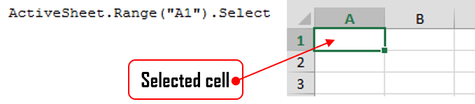
MsgBox Range("B3").Column

---

VBA Select

It is very common to find the .Select methods in saved macro recorder code, next to a Range object.

.Select is used to select one or more elements of Excel (as can be done by using the mouse) allowing further manipulation of them.

Selecting cells with the mouse:

Selecting cells with VBA:

    'Range([cell1],[cell2])
    Range(Cells(1, 1), Cells(9, 5)).Select
    Range("A1", "E9").Select
    Range("A1:E9").Select

Each of the above lines select the range from «A1» to «E9».

---

VBA Select CurrentRegion

If a region is populated by data with no empty cells, an option for an automatic selection is the CurrentRegion property alongside the .Select method.

CurrentRegion.Select will select, starting from a Range, all the area populated with data.

    Range("A1").CurrentRegion.Select

Make sure there are no gaps between values, as CurrentRegion will map the region through adjoining cells (horizontal, vertical and diagonal).

  Range("A1").CurrentRegion.Select

With all the adjacent data

Not all adjacent data

«C4» is not selected because it is not immediately adjacent to any filled cells.

---

VBA ActiveCell

The ActiveCell property brings up the active cell of the worksheet.

In the case of a selection, it is the only cell that stays white.

A worksheet has only one active cell.

    Range("B2:C4").Select
    ActiveCell.Value = "Active"

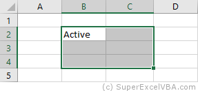
Usually the ActiveCell property is assigned to the first cell (top left) of a Range, although it can be different when the selection is made manually by the user (without macros).

The AtiveCell property can be used with other commands, such as Resize.

---

VBA Selection

After selecting the desired cells, we can use Selection to refer to it and thus make changes:

    Range("A1:D7").Select
    Selection = 7

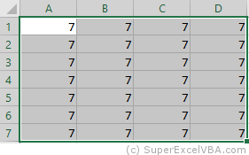
Selection also accepts methods and properties (which vary according to what was selected).

    Selection.ClearContents 'Deletes only the contents of the selection
    Selection.Interior.Color = RGB(255, 255, 0) 'Adds background color to the selection

As in this case a cell range has been selected, the Selection will behave similarly to a Range. Therefore, Selection should also accept the .Interior.Color property.

RGB (Red Green Blue) is a color system used in a number of applications and languages. The input values for each color, in the example case, ranges from 0 to 255.

---

Selection FillDown

If there is a need to replicate a formula to an entire selection, you can use the .FillDown method

    Selection.FillDown

Before the FillDown

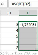
After the FillDown

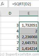
.FillDown is a method applicable to Range. Since the Selection was done in a range of cells (equivalent to a Range), the method will be accepted.

.FillDown replicates the Range/Selection formula of the first line, regardless of which ActiveCell is selected.

.FillDown can be used at intervals greater than one column (E.g. Range(«B1:C2»).FillDown will replicate the formulas of B1 and C1 to B2 and C2 respectively).

---

VBA EntireRow and EntireColumn

You can select one or multiple rows or columns with VBA.

    Range("B2").EntireRow.Select
    Range("C3:D3").EntireColumn.Select

The selection will always refer to the last command executed with Select.

To insert a row use the Insert method.

    Range("A7").EntireRow.Insert
    'In this case, the content of the seventh row will be shifted downward

To delete a row use the Delete method.

    Range("A7").EntireRow.Delete
    'In this case, the content of the eighth row will be moved to the seventh

---

VBA Rows and Columns

Just like with the EntireRow and EntireColumn property, you can use Rows and Columns to select a row or column.

    Columns(5).Select
    Rows(3).Select

To hide rows:

    Range("A1:C3").Rows.Hidden = True

In the above example, rows 1 to 3 of the worksheet were hidden.

---

VBA Row and Column

Row and Column are properties that are often used to obtain the numerical address of the first row or first column of a selection or a specific cell.

    Range("A3:H30").Row 'Referring to the row; returns 3
    Range("B3").Column  'Referring to the column; returns 2

The results of Row and Column are often used in loops or resizing.

---

---

Consolidating Your Learning

Suggested Exercise

---

---

The VBA Range Object

The Excel Range Object is an object in Excel VBA that represents a cell, row, column, a selection of cells or a 3 dimensional range. The Excel Range is also a Worksheet property that returns a subset of its cells.

Worksheet Range

The Range is a Worksheet property which allows you to select any subset of cells, rows, columns etc.

Dim r as Range 'Declared Range variable

Set r = Range("A1") 'Range of A1 cell

Set r = Range("A1:B2") 'Square Range of 4 cells - A1,A2,B1,B2

Set r= Range(Range("A1"), Range ("B1")) 'Range of 2 cells A1 and B1

Range("A1:B2").Select 'Select the Cells A1:B2 in your Excel Worksheet

Range("A1:B2").Activate 'Activate the cells and show them on your screen (will switch to Worksheet and/or scroll to this range.

Select a cell or Range of cells using the Select method. It will be visibly marked in Excel:

Working with Range variables

The Range is a separate object variable and can be declared as other variables. As the VBA Range is an object you need to use the Set statement:

Dim myRange as Range 
'...
Set myRange = Range("A1") 'Need to use Set to define myRange

The Range object defaults to your ActiveWorksheet. So beware as depending on your ActiveWorksheet the Range object will return values local to your worksheet:

Range("A1").Select
'...is the same as...
ActiveSheet.Range("A1").Select

You might want to define the Worksheet reference by Range if you want your reference values from a specifc Worksheet:

Sheets("Sheet1").Range("A1").Select 'Will always select items from Worksheet named Sheet1

The ActiveWorkbook is not same to ThisWorkbook. Same goes for the ActiveSheet. This may reference a Worksheet from within a Workbook external to the Workbook in which the macro is executed as Active references simply the currently top-most worksheet. Read more here

Range properties

The Range object contains a variety of properties with the main one being it’s Value and an the second one being its Formula.

A Range Value is the evaluated property of a cell or a range of cells. For example a cell with the formula =10+20 has an evaluated value of 20.
A Range Formula is the formula provided in the cell or range of cells. For example a cell with a formula of =10+20 will have the same Formula property.

'Let us assume A1 contains the formula "=10+20"

Debug.Print Range("A1").Value 'Returns: 30

Debug.Print Range("A1").Formula 'Returns: =10+20

Other Range properties include:
Work in progress

Worksheet Cells

A Worksheet Cells property is similar to the Range property but allows you to obtain only a SINGLE CELL, based on its row and column index. Numbering starts at 1:

The Cells property is in fact a Range object not a separate data type.
Excel facilitates a Cells function that allows you to obtain a cell from within the ActiveSheet, current top-most worksheet.

Cells(2,2).Select 'Selects B2
'...is the same as...
ActiveSheet.Cells(2,2).Select 'Select B2

Cells are Ranges which means they are not a separate data type:

Dim myRange as Range
Set myRange = Cells(1,1) 'Cell A1

Range Rows and Columns

As we all know an Excel Worksheet is divided into Rows and Columns. The Excel VBA Range object allows you to select single or multiple rows as well as single or multiple columns. There are a couple of ways to obtain Worksheet rows in VBA:

Getting an entire row or column

To get and entire row of a specified Range you need to use the EntireRow property. Although, the function’s parameters suggest taking both a RowIndex and ColumnIndex it is enough just to provide the row number. Row indexing starts at 1.
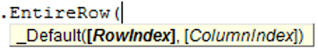To get and entire column of a specified Range you need to use the EntireColumn property. Although, the function’s parameters suggest taking both a RowIndex and ColumnIndex it is enough just to provide the column number. Column indexing starts at 1.

Range("B2").EntireRows(1).Hidden = True 'Gets and hides the entire row 2

Range("B2").EntireColumns(1).Hidden = True 'Gets and hides the entire column 2

The three properties EntireRow/EntireColumn, Rows/Columns and Row/Column are often misunderstood so read through to understand the differences.

Get a row/column of a specified range

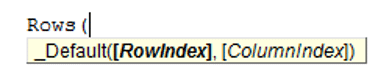If you want to get a certain row within a Range simply use the Rows property of the Worksheet. Although, the function’s parameters suggest taking both a RowIndex and ColumnIndex it is enough just to provide the row number. Row indexing starts at 1.
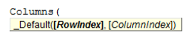Similarly you can use the Columns function to obtain any single column within a Range. Although, the function’s parameters suggest taking both a RowIndex and ColumnIndex actually the first argument you provide will be the column index. Column indexing starts at 1.

Rows(1).Hidden = True 'Hides the first row in the ActiveSheet
'same as
ActiveSheet.Rows(1).Hidden = True

Columns(1).Hidden = True 'Hides the first column in the ActiveSheet
'same as
ActiveSheet.Columns(1).Hidden = True

To get a range of rows/columns you need to use the Range function like so:

Range(Rows(1), Rows(3)).Hidden = True 'Hides rows 1:3
'same as
Range("1:3").Hidden = True
'same as 
ActiveSheet.Range("1:3").Hidden = True

Range(Columns(1), Columns(3)).Hidden = True 'Hides columns A:C
'same as
Range("A:C").Hidden = True
'same as 
ActiveSheet.Range("A:C").Hidden = True

Get row/column of specified range

The above approach assumed you want to obtain only rows/columns from the ActiveSheet – the visible and top-most Worksheet. Usually however, you will want to obtain rows or columns of an existing Range. Similarly as with the Worksheet Range property, any Range facilitates the Rows and Columns property.

Dim myRange as Range
Set myRange = Range("A1:C3")

myRange.Rows.Hidden = True 'Hides rows 1:3
myRange.Columns.Hidden = True 'Hides columns A:C

Set myRange = Range("C10:F20")
myRange.Rows(2).Hidden = True 'Hides rows 11
myRange.Columns(3).Hidden = True 'Hides columns E

Getting a Ranges first row/column number

Aside from the Rows and Columns properties Ranges also facilitate a Row and Column property which provide you with the number of the Ranges first row and column.

Set myRange = Range("C10:F20")

'Get first row number
Debug.Print myRange.Row 'Result: 10
'Get first column number
Debug.Print myRange.Column 'Result: 3

Converting Column number to Excel Column

This is an often question that turns up – how to convert a column number to a string e.g. 100 to “CV”.

Function GetExcelColumn(columnNumber As Long)
    Dim div As Long, colName As String, modulo As Long
    div = columnNumber: colName = vbNullString

    Do While div > 0
        modulo = (div - 1) Mod 26
        colName = Chr(65 + modulo) & colName
        div = ((div - modulo) / 26)
    Loop

    GetExcelColumn = colName
End Function

Range Cut/Copy/Paste

Cutting and pasting rows is generally a bad practice which I heavily discourage as this is a practice that is moments can be heavily cpu-intensive and often is unaccounted for.

Copy function

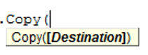The Copy function works on a single cell, subset of cell or subset of rows/columns.

'Copy values and formatting from cell A1 to cell D1
Range("A1").Copy Range("D1")

'Copy 3x3 A1:C3 matrix to D1:F3 matrix - dimension must be same
Range("A1:C3").Copy Range("D1:F3")

'Copy rows 1:3 to rows 4:6
Range("A1:A3").EntireRow.Copy Range("A4")

'Copy columns A:C to columns D:F
Range("A1:C1").EntireColumn.Copy Range("D1")

The Copy function can also be executed without an argument. It then copies the Range to the Windows Clipboard for later Pasting.

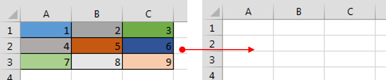
Cut function

The Cut function, similarly as the Copy function, cuts single cells, ranges of cells or rows/columns.

'Cut A1 cell and paste it to D1
Range("A1").Cut Range("D1")

'Cut 3x3 A1:C3 matrix and paste it in D1:F3 matrix - dimension must be same
Range("A1:C3").Cut Range("D1:F3")

'Cut rows 1:3 and paste to rows 4:6
Range("A1:A3").EntireRow.Cut Range("A4")

'Cut columns A:C and paste to columns D:F
Range("A1:C1").EntireColumn.Cut Range("D1")

The Cut function can be executed without arguments. It will then cut the contents of the Range and copy it to the Windows Clipboard for pasting.

Cutting cells/rows/columns does not shift any remaining cells/rows/columns but simply leaves the cut out cells empty

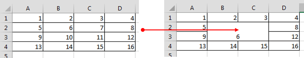
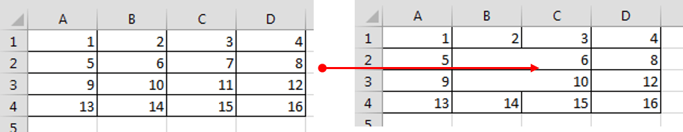
PasteSpecial function

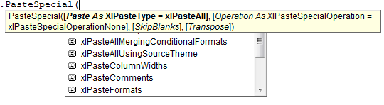The Range PasteSpecial function works only when preceded with either the Copy or Cut Range functions. It pastes the Range (or other data) within the Clipboard to the Range on which it was executed.

Syntax

The PasteSpecial function has the following syntax:

PasteSpecial( Paste, Operation, SkipBlanks, Transpose)

The PasteSpecial function can only be used in tandem with the Copy function (not Cut)

Parameters

Paste
The part of the Range which is to be pasted. This parameter can have the following values:

Parameter	Constant	Description
xlPasteSpecialOperationAdd	2	Copied data will be added with the value in the destination cell.
xlPasteSpecialOperationDivide	5	Copied data will be divided with the value in the destination cell.
xlPasteSpecialOperationMultiply	4	Copied data will be multiplied with the value in the destination cell.
xlPasteSpecialOperationNone	-4142	No calculation will be done in the paste operation.
xlPasteSpecialOperationSubtract	3	Copied data will be subtracted with the value in the destination cell.

Operation
The paste operation e.g. paste all, only formatting, only values, etc. This can have one of the following values:

Name	Constant	Description
xlPasteAll	-4104	Everything will be pasted.
xlPasteAllExceptBorders	7	Everything except borders will be pasted.
xlPasteAllMergingConditionalFormats	14	Everything will be pasted and conditional formats will be merged.
xlPasteAllUsingSourceTheme	13	Everything will be pasted using the source theme.
xlPasteColumnWidths	8	Copied column width is pasted.
xlPasteComments	-4144	Comments are pasted.
xlPasteFormats	-4122	Copied source format is pasted.
xlPasteFormulas	-4123	Formulas are pasted.
xlPasteFormulasAndNumberFormats	11	Formulas and Number formats are pasted.
xlPasteValidation	6	Validations are pasted.
xlPasteValues	-4163	Values are pasted.
xlPasteValuesAndNumberFormats	12	Values and Number formats are pasted.

SkipBlanks
If True then blanks will not be pasted.

Transpose
Transpose the Range before paste (swap rows with columns).

PasteSpecial Examples

'Cut A1 cell and paste its values to D1
Range("A1").Copy
Range("D1").PasteSpecial
 
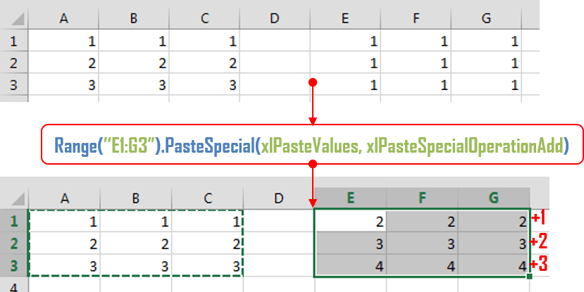
'Copy 3x3 A1:C3 matrix and add all the values to E1:G3 matrix (dimension must be same)
Range("A1:C3").Copy 
Range("E1:G3").PasteSpecial xlPasteValues, xlPasteSpecialOperationAdd

Below an example where the Excel Range A1:C3 values are copied an added to the E1:G3 Range. You can also multiply, divide and run other similar operations.

Paste

The Paste function allows you to paste data in the Clipboard to the actively selected Range. Cutting and Pasting can only be accomplished with the Paste function.

'Cut A1 cell and paste its values to D1
Range("A1").Cut
Range("D1").Select
ActiveSheet.Paste
 
'Cut 3x3 A1:C3 matrix and paste it in D1:F3 matrix - dimension must be same
Range("A1:C3").Cut 
Range("D1:F3").Select
ActiveSheet.Paste
 
'Cut rows 1:3 and paste to rows 4:6
Range("A1:A3").EntireRow.Cut 
Range("A4").Select
ActiveSheet.Paste
 
'Cut columns A:C and paste to columns D:F
Range("A1:C1").EntireColumn.Cut 
Range("D1").Select
ActiveSheet.Paste

Range Clear/Delete

The Clear function

The Clear function clears the entire content and formatting from an Excel Range. It does not, however, shift (delete) the cleared cells.

Range("A1:C3").Clear

The Delete function

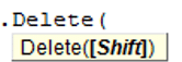The Delete function deletes a Range of cells, removing them entirely from the Worksheet, and shifts the remaining Cells in a selected shift direction.
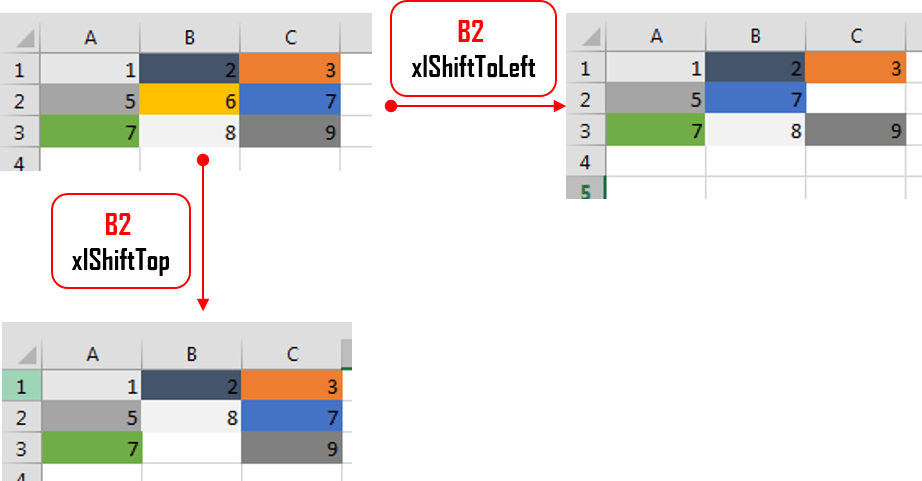
Although the manual Delete cell function provides 4 ways of shifting cells. The VBA Delete Shift values can only be either be xlShiftToLeft or xlShiftUp.

'If Shift omitted, Excel decides - shift up in this case
Range("B2").Delete 

'Delete and Shift remaining cells left
Range("B2").Delete xlShiftToLeft  

'Delete and Shift remaining cells up
Range("B2").Delete xlShiftTop

'Delete entire row 2 and shift up
Range("B2").EntireRow.Delete

'Delete entire column B and shift left
Range("B2").EntireRow.Delete

Traversing Ranges

Traversing cells is really useful when you want to run an operation on each cell within an Excel Range. Fortunately this is easily achieved in VBA using the For Each or For loops.

Dim cellRange As Range
    
For Each cellRange In Range("A1:C3")
  Debug.Print cellRange.Value
Next cellRange

Although this may not be obvious, beware of iterating/traversing the Excel Range using a simple For loop. For loops are not efficient on Ranges. Use a For Each loop as shown above. This is because Ranges resemble more Collections than Arrays. Read more on For vs For Each loops here

Traversing the UsedRange

Every Worksheet has a UsedRange. This represents that smallest rectangle Range that contains all cells that have or had at some point values. In other words if the further out in the bottom, right-corner of the Worksheet there is a certain cell (e.g. E8) then the UsedRange will be as large as to include that cell starting at cell A1 (e.g. A1:E8). In Excel you can check the current UsedRange hitting CTRL+END. In VBA you get the UsedRange like this:

ActiveSheet.UsedRange
'same as
UsedRange

You can traverse through the UsedRange like this:

Dim cellRange As Range
    
For Each cellRange In UsedRange
  Debug.Print "Row: " & cellRange.Row & ", Column: " & cellRange.Column
Next cellRange

The UsedRange is a useful construct responsible often for bloated Excel Workbooks. Often delete unused Rows and Columns that are considered to be within the UsedRange can result in significantly reducing your file size. Read also more on the XSLB file format here

Range Addresses

The Excel Range Address property provides a string value representing the Address of the Range.

Syntax

Below the syntax of the Excel Range Address property:

Address( [RowAbsolute], [ColumnAbsolute], [ReferenceStyle], [External], [RelativeTo] )

Parameters

RowAbsolute
Optional. If True returns the row part of the reference address as an absolute reference. By default this is True.

$D$10:$G$100 'RowAbsolute is set to True
$D10:$G100 'RowAbsolute is set to False

ColumnAbsolute
Optional. If True returns the column part of the reference as an absolute reference. By default this is True.

$D$10:$G$100 'ColumnAbsolute is set to True
D$10:G$100 'ColumnAbsolute is set to False

ReferenceStyle
Optional. The reference style. The default value is xlA1. Possible values:

Constant	Value	Description
xlA1	1	Default. Use xlA1 to return an A1-style reference
xlR1C1	-4150	Use xlR1C1 to return an R1C1-style reference

External
Optional. If True then property will return an external reference address, otherwise a local reference address will be returned. By default this is False.

$A$1 'Local
[Book1.xlsb]Sheet1!$A$1 'External

RelativeTo
Provided RowAbsolute and ColumnAbsolute are set to False, and the ReferenceStyle is set to xlR1C1, then you must include a starting point for the relative reference. This must be a Range variable to be set as the reference point.

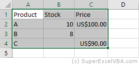
Merged Ranges

Merged cells are Ranges that consist of 2 or more adjacent cells. To Merge a collection of adjacent cells run Merge function on that Range.

The Merge has only a single parameter – Across, a boolean which if True will merge cells in each row of the specified range as separate merged cells. Otherwise the whole Range will be merged. The default value is False.

Merge examples

To merge the entire Range:

'This will turn of any alerts warning that values may be lost
Application.DisplayAlerts = False

Range("B2:C3").Merge

This will result in the following:

To merge just the rows set Across to True.

'This will turn of any alerts warning that values may be lost
Application.DisplayAlerts = False

Range("B2:C3").Merge True

This will result in the following:

Remember that merged Ranges can only have a single value and formula. Hence, if you merge a group of cells with more than a single value/formula only the first value/formula will be set as the value/formula for your new merged Range

Checking if Range is merged

To check if a certain Range is merged simply use the Excel Range MergeCells property:

Range("B2:C3").Merge

Debug.Print Range("B2").MergeCells 'Result: True

The MergeArea

The MergeArea is a property of an Excel Range that represent the whole merge Range associated with the current Range. Say that $B$2:$C$3 is a merged Range – each cell within that Range (e.g. B2, C3..) will have the exact same MergedArea. See example below:

Range("B2:C3").Merge
Debug.Print Range("B2").MergeArea.Address 'Result: $B$2:$C$3

Named Ranges

Named Ranges are Ranges associated with a certain Name (string). In Excel you can find all your Named Ranges by going to Formulas->Name Manager. They are very useful when working on certain values that are used frequently through out your Workbook. Imagine that you are writing a Financial Analysis and want to use a common Discount Rate across all formulas. Just the address of the cell e.g. “A2”, won’t be self-explanatory. Why not use e.g. “DiscountRate” instead? Well you can do just that.

Creating a Named Range

Named Ranges can be created either within the scope of a Workbook or Worksheet:

Dim r as Range
'Within Workbook
Set r = ActiveWorkbook.Names.Add("NewName", Range("A1"))
'Within Worksheet
Set r = ActiveSheet.Names.Add("NewName", Range("A1"))

This gives you flexibility to use similar names across multiple Worksheets or use a single global name across the entire Workbook.

Listing all Named Ranges

You can list all Named Ranges using the Name Excel data type. Names are objects that represent a single NamedRange. See an example below of listing our two newly created NamedRanges:

Call ActiveWorkbook.Names.Add("NewName", Range("A1"))
Call ActiveSheet.Names.Add("NewName", Range("A1"))

Dim n As Name
For Each n In ActiveWorkbook.Names
  Debug.Print "Name: " & n.Name & ", Address: " & _
       n.RefersToRange.Address & ", Value: "; n.RefersToRange.Value
Next n

'Result:
'Name: Sheet1!NewName, Address: $A$1, Value:  1 
'Name: NewName, Address: $A$1, Value:  1 

SpecialCells

SpecialCells are a very useful Excel Range property, that allows you to select a subset of cells/Ranges within a certain Range.

Syntax

The SpecialCells property has the following syntax:

SpecialCells( Type, [Value] )

Parameters

Type
The type of cells to be returned. Possible values:

Constant	Value	Description
xlCellTypeAllFormatConditions	-4172	Cells of any format
xlCellTypeAllValidation	-4174	Cells having validation criteria
xlCellTypeBlanks	4	Empty cells
xlCellTypeComments	-4144	Cells containing notes
xlCellTypeConstants	2	Cells containing constants
xlCellTypeFormulas	-4123	Cells containing formulas
xlCellTypeLastCell	11	The last cell in the used range
xlCellTypeSameFormatConditions	-4173	Cells having the same format
xlCellTypeSameValidation	-4175	Cells having the same validation criteria
xlCellTypeVisible	12	All visible cells

Value
If Type is equal to xlCellTypeConstants or xlCellTypeFormulas this determines the types of cells to return e.g. with errors.

Constant	Value
xlErrors	16
xlLogical	4
xlNumbers	1
xlTextValues	2

SpecialCells examples

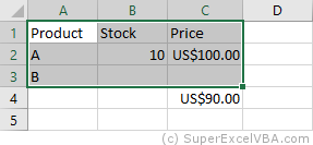
Get Excel Range with Constants

This will return only cells with constant cells within the Range C1:C3:

For Each r In Range("A1:C3").SpecialCells(xlCellTypeConstants)
  Debug.Print r.Value
Next r

Search for Excel Range with Errors

For Each r In ActiveSheet.UsedRange.SpecialCells(xlCellTypeFormulas, xlErrors)
  Debug.Print r.Address
Next r

Продолжаем наш разговор про объект Excel Range, начатый в первой части. Разберём ещё несколько типовых задач и одну развлекательную. Кстати, в процессе написания второй части я дополнил и расширил первую, поэтому рекомендую её посмотреть ещё раз.

Примеры кода

Скачать

Типовые задачи

1. Перебор ячеек диапазона (вариант 4)

   Для коллекции добавил четвёртый вариант перебора ячеек. Как видите, можно выбирать, как перебирается диапазон — по столбцам или по строкам. Обратите внимание на использование свойства коллекции Cells. Не путайте: свойство Cells рабочего листа содержит все ячейки листа, а свойство Cells диапазона (Range) содержит ячейки только этого диапазона. В данном случае мы получаем все ячейки столбца или строки.

   Sub Handle_Cells_4_by_Columns(parRange As Range)
     For Each columnTemp In parRange.Columns
       For Each cellTemp In columnTemp.Cells
         Sum = Sum + cellTemp
       Next
     Next
     MsgBox "Сумма ячеек " & Sum
   End Sub
   
   Sub Handle_Cells_4_by_Rows(parRange As Range)
     For Each rowTemp In parRange.Rows
       For Each cellTemp In rowTemp.Cells
         Sum = Sum + cellTemp
       Next
     Next
     MsgBox "Сумма ячеек " & Sum
   End Sub
    

   Должен вас предупредить, что код, который вы видите в этом цикле статей — это код, написанный для целей демонстрации работы с объектной моделью Excel. Тут нет объявлений переменных, обработки ошибок и проверки условий, так как я специально минимизирую программы, пытаясь акцентировать ваше внимание целиком на обсуждаемом предмете — объекте Range.

2. Работа с текущей областью

   Excel умеет автоматически определять текущую область вокруг активной ячейки. Соответствующая команда на листе вызывается через Ctrl+A. Через ActiveCell мы посредством свойства Worksheet легко выходим на лист текущей ячейки, а уже через него можем эксплуатировать свойство UsedRange, которое и является ссылкой на Range текущей области. Чтобы понять, какой диапазон мы получили, мы меняем цвет ячеек. Функция GetRandomColor не является стандартной, она определена в модуле файла примера.

   ActiveCell.Worksheet.UsedRange.Interior.Color = GetRandomColor
    

3. Определение границ текущей области

   Демонстрируем определение левого верхнего и правого нижнего углов диапазона текущей области. С левым верхним углом всё просто, так как координаты этой ячейки всегда доступны через свойства Row и Column объекта Range (не путать с коллекциями Rows и Columns!). А вот для определения второго угла приходится использовать конструкцию вида .Rows(.Rows.Count).Row, где .Rows.Count — количество строк в диапазоне UsedRange, .Rows(.Rows.Count) — это мы получили последнюю строку, и уже для этого диапазона забираем из свойства Row координату строки. Со столбцом — по аналогии. Также обратите внимание на использование оператора With. Как видите, оператор With, помимо сокращения кода, также позволяет отказаться от объявления отдельной объектной переменной через оператор Set, что очень удобно.

   With ActiveCell.Worksheet.UsedRange
     strTemp = "Верхняя строка " & vbTab & .Row & vbCr & _
               "Нижняя строка " & vbTab & .Rows(.Rows.Count).Row & vbCr & _
               "Левый столбец " & vbTab & .Column & vbCr & _
               "Правый столбец " & vbTab & .Columns(.Columns.Count).Column
   End With
   MsgBox strTemp, vbInformation
    

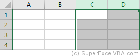
4. Выделение столбцов / строк текущей области

   Тут нет ничего нового, мы всё это обсудили в предыдущем примере. Мы получаем ссылки на столбцы / строки, меняя их цвет для контроля результата работы кода.

   With ActiveCell.Worksheet.UsedRange
     .Rows(1).Interior.Color = GetRandomColor
     .Rows(.Rows.Count).Interior.Color = GetRandomColor
   End With
    

   With ActiveCell.Worksheet.UsedRange
     .Columns(1).Interior.Color = GetRandomColor
     .Columns(.Columns.Count).Interior.Color = GetRandomColor
   End With
    

5. Сброс форматирования диапазона

   Для возвращения диапазона к каноническому стерильному состоянию очень просто и удобно использовать свойство Style, и присвоить ему имя стиля «Normal». Интересно, что все остальные стандартные стили в локализованном офисе имеют русские имена, а у этого стиля оставили англоязычное имя, что неплохо.

   ActiveCell.Worksheet.UsedRange.Style = "Normal"
    

6. Поиск последней строки столбца (вариант 1)

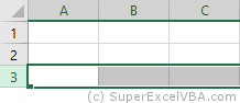
   Range имеет 2 свойства EntireColumn и EntireRow, возвращающие столбцы / строки, на которых расположился ваш диапазон, но возвращают их ЦЕЛИКОМ. То есть, если вы настроили диапазон на D5, то Range(«D5»).EntireColumn вернёт вам ссылку на D:D, а EntireRow — на 5:5.

   Идём далее — свойство End возвращает вам ближайшую ячейку в определенном направлении, стоящую на границе непрерывного диапазона с данными. Как это работает вы можете увидеть, нажимая на листе комбинации клавиш Ctrl+стрелки. Кстати, это одна из самых полезных горячих клавиш в Excel. Направление задаётся стандартными константами xlUp, xlDown, xlToRight, xlToLeft.

   Классическая задача у Excel программиста — определить, где кончается таблица или, в данном случае, конкретный столбец. Идея состоит в том, чтобы встать на последнюю ячейку столбца (строка 1048576) и, стоя в этой ячейке, перейти по Ctrl+стрелка вверх (что на языке VBA — End(xlUp)).

   With ActiveCell.EntireColumn
     .Cells(.Rows.Count, 1).End(xlUp).Select
   End With
    

7. Поиск последней строки столбца (вариант 2)

   Ещё один вариант.

   With ActiveCell.Worksheet
     .Cells(.Rows.Count, ActiveCell.Column).End(xlUp).Select
   End With
    

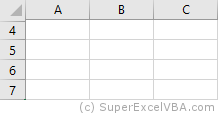
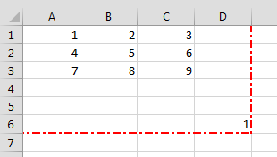
8. Поиск «последней» ячейки листа

   Тут показывается, как найти на листе ячейку, ниже и правее которой находятся только пустые ячейки. Соответственно данные надо искать в диапазоне от A1 до этой ячейки. На эту ячейку можно перейти через Ctrl+End. Как этим воспользоваться в VBA показано ниже:

   ActiveCell.Worksheet.Cells.SpecialCells(xlCellTypeLastCell).Select
    

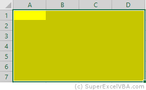
9. Разбор клипо-генератора

   Ну, и в качестве развлечения и разрядки взгляните на код клипо-генератора, который генерирует цветные квадраты в заданных границах экрана. На некоторых это оказывает умиротворяющий эффект

   

   По нашей теме в коде обращает на себя внимание использование свойства ReSize объекта Range. Как не трудно догадаться, свойство расширяет (усекает) текущий диапазон до указанных границ, при этом левый верхний угол диапазона сохраняет свои координаты. А также посмотрите на 2 последние строчки кода, реализующие очистку экрана. Там весьма показательно использован каскад свойств End и Offset.

   Sub Indicator(start As Range)
   
     ' выясняем границы "экрана" (чёрная рамка с ячейками =1)
     LimitUp = start.End(xlUp).Row
     LimitDown = start.End(xlDown).Row
     LimitRight = start.End(xlToRight).Column
     LimitLeft = start.End(xlToLeft).Column
     
     ' бесконечный цикл, пока пользователь не нажал кнопку "Стоп"
     Do While Not PleaseStop
     
       ' размер клипа может меняться счётчиком, поэтому обновляем из ИД
       MinSize = Range("rngSize")
     
       iColor = GetRandomColor ' получаем случайный цвет для "клипа"
     
       ' верхний угол "клипа"
       iTop = LimitUp + Int(Rnd * (LimitDown - LimitUp - MinSize)) + 1
       
       ' левый угол "клипа"
       iLeft = LimitLeft + Int(Rnd * (LimitRight - LimitLeft - MinSize)) + 1
       
       ' выводим "клип" на экран, закрашивая фон диапазона
       ' размер диапазона - квадрат со стороной MinSize
       Cells(iTop, iLeft).Resize(MinSize, MinSize).Interior.Color = iColor
       
       ' Задержка между клипами зависит от MinSize, 5 - в миллисекундах
       Sleep 5 * MinSize
       
       DoEvents ' даём операционной системе и приложениям нормально функционировать
       
     Loop
     
     ' после завершения цикла переходим в верхний левый угол экрана
     start.End(xlUp).End(xlToLeft).Offset(1, 1).Select
     ' выделяем "экран" и очищаем его через изменния стиля ячеек
     Range(Selection, Selection.End(xlToRight).End(xlDown).Offset(-1, -1)).Style = "Normal"
     
   End Sub
    

Читайте также:

• Работа с объектом Range

• Массивы в VBA

• Структуры данных и их эффективность

• Автоматическое скрытие/показ столбцов и строк