
Содержание
- Свойство Worksheet.Cells (Excel)
- Синтаксис
- Замечания
- Пример
- Поддержка и обратная связь
- Worksheet_Change — Targeting multiple cells simultaneously
- 2 Answers 2
- Formatting a Range of Cells In Excel VBA
- Formatting Cells Number
- General
- Number
- Currency
- Accounting
- Percentage
- Fraction
- Scientific
- Special
- Custom
- Formatting Cells Alignment
- Text Alignment
- Horizontal
- Vertical
- Text Control
- Wrap Text
- Shrink To Fit
- Merge Cells
- Right-to-left
- Text direction
- Orientation
- Font Name
- Font Style
- Font Size
- Underline
- Font Color
- Font Effects
- Strikethrough
- Subscript
- Superscript
- Border
- Border Index
- Line Style
- Line Thickness
- Line Color
- Pattern Style
- Protection
- Locking Cells
- Hiding Formulas
- Working with Cells and Ranges in Excel VBA (Select, Copy, Move, Edit)
- Selecting a Cell / Range in Excel using VBA
- Selecting a Single Cell Using VBA
- Selecting a Fix Sized Range
- Selecting a Variably Sized Range
- Select Using CurrentRange Property
- Select Using UsedRange Property
- Select Using the End Property
- Difference between Using CurrentRegion and End
- Copy Cells / Ranges Using VBA
- Copying Single Cell
- Copying a Fix Sized Range
- Copying a Variable Sized Range
- Assigning Ranges to Object Variables
- Enter Data in the Next Empty Cell (Using Input Box)
- Looping Through Cells / Ranges
- Where to Put the VBA Code
Свойство Worksheet.Cells (Excel)
Возвращает объект Range , представляющий все ячейки на листе (а не только используемые в данный момент ячейки).
Синтаксис
выражение.Cells
Выражение Переменная, представляющая объект Worksheet .
Замечания
Так как элемент по умолчанию объекта Range направляет вызовы с параметрами в свойство Item, можно указать индекс строки и столбца сразу после ключевого слова Cells, вместо явного вызова свойства Item.
При использовании этого свойства без квалификатора объекта возвращается объект Range, который представляет все ячейки на активном листе.
Пример
В этом примере размер шрифта ячейки C5 на листе 1 активной книги устанавливается в 14 пунктов.
В этом примере формула очищается в ячейке 1 на листе 1 активной книги.
В этом примере шрифт и размер шрифта для каждой ячейки на листе Sheet1 устанавливается значение Arial из 8 точек.
В этом примере выполняется переключение сортировки между порядком по возрастанию и убыванию при двойном щелчке любой ячейки в диапазоне данных. Данные сортируются по столбцу ячейки, дважды щелкнув которую.
В этом примере выполняется просмотр столбца C активного листа, и для каждой ячейки с комментарием текст примечания помещается в столбец D и удаляется комментарий из столбца C.
Поддержка и обратная связь
Есть вопросы или отзывы, касающиеся Office VBA или этой статьи? Руководство по другим способам получения поддержки и отправки отзывов см. в статье Поддержка Office VBA и обратная связь.
Источник
Worksheet_Change — Targeting multiple cells simultaneously
VBA beginner here.
I have project where I have specified input cells for the user. When one of these input cells is changed, it needs to run a few lines of code that are specific to only that one cell. If the user clears the contents of the cell, I want the code to replace the blank cell with the value «0».
The code below simulates what I am trying to achieve. It is written in the same form as my project but is more succinct.
Everything above works fine when the changes are performed on single cells. If the user selects all the cells and presses the delete key, it only runs the code for the first cell. I want it to run for all the selected (deleted) cells.
Any advice on how to simultaneously run the Worksheet_Change across multiple cells?
2 Answers 2
When you have a change event that works just fine on a single cell, you can make a few adjustments to ensure that it also works when you change a range of cells in one go, like when you paste three cells into A1 to A3
You may want to apply an approach similar to this:
If Not Intersect(Target, Range(«A1:A3»)) Is Nothing Then — only act on changes to cells A1 to A3
For Each cel In Target — do the same thing for all cells that have been changed
Range(«B» & myRow).Value = «Changed » & Target.Row — enter some value into column B of the current row
In the next step of the macro we will possibly enter some data into the cells we are monitoring for a change, i.e. A1 to A3. A change in these cells will trigger this macro. This macro will write into the cells. A change in the cells will trigger this macro .
You see where this is going. In order to avoid an endless loop, we turn off any event triggered macros, e.g. macros that fire when a cell is changed. So we turn off event monitoring with this statement.
Application.EnableEvents = False — Now any events like «a cell has been changed» will be ignored.
We can now write a value into column A and that will not trigger the macro again. Great. We do whatever we need to do to cells A1 to A3 and then we turn event monitoring back on.
Then we go to the next cell (if any) in the range that triggered this macro.
Let me know if that helps or if you need a bit more detail. These things take a little learning curve.
Источник
Formatting a Range of Cells In Excel VBA
Formatting Cells Number
General
Number
Currency
Accounting
Percentage
Fraction
Scientific
Special
Custom
Formatting Cells Alignment
Text Alignment
Horizontal
The value of this property can be set to one of the constants: xlGeneral, xlCenter, xlDistributed, xlJustify, xlLeft, xlRight.
The following code sets the horizontal alignment of cell A1 to center.
Vertical
The value of this property can be set to one of the constants: xlBottom, xlCenter, xlDistributed, xlJustify, xlTop.
The following code sets the vertical alignment of cell A1 to bottom.
Text Control
Wrap Text
This example formats cell A1 so that the text wraps within the cell.
Shrink To Fit
This example causes text in row one to automatically shrink to fit in the available column width.
Merge Cells
This example merge range A1:A4 to a large one.
Right-to-left
Text direction
The value of this property can be set to one of the constants: xlRTL (right-to-left), xlLTR (left-to-right), or xlContext (context).
The following code example sets the reading order of cell A1 to xlRTL (right-to-left).
Orientation
The value of this property can be set to an integer value from –90 to 90 degrees or to one of the following constants: xlDownward, xlHorizontal, xlUpward, xlVertical.
The following code example sets the orientation of cell A1 to xlHorizontal.
Font Name
The value of this property can be set to one of the fonts: Calibri, Times new Roman, Arial.
The following code sets the font name of range A1:A5 to Calibri.
Font Style
The value of this property can be set to one of the constants: Regular, Bold, Italic, Bold Italic.
The following code sets the font style of range A1:A5 to Italic.
Font Size
The value of this property can be set to an integer value from 1 to 409.
The following code sets the font size of cell A1 to 14.
Underline
The value of this property can be set to one of the constants: xlUnderlineStyleNone, xlUnderlineStyleSingle, xlUnderlineStyleDouble, xlUnderlineStyleSingleAccounting, xlUnderlineStyleDoubleAccounting.
The following code sets the font of cell A1 to xlUnderlineStyleDouble (double underline).
Font Color
The value of this property can be set to one of the standard colors: vbBlack, vbRed, vbGreen, vbYellow, vbBlue, vbMagenta, vbCyan, vbWhite or an integer value from 0 to 16,581,375.
To assist you with specifying the color of anything, the VBA is equipped with a function named RGB. Its syntax is:
This function takes three arguments and each must hold a value between 0 and 255. The first argument represents the ratio of red of the color. The second argument represents the green ratio of the color. The last argument represents the blue of the color. After the function has been called, it produces a number whose maximum value can be 255 * 255 * 255 = 16,581,375, which represents a color.
The following code sets the font color of cell A1 to vbBlack (Black).
The following code sets the font color of cell A1 to 0 (Black).
The following code sets the font color of cell A1 to RGB(0, 0, 0) (Black).
Font Effects
Strikethrough
True if the font is struck through with a horizontal line.
The following code sets the font of cell A1 to strikethrough.
Subscript
True if the font is formatted as subscript. False by default.
The following code sets the font of cell A1 to Subscript.
Superscript
True if the font is formatted as superscript; False by default.
The following code sets the font of cell A1 to Superscript.
Border
Border Index
Using VBA you can choose to create borders for the different edges of a range of cells:
- xlDiagonalDown (Border running from the upper left-hand corner to the lower right of each cell in the range).
- xlDiagonalUp (Border running from the lower left-hand corner to the upper right of each cell in the range).
- xlEdgeBottom (Border at the bottom of the range).
- xlEdgeLeft (Border at the left-hand edge of the range).
- xlEdgeRight (Border at the right-hand edge of the range).
- xlEdgeTop (Border at the top of the range).
- xlInsideHorizontal (Horizontal borders for all cells in the range except borders on the outside of the range).
- xlInsideVertical (Vertical borders for all the cells in the range except borders on the outside of the range).
Line Style
The value of this property can be set to one of the constants: xlContinuous (Continuous line), xlDash (Dashed line), xlDashDot (Alternating dashes and dots), xlDashDotDot (Dash followed by two dots), xlDot (Dotted line), xlDouble (Double line), xlLineStyleNone (No line), xlSlantDashDot (Slanted dashes).
The following code example sets the border on the bottom edge of cell A1 with continuous line.
The following code example removes the border on the bottom edge of cell A1.
Line Thickness
The value of this property can be set to one of the constants: xlHairline (Hairline, thinnest border), xlMedium (Medium), xlThick (Thick, widest border), xlThin (Thin).
The following code example sets the thickness of the border created to xlThin (Thin).
Line Color
The value of this property can be set to one of the standard colors: vbBlack, vbRed, vbGreen, vbYellow, vbBlue, vbMagenta, vbCyan, vbWhite or an integer value from 0 to 16,581,375.
The following code example sets the color of the border on the bottom edge to green.
You can also use the RGB function to create a color value.
The following example sets the color of the bottom border of cell A1 with RGB fuction.
Pattern Style
The value of this property can be set to one of the constants:
- xlPatternAutomatic (Excel controls the pattern.)
- xlPatternChecker (Checkerboard.)
- xlPatternCrissCross (Criss-cross lines.)
- xlPatternDown (Dark diagonal lines running from the upper left to the lower right.)
- xlPatternGray16 (16% gray.)
- xlPatternGray25 (25% gray.)
- xlPatternGray50 (50% gray.)
- xlPatternGray75 (75% gray.)
- xlPatternGray8 (8% gray.)
- xlPatternGrid (Grid.)
- xlPatternHorizontal (Dark horizontal lines.)
- xlPatternLightDown (Light diagonal lines running from the upper left to the lower right.)
- xlPatternLightHorizontal (Light horizontal lines.)
- xlPatternLightUp (Light diagonal lines running from the lower left to the upper right.)
- xlPatternLightVertical (Light vertical bars.)
- xlPatternNone (No pattern.)
- xlPatternSemiGray75 (75% dark moiré.)
- xlPatternSolid (Solid color.)
- xlPatternUp (Dark diagonal lines running from the lower left to the upper right.)
Protection
Locking Cells
This property returns True if the object is locked, False if the object can be modified when the sheet is protected, or Null if the specified range contains both locked and unlocked cells.
The following code example unlocks cells A1:B22 on Sheet1 so that they can be modified when the sheet is protected.
Hiding Formulas
This property returns True if the formula will be hidden when the worksheet is protected, Null if the specified range contains some cells with FormulaHidden equal to True and some cells with FormulaHidden equal to False.
Don’t confuse this property with the Hidden property. The formula will not be hidden if the workbook is protected and the worksheet is not, but only if the worksheet is protected.
The following code example hides the formulas in cells A1 and C1 on Sheet1 when the worksheet is protected.
Источник
Working with Cells and Ranges in Excel VBA (Select, Copy, Move, Edit)
When working with Excel, most of your time is spent in the worksheet area – dealing with cells and ranges.
And if you want to automate your work in Excel using VBA, you need to know how to work with cells and ranges using VBA.
There are a lot of different things you can do with ranges in VBA (such as select, copy, move, edit, etc.).
So to cover this topic, I will break this tutorial into sections and show you how to work with cells and ranges in Excel VBA using examples.
Let’s get started.
If you’re interested in learning VBA the easy way, check out my Online Excel VBA Training.
This Tutorial Covers:
Selecting a Cell / Range in Excel using VBA
To work with cells and ranges in Excel using VBA, you don’t need to select it.
In most of the cases, you are better off not selecting cells or ranges (as we will see).
Despite that, it’s important you go through this section and understand how it works. This will be crucial in your VBA learning and a lot of concepts covered here will be used throughout this tutorial.
So let’s start with a very simple example.
Selecting a Single Cell Using VBA
If you want to select a single cell in the active sheet (say A1), then you can use the below code:
The above code has the mandatory ‘Sub’ and ‘End Sub’ part, and a line of code that selects cell A1.
Range(“A1”) tells VBA the address of the cell that we want to refer to.
Select is a method of the Range object and selects the cells/range specified in the Range object. The cell references need to be enclosed in double quotes.
This code would show an error in case a chart sheet is an active sheet. A chart sheet contains charts and is not widely used. Since it doesn’t have cells/ranges in it, the above code can’t select it and would end up showing an error.
Note that since you want to select the cell in the active sheet, you just need to specify the cell address.
But if you want to select the cell in another sheet (let’s say Sheet2), you need to first activate Sheet2 and then select the cell in it.
Similarly, you can also activate a workbook, then activate a specific worksheet in it, and then select a cell.
Note that when you refer to workbooks, you need to use the full name along with the file extension (.xlsx in the above code). In case the workbook has never been saved, you don’t need to use the file extension.
Now, these examples are not very useful, but you will see later in this tutorial how we can use the same concepts to copy and paste cells in Excel (using VBA).
Just as we select a cell, we can also select a range.
In case of a range, it could be a fixed size range or a variable size range.
In a fixed size range, you would know how big the range is and you can use the exact size in your VBA code. But with a variable-sized range, you have no idea how big the range is and you need to use a little bit of VBA magic.
Let’s see how to do this.
Selecting a Fix Sized Range
Here is the code that will select the range A1:D20.
Another way of doing this is using the below code:
The above code takes the top-left cell address (A1) and the bottom-right cell address (D20) and selects the entire range. This technique becomes useful when you’re working with variably sized ranges (as we will see when the End property is covered later in this tutorial).
If you want the selection to happen in a different workbook or a different worksheet, then you need to tell VBA the exact names of these objects.
For example, the below code would select the range A1:D20 in Sheet2 worksheet in the Book2 workbook.
Now, what if you don’t know how many rows are there. What if you want to select all the cells that have a value in it.
In these cases, you need to use the methods shown in the next section (on selecting variably sized range).
Selecting a Variably Sized Range
There are different ways you can select a range of cells. The method you choose would depend on how the data is structured.
In this section, I will cover some useful techniques that are really useful when you work with ranges in VBA.
Select Using CurrentRange Property
In cases where you don’t know how many rows/columns have the data, you can use the CurrentRange property of the Range object.
The CurrentRange property covers all the contiguous filled cells in a data range.
Below is the code that will select the current region that holds cell A1.
The above method is good when you have all data as a table without any blank rows/columns in it.
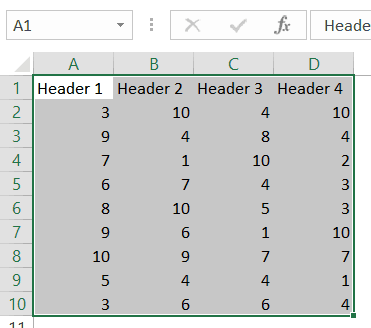
But in case you have blank rows/columns in your data, it will not select the ones after the blank rows/columns. In the image below, the CurrentRegion code selects data till row 10 as row 11 is blank.
![]()
In such cases, you may want to use the UsedRange property of the Worksheet Object.
Select Using UsedRange Property
UsedRange allows you to refer to any cells that have been changed.
So the below code would select all the used cells in the active sheet.
Note that in case you have a far-off cell that has been used, it would be considered by the above code and all the cells till that used cell would be selected.
Select Using the End Property
Now, this part is really useful.
The End property allows you to select the last filled cell. This allows you to mimic the effect of Control Down/Up arrow key or Control Right/Left keys.
Let’s try and understand this using an example.
Suppose you have a dataset as shown below and you want to quickly select the last filled cells in column A.
The problem here is that data can change and you don’t know how many cells are filled. If you have to do this using keyboard, you can select cell A1, and then use Control + Down arrow key, and it will select the last filled cell in the column.
Now let’s see how to do this using VBA. This technique comes in handy when you want to quickly jump to the last filled cell in a variably-sized column
The above code would jump to the last filled cell in column A.
Similarly, you can use the End(xlToRight) to jump to the last filled cell in a row.
Now, what if you want to select the entire column instead of jumping to the last filled cell.
You can do that using the code below:
In the above code, we have used the first and the last reference of the cell that we need to select. No matter how many filled cells are there, the above code will select all.
Remember the example above where we selected the range A1:D20 by using the following line of code:
Here A1 was the top-left cell and D20 was the bottom-right cell in the range. We can use the same logic in selecting variably sized ranges. But since we don’t know the exact address of the bottom-right cell, we used the End property to get it.
In Range(“A1”, Range(“A1”).End(xlDown)), “A1” refers to the first cell and Range(“A1”).End(xlDown) refers to the last cell. Since we have provided both the references, the Select method selects all the cells between these two references.
Similarly, you can also select an entire data set that has multiple rows and columns.
The below code would select all the filled rows/columns starting from cell A1.
In the above code, we have used Range(“A1”).End(xlDown).End(xlToRight) to get the reference of the bottom-right filled cell of the dataset.
Difference between Using CurrentRegion and End
If you’re wondering why use the End property to select the filled range when we have the CurrentRegion property, let me tell you the difference.
With End property, you can specify the start cell. For example, if you have your data in A1:D20, but the first row are headers, you can use the End property to select the data without the headers (using the code below).
But the CurrentRegion would automatically select the entire dataset, including the headers.
So far in this tutorial, we have seen how to refer to a range of cells using different ways.
Now let’s see some ways where we can actually use these techniques to get some work done.
Copy Cells / Ranges Using VBA
As I mentioned at the beginning of this tutorial, selecting a cell is not necessary to perform actions on it. You will see in this section how to copy cells and ranges without even selecting these.
Let’s start with a simple example.
Copying Single Cell
If you want to copy cell A1 and paste it into cell D1, the below code would do it.
Note that the copy method of the range object copies the cell (just like Control +C) and pastes it in the specified destination.
In the above example code, the destination is specified in the same line where you use the Copy method. If you want to make your code even more readable, you can use the below code:
The above codes will copy and paste the value as well as formatting/formulas in it.
As you might have already noticed, the above code copies the cell without selecting it. No matter where you’re on the worksheet, the code will copy cell A1 and paste it on D1.
Also, note that the above code would overwrite any existing code in cell D2. If you want Excel to let you know if there is already something in cell D1 without overwriting it, you can use the code below.
Copying a Fix Sized Range
If you want to copy A1:D20 in J1:M20, you can use the below code:
In the destination cell, you just need to specify the address of the top-left cell. The code would automatically copy the exact copied range into the destination.
You can use the same construct to copy data from one sheet to the other.
The below code would copy A1:D20 from the active sheet to Sheet2.
The above copies the data from the active sheet. So make sure the sheet that has the data is the active sheet before running the code. To be safe, you can also specify the worksheet’s name while copying the data.
The good thing about the above code is that no matter which sheet is active, it will always copy the data from Sheet1 and paste it in Sheet2.
You can also copy a named range by using its name instead of the reference.
For example, if you have a named range called ‘SalesData’, you can use the below code to copy this data to Sheet2.
If the scope of the named range is the entire workbook, you don’t need to be on the sheet that has the named range to run this code. Since the named range is scoped for the workbook, you can access it from any sheet using this code.
If you have a table with the name Table1, you can use the below code to copy it to Sheet2.
You can also copy a range to another Workbook.
In the following example, I copy the Excel table (Table1), into the Book2 workbook.
This code would work only if the Workbook is already open.
Copying a Variable Sized Range
One way to copy variable sized ranges is to convert these into named ranges or Excel Table and the use the codes as shown in the previous section.
But if you can’t do that, you can use the CurrentRegion or the End property of the range object.
The below code would copy the current region in the active sheet and paste it in Sheet2.
If you want to copy the first column of your data set till the last filled cell and paste it in Sheet2, you can use the below code:
If you want to copy the rows as well as columns, you can use the below code:
Note that all these codes don’t select the cells while getting executed. In general, you will find only a handful of cases where you actually need to select a cell/range before working on it.
Assigning Ranges to Object Variables
So far, we have been using the full address of the cells (such as Workbooks(“Book2.xlsx”).Worksheets(“Sheet1”).Range(“A1”)).
To make your code more manageable, you can assign these ranges to object variables and then use those variables.
For example, in the below code, I have assigned the source and destination range to object variables and then used these variables to copy data from one range to the other.
We start by declaring the variables as Range objects. Then we assign the range to these variables using the Set statement. Once the range has been assigned to the variable, you can simply use the variable.
Enter Data in the Next Empty Cell (Using Input Box)
You can use the Input boxes to allow the user to enter the data.
For example, suppose you have the data set below and you want to enter the sales record, you can use the input box in VBA. Using a code, we can make sure that it fills the data in the next blank row.
The above code uses the VBA Input box to get the inputs from the user, and then enters the inputs into the specified cells.
Note that we didn’t use exact cell references. Instead, we have used the End and Offset property to find the last empty cell and fill the data in it.
This code is far from usable. For example, if you enter a text string when the input box asks for quantity or amount, you will notice that Excel allows it. You can use an If condition to check whether the value is numeric or not and then allow it accordingly.
Looping Through Cells / Ranges
So far we can have seen how to select, copy, and enter the data in cells and ranges.
In this section, we will see how to loop through a set of cells/rows/columns in a range. This could be useful when you want to analyze each cell and perform some action based on it.
For example, if you want to highlight every third row in the selection, then you need to loop through and check for the row number. Similarly, if you want to highlight all the negative cells by changing the font color to red, you need to loop through and analyze each cell’s value.
Here is the code that will loop through the rows in the selected cells and highlight alternate rows.
The above code uses the MOD function to check the row number in the selection. If the row number is even, it gets highlighted in cyan color.
Here is another example where the code goes through each cell and highlights the cells that have a negative value in it.
Note that you can do the same thing using Conditional Formatting (which is dynamic and a better way to do this). This example is only for the purpose of showing you how looping works with cells and ranges in VBA.
Where to Put the VBA Code
Wondering where the VBA code goes in your Excel workbook?
Excel has a VBA backend called the VBA editor. You need to copy and paste the code in the VB Editor module code window.
Here are the steps to do this:
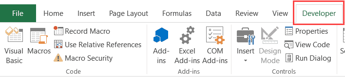
- Go to the Developer tab.

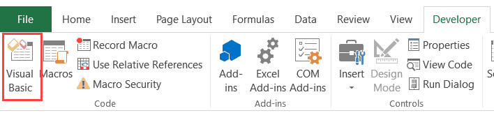
- Click on the Visual Basic option. This will open the VB editor in the backend.
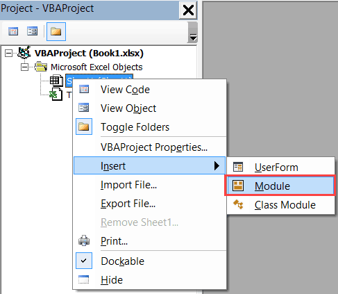
- In the Project Explorer pane in the VB Editor, right-click on any object for the workbook in which you want to insert the code. If you don’t see the Project Explorer, go to the View tab and click on Project Explorer.
- Go to Insert and click on Module. This will insert a module object for your workbook.
- Copy and paste the code in the module window.
You May Also Like the Following Excel Tutorials:
Источник
In this chapter you will learn how to change all the cells in the active sheet to values using VBA in Microsoft Excel.
Let’s take an example and understand how we write the VBA code for change the cells value in Active sheet.
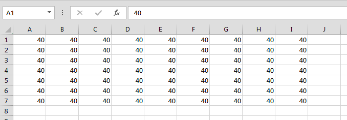
How to change all the cells value in the Active sheet?
We have data in Excel, in which we want the replace all the cells value with only a cell value.
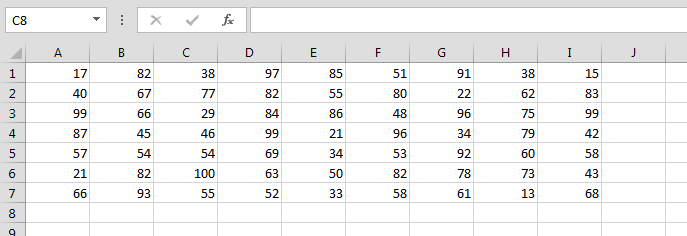
Follow below given steps:-
- Press Alt+F11 key to open the Visual Basic Application
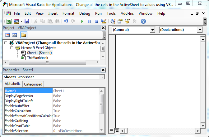
- In VBAProject Double click on Sheet 1
- Enter the below given VBA Code
Sub Values_1()

With ActiveSheet.UsedRange

Range("A1:I7").Value = Range("A2").Value

End With

End Sub
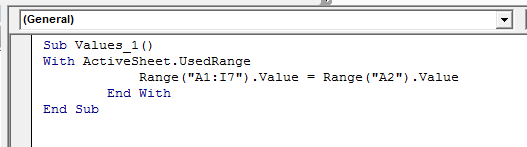
- To run the code press F5 key
- Cell A2 value will get update in the define range
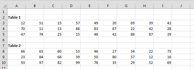
How the change the value from first table to second table?
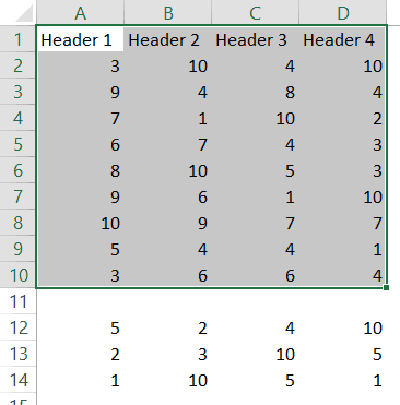
We have 2 tables, 1st table’s range is A3:I5, and 2nd table range is A8:I10. We want to replace the value of 1st table with the value of 2 table in the active sheet.
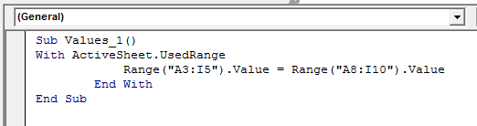
To change the value follow below given steps and code:-
- Open the Visual Basic Application
- Enter the below code:-
Sub Values_1()

With ActiveSheet.UsedRange

Range("A3:I5").Value = Range("A8:I10").Value

End With

End Sub
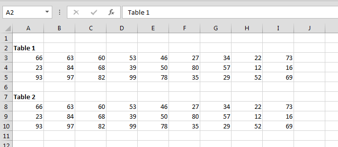
- Run the code by pressing F5
- Values will get updated
![]()
If you liked our blogs, share it with your friends on Facebook. And also you can follow us on Twitter and Facebook.
We would love to hear from you, do let us know how we can improve, complement or innovate our work and make it better for you. Write us at info@exceltip.com
In this Article
- Set Cell Value
- Range.Value & Cells.Value
- Set Multiple Cells’ Values at Once
- Set Cell Value – Text
- Set Cell Value – Variable
- Get Cell Value
- Get ActiveCell Value
- Assign Cell Value to Variable
- Other Cell Value Examples
- Copy Cell Value
- Compare Cell Values
This tutorial will teach you how to interact with Cell Values using VBA.
Set Cell Value
To set a Cell Value, use the Value property of the Range or Cells object.
Range.Value & Cells.Value
There are two ways to reference cell(s) in VBA:
- Range Object – Range(“A2”).Value
- Cells Object – Cells(2,1).Value
The Range object allows you to reference a cell using the standard “A1” notation.
This will set the range A2’s value = 1:
Range("A2").Value = 1The Cells object allows you to reference a cell by it’s row number and column number.
This will set range A2’s value = 1:
Cells(2,1).Value = 1Notice that you enter the row number first:
Cells(Row_num, Col_num)Set Multiple Cells’ Values at Once
Instead of referencing a single cell, you can reference a range of cells and change all of the cell values at once:
Range("A2:A5").Value = 1Set Cell Value – Text
In the above examples, we set the cell value equal to a number (1). Instead, you can set the cell value equal to a string of text. In VBA, all text must be surrounded by quotations:
Range("A2").Value = "Text"If you don’t surround the text with quotations, VBA will think you referencing a variable…
Set Cell Value – Variable
You can also set a cell value equal to a variable
Dim strText as String
strText = "String of Text"

Range("A2").Value = strText
Get Cell Value
You can get cell values using the same Value property that we used above.
VBA Coding Made Easy
Stop searching for VBA code online. Learn more about AutoMacro — A VBA Code Builder that allows beginners to code procedures from scratch with minimal coding knowledge and with many time-saving features for all users!

Learn More
Get ActiveCell Value
To get the ActiveCell value and display it in a message box:
MsgBox ActiveCell.ValueAssign Cell Value to Variable
To get a cell value and assign it to a variable:
Dim var as Variant

var = Range("A1").Value
Here we used a variable of type Variant. Variant variables can accept any type of values. Instead, you could use a String variable type:
Dim var as String

var = Range("A1").Value
A String variable type will accept numerical values, but it will store the numbers as text.
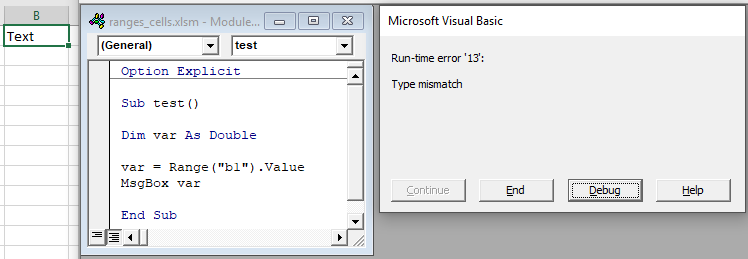
If you know your cell value will be numerical, you could use a Double variable type (Double variables can store decimal values):
Dim var as Double

var = Range("A1").Value
However, if you attempt to store a cell value containing text in a double variable, you will receive an type mismatch error:
Other Cell Value Examples
VBA Programming | Code Generator does work for you!
Copy Cell Value
It’s easy to set a cell value equal to another cell value (or “Copy” a cell value):
Range("A1").Value = Range("B1").ValueYou can even do this with ranges of cells (the ranges must be the same size):
Range("A1:A5").Value = Range("B1:B5").ValueCompare Cell Values
You can compare cell values using the standard comparison operators.
Test if cell values are equal:
MsgBox Range("A1").Value = Range("B1").ValueWill return TRUE if cell values are equal. Otherwise FALSE.
You can also create an If Statement to compare cell values:
If Range("A1").Value > Range("B1").Value Then

  Range("C1").Value = "Greater Than"

Elseif Range("A1").Value = Range("B1").Value Then

  Range("C1").Value = "Equal"

Else

  Range("C1").Value = "Less Than"

End If
You can compare text in the same way (Remember that VBA is Case Sensitive)
When working with Excel, most of your time is spent in the worksheet area – dealing with cells and ranges.
And if you want to automate your work in Excel using VBA, you need to know how to work with cells and ranges using VBA.
There are a lot of different things you can do with ranges in VBA (such as select, copy, move, edit, etc.).
So to cover this topic, I will break this tutorial into sections and show you how to work with cells and ranges in Excel VBA using examples.
Let’s get started.
All the codes I mention in this tutorial need to be placed in the VB Editor. Go to the ‘Where to Put the VBA Code‘ section to know how it works.
If you’re interested in learning VBA the easy way, check out my Online Excel VBA Training.
Selecting a Cell / Range in Excel using VBA
To work with cells and ranges in Excel using VBA, you don’t need to select it.
In most of the cases, you are better off not selecting cells or ranges (as we will see).
Despite that, it’s important you go through this section and understand how it works. This will be crucial in your VBA learning and a lot of concepts covered here will be used throughout this tutorial.
So let’s start with a very simple example.
Selecting a Single Cell Using VBA
If you want to select a single cell in the active sheet (say A1), then you can use the below code:
Sub SelectCell()
Range("A1").Select
End Sub
The above code has the mandatory ‘Sub’ and ‘End Sub’ part, and a line of code that selects cell A1.
Range(“A1”) tells VBA the address of the cell that we want to refer to.
Select is a method of the Range object and selects the cells/range specified in the Range object. The cell references need to be enclosed in double quotes.
This code would show an error in case a chart sheet is an active sheet. A chart sheet contains charts and is not widely used. Since it doesn’t have cells/ranges in it, the above code can’t select it and would end up showing an error.
Note that since you want to select the cell in the active sheet, you just need to specify the cell address.
But if you want to select the cell in another sheet (let’s say Sheet2), you need to first activate Sheet2 and then select the cell in it.
Sub SelectCell()
Worksheets("Sheet2").Activate
Range("A1").Select
End Sub
Similarly, you can also activate a workbook, then activate a specific worksheet in it, and then select a cell.
Sub SelectCell()
Workbooks("Book2.xlsx").Worksheets("Sheet2").Activate
Range("A1").Select
End Sub
Note that when you refer to workbooks, you need to use the full name along with the file extension (.xlsx in the above code). In case the workbook has never been saved, you don’t need to use the file extension.
Now, these examples are not very useful, but you will see later in this tutorial how we can use the same concepts to copy and paste cells in Excel (using VBA).
Just as we select a cell, we can also select a range.
In case of a range, it could be a fixed size range or a variable size range.
In a fixed size range, you would know how big the range is and you can use the exact size in your VBA code. But with a variable-sized range, you have no idea how big the range is and you need to use a little bit of VBA magic.
Let’s see how to do this.
Selecting a Fix Sized Range
Here is the code that will select the range A1:D20.
Sub SelectRange()
Range("A1:D20").Select
End Sub
Another way of doing this is using the below code:
Sub SelectRange()
Range("A1", "D20").Select
End Sub
The above code takes the top-left cell address (A1) and the bottom-right cell address (D20) and selects the entire range. This technique becomes useful when you’re working with variably sized ranges (as we will see when the End property is covered later in this tutorial).
If you want the selection to happen in a different workbook or a different worksheet, then you need to tell VBA the exact names of these objects.
For example, the below code would select the range A1:D20 in Sheet2 worksheet in the Book2 workbook.
Sub SelectRange()
Workbooks("Book2.xlsx").Worksheets("Sheet1").Activate
Range("A1:D20").Select
End Sub
Now, what if you don’t know how many rows are there. What if you want to select all the cells that have a value in it.
In these cases, you need to use the methods shown in the next section (on selecting variably sized range).
Selecting a Variably Sized Range
There are different ways you can select a range of cells. The method you choose would depend on how the data is structured.
In this section, I will cover some useful techniques that are really useful when you work with ranges in VBA.
Select Using CurrentRange Property
In cases where you don’t know how many rows/columns have the data, you can use the CurrentRange property of the Range object.
The CurrentRange property covers all the contiguous filled cells in a data range.
Below is the code that will select the current region that holds cell A1.
Sub SelectCurrentRegion()
Range("A1").CurrentRegion.Select
End Sub
The above method is good when you have all data as a table without any blank rows/columns in it.
But in case you have blank rows/columns in your data, it will not select the ones after the blank rows/columns. In the image below, the CurrentRegion code selects data till row 10 as row 11 is blank.
In such cases, you may want to use the UsedRange property of the Worksheet Object.
Select Using UsedRange Property
UsedRange allows you to refer to any cells that have been changed.
So the below code would select all the used cells in the active sheet.
Sub SelectUsedRegion()
ActiveSheet.UsedRange.Select
End Sub
Note that in case you have a far-off cell that has been used, it would be considered by the above code and all the cells till that used cell would be selected.
Select Using the End Property
Now, this part is really useful.
The End property allows you to select the last filled cell. This allows you to mimic the effect of Control Down/Up arrow key or Control Right/Left keys.
Let’s try and understand this using an example.
Suppose you have a dataset as shown below and you want to quickly select the last filled cells in column A.
The problem here is that data can change and you don’t know how many cells are filled. If you have to do this using keyboard, you can select cell A1, and then use Control + Down arrow key, and it will select the last filled cell in the column.
Now let’s see how to do this using VBA. This technique comes in handy when you want to quickly jump to the last filled cell in a variably-sized column
Sub GoToLastFilledCell()
Range("A1").End(xlDown).Select
End Sub
The above code would jump to the last filled cell in column A.
Similarly, you can use the End(xlToRight) to jump to the last filled cell in a row.
Sub GoToLastFilledCell()
Range("A1").End(xlToRight).Select
End Sub
Now, what if you want to select the entire column instead of jumping to the last filled cell.
You can do that using the code below:
Sub SelectFilledCells()
Range("A1", Range("A1").End(xlDown)).Select
End Sub
In the above code, we have used the first and the last reference of the cell that we need to select. No matter how many filled cells are there, the above code will select all.
Remember the example above where we selected the range A1:D20 by using the following line of code:
Range(“A1″,”D20”)
Here A1 was the top-left cell and D20 was the bottom-right cell in the range. We can use the same logic in selecting variably sized ranges. But since we don’t know the exact address of the bottom-right cell, we used the End property to get it.
In Range(“A1”, Range(“A1”).End(xlDown)), “A1” refers to the first cell and Range(“A1”).End(xlDown) refers to the last cell. Since we have provided both the references, the Select method selects all the cells between these two references.
Similarly, you can also select an entire data set that has multiple rows and columns.
The below code would select all the filled rows/columns starting from cell A1.
Sub SelectFilledCells()
Range("A1", Range("A1").End(xlDown).End(xlToRight)).Select
End Sub
In the above code, we have used Range(“A1”).End(xlDown).End(xlToRight) to get the reference of the bottom-right filled cell of the dataset.
Difference between Using CurrentRegion and End
If you’re wondering why use the End property to select the filled range when we have the CurrentRegion property, let me tell you the difference.
With End property, you can specify the start cell. For example, if you have your data in A1:D20, but the first row are headers, you can use the End property to select the data without the headers (using the code below).
Sub SelectFilledCells()
Range("A2", Range("A2").End(xlDown).End(xlToRight)).Select
End Sub
But the CurrentRegion would automatically select the entire dataset, including the headers.
So far in this tutorial, we have seen how to refer to a range of cells using different ways.
Now let’s see some ways where we can actually use these techniques to get some work done.
Copy Cells / Ranges Using VBA
As I mentioned at the beginning of this tutorial, selecting a cell is not necessary to perform actions on it. You will see in this section how to copy cells and ranges without even selecting these.
Let’s start with a simple example.
Copying Single Cell
If you want to copy cell A1 and paste it into cell D1, the below code would do it.
Sub CopyCell()
Range("A1").Copy Range("D1")
End Sub
Note that the copy method of the range object copies the cell (just like Control +C) and pastes it in the specified destination.
In the above example code, the destination is specified in the same line where you use the Copy method. If you want to make your code even more readable, you can use the below code:
Sub CopyCell()
Range("A1").Copy Destination:=Range("D1")
End Sub
The above codes will copy and paste the value as well as formatting/formulas in it.
As you might have already noticed, the above code copies the cell without selecting it. No matter where you’re on the worksheet, the code will copy cell A1 and paste it on D1.
Also, note that the above code would overwrite any existing code in cell D2. If you want Excel to let you know if there is already something in cell D1 without overwriting it, you can use the code below.
Sub CopyCell()
If Range("D1") <> "" Then
Response = MsgBox("Do you want to overwrite the existing data", vbYesNo)
End If
If Response = vbYes Then
Range("A1").Copy Range("D1")
End If
End Sub
Copying a Fix Sized Range
If you want to copy A1:D20 in J1:M20, you can use the below code:
Sub CopyRange()
Range("A1:D20").Copy Range("J1")
End Sub
In the destination cell, you just need to specify the address of the top-left cell. The code would automatically copy the exact copied range into the destination.
You can use the same construct to copy data from one sheet to the other.
The below code would copy A1:D20 from the active sheet to Sheet2.
Sub CopyRange()
Range("A1:D20").Copy Worksheets("Sheet2").Range("A1")
End Sub
The above copies the data from the active sheet. So make sure the sheet that has the data is the active sheet before running the code. To be safe, you can also specify the worksheet’s name while copying the data.
Sub CopyRange()
Worksheets("Sheet1").Range("A1:D20").Copy Worksheets("Sheet2").Range("A1")
End Sub
The good thing about the above code is that no matter which sheet is active, it will always copy the data from Sheet1 and paste it in Sheet2.
You can also copy a named range by using its name instead of the reference.
For example, if you have a named range called ‘SalesData’, you can use the below code to copy this data to Sheet2.
Sub CopyRange()
Range("SalesData").Copy Worksheets("Sheet2").Range("A1")
End Sub
If the scope of the named range is the entire workbook, you don’t need to be on the sheet that has the named range to run this code. Since the named range is scoped for the workbook, you can access it from any sheet using this code.
If you have a table with the name Table1, you can use the below code to copy it to Sheet2.
Sub CopyTable()
Range("Table1[#All]").Copy Worksheets("Sheet2").Range("A1")
End Sub
You can also copy a range to another Workbook.
In the following example, I copy the Excel table (Table1), into the Book2 workbook.
Sub CopyCurrentRegion()
Range("Table1[#All]").Copy Workbooks("Book2.xlsx").Worksheets("Sheet1").Range("A1")
End Sub
This code would work only if the Workbook is already open.
Copying a Variable Sized Range
One way to copy variable sized ranges is to convert these into named ranges or Excel Table and the use the codes as shown in the previous section.
But if you can’t do that, you can use the CurrentRegion or the End property of the range object.
The below code would copy the current region in the active sheet and paste it in Sheet2.
Sub CopyCurrentRegion()
Range("A1").CurrentRegion.Copy Worksheets("Sheet2").Range("A1")
End Sub
If you want to copy the first column of your data set till the last filled cell and paste it in Sheet2, you can use the below code:
Sub CopyCurrentRegion()
Range("A1", Range("A1").End(xlDown)).Copy Worksheets("Sheet2").Range("A1")
End Sub
If you want to copy the rows as well as columns, you can use the below code:
Sub CopyCurrentRegion()
Range("A1", Range("A1").End(xlDown).End(xlToRight)).Copy Worksheets("Sheet2").Range("A1")
End Sub
Note that all these codes don’t select the cells while getting executed. In general, you will find only a handful of cases where you actually need to select a cell/range before working on it.
Assigning Ranges to Object Variables
So far, we have been using the full address of the cells (such as Workbooks(“Book2.xlsx”).Worksheets(“Sheet1”).Range(“A1”)).
To make your code more manageable, you can assign these ranges to object variables and then use those variables.
For example, in the below code, I have assigned the source and destination range to object variables and then used these variables to copy data from one range to the other.
Sub CopyRange()
Dim SourceRange As Range
Dim DestinationRange As Range
Set SourceRange = Worksheets("Sheet1").Range("A1:D20")
Set DestinationRange = Worksheets("Sheet2").Range("A1")
SourceRange.Copy DestinationRange
End Sub
We start by declaring the variables as Range objects. Then we assign the range to these variables using the Set statement. Once the range has been assigned to the variable, you can simply use the variable.
Enter Data in the Next Empty Cell (Using Input Box)
You can use the Input boxes to allow the user to enter the data.
For example, suppose you have the data set below and you want to enter the sales record, you can use the input box in VBA. Using a code, we can make sure that it fills the data in the next blank row.
Sub EnterData()
Dim RefRange As Range
Set RefRange = Range("A1").End(xlDown).Offset(1, 0)
Set ProductCategory = RefRange.Offset(0, 1)
Set Quantity = RefRange.Offset(0, 2)
Set Amount = RefRange.Offset(0, 3)
RefRange.Value = RefRange.Offset(-1, 0).Value + 1
ProductCategory.Value = InputBox("Product Category")
Quantity.Value = InputBox("Quantity")
Amount.Value = InputBox("Amount")
End Sub
The above code uses the VBA Input box to get the inputs from the user, and then enters the inputs into the specified cells.
Note that we didn’t use exact cell references. Instead, we have used the End and Offset property to find the last empty cell and fill the data in it.
This code is far from usable. For example, if you enter a text string when the input box asks for quantity or amount, you will notice that Excel allows it. You can use an If condition to check whether the value is numeric or not and then allow it accordingly.
Looping Through Cells / Ranges
So far we can have seen how to select, copy, and enter the data in cells and ranges.
In this section, we will see how to loop through a set of cells/rows/columns in a range. This could be useful when you want to analyze each cell and perform some action based on it.
For example, if you want to highlight every third row in the selection, then you need to loop through and check for the row number. Similarly, if you want to highlight all the negative cells by changing the font color to red, you need to loop through and analyze each cell’s value.
Here is the code that will loop through the rows in the selected cells and highlight alternate rows.
Sub HighlightAlternateRows()
Dim Myrange As Range
Dim Myrow As Range
Set Myrange = Selection
For Each Myrow In Myrange.Rows
If Myrow.Row Mod 2 = 0 Then
Myrow.Interior.Color = vbCyan
End If
Next Myrow
End Sub
The above code uses the MOD function to check the row number in the selection. If the row number is even, it gets highlighted in cyan color.
Here is another example where the code goes through each cell and highlights the cells that have a negative value in it.
Sub HighlightAlternateRows()
Dim Myrange As Range
Dim Mycell As Range
Set Myrange = Selection
For Each Mycell In Myrange
If Mycell < 0 Then
Mycell.Interior.Color = vbRed
End If
Next Mycell
End Sub
Note that you can do the same thing using Conditional Formatting (which is dynamic and a better way to do this). This example is only for the purpose of showing you how looping works with cells and ranges in VBA.
Where to Put the VBA Code
Wondering where the VBA code goes in your Excel workbook?
Excel has a VBA backend called the VBA editor. You need to copy and paste the code in the VB Editor module code window.
Here are the steps to do this:
- Go to the Developer tab.

- Click on the Visual Basic option. This will open the VB editor in the backend.
- In the Project Explorer pane in the VB Editor, right-click on any object for the workbook in which you want to insert the code. If you don’t see the Project Explorer, go to the View tab and click on Project Explorer.
- Go to Insert and click on Module. This will insert a module object for your workbook.

- Copy and paste the code in the module window.

You May Also Like the Following Excel Tutorials:
- Working with Worksheets using VBA.
- Working with Workbooks using VBA.
- Creating User-Defined Functions in Excel.
- For Next Loop in Excel VBA – A Beginner’s Guide with Examples.
- How to Use Excel VBA InStr Function (with practical EXAMPLES).
- Excel VBA Msgbox.
- How to Record a Macro in Excel.
- How to Run a Macro in Excel.
- How to Create an Add-in in Excel.
- Excel Personal Macro Workbook | Save & Use Macros in All Workbooks.
- Excel VBA Events – An Easy (and Complete) Guide.
- Excel VBA Error Handling.
- How to Sort Data in Excel using VBA (A Step-by-Step Guide).
- 24 Useful Excel Macro Examples for VBA Beginners (Ready-to-use).
Formatting Cells Number
General
Range("A1").NumberFormat = "General"Number
Range("A1").NumberFormat = "0.00"Currency
Range("A1").NumberFormat = "$#,##0.00"Accounting
Range("A1").NumberFormat = "_($* #,##0.00_);_($* (#,##0.00);_($* ""-""??_);_(@_)"Date
Range("A1").NumberFormat = "yyyy-mm-dd;@"Time
Range("A1").NumberFormat = "h:mm:ss AM/PM;@"Percentage
Range("A1").NumberFormat = "0.00%"Fraction
Range("A1").NumberFormat = "# ?/?"Scientific
Range("A1").NumberFormat = "0.00E+00"Text
Range("A1").NumberFormat = "@"Special
Range("A1").NumberFormat = "00000"Custom
Range("A1").NumberFormat = "$#,##0.00_);[Red]($#,##0.00)"Formatting Cells Alignment
Text Alignment
Horizontal
The value of this property can be set to one of the constants: xlGeneral, xlCenter, xlDistributed, xlJustify, xlLeft, xlRight.
The following code sets the horizontal alignment of cell A1 to center.
Range("A1").HorizontalAlignment = xlCenterVertical
The value of this property can be set to one of the constants: xlBottom, xlCenter, xlDistributed, xlJustify, xlTop.
The following code sets the vertical alignment of cell A1 to bottom.
Range("A1").VerticalAlignment = xlBottomText Control
Wrap Text
This example formats cell A1 so that the text wraps within the cell.
Range("A1").WrapText = TrueShrink To Fit
This example causes text in row one to automatically shrink to fit in the available column width.
Rows(1).ShrinkToFit = TrueMerge Cells
This example merge range A1:A4 to a large one.
Range("A1:A4").MergeCells = TrueRight-to-left
Text direction
The value of this property can be set to one of the constants: xlRTL (right-to-left), xlLTR (left-to-right), or xlContext (context).
The following code example sets the reading order of cell A1 to xlRTL (right-to-left).
Range("A1").ReadingOrder = xlRTLOrientation
The value of this property can be set to an integer value from –90 to 90 degrees or to one of the following constants: xlDownward, xlHorizontal, xlUpward, xlVertical.
The following code example sets the orientation of cell A1 to xlHorizontal.
Range("A1").Orientation = xlHorizontalFont
Font Name
The value of this property can be set to one of the fonts: Calibri, Times new Roman, Arial…
The following code sets the font name of range A1:A5 to Calibri.
Range("A1:A5").Font.Name = "Calibri"Font Style
The value of this property can be set to one of the constants: Regular, Bold, Italic, Bold Italic.
The following code sets the font style of range A1:A5 to Italic.
Range("A1:A5").Font.FontStyle = "Italic"Font Size
The value of this property can be set to an integer value from 1 to 409.
The following code sets the font size of cell A1 to 14.
Range("A1").Font.Size = 14Underline
The value of this property can be set to one of the constants: xlUnderlineStyleNone, xlUnderlineStyleSingle, xlUnderlineStyleDouble, xlUnderlineStyleSingleAccounting, xlUnderlineStyleDoubleAccounting.
The following code sets the font of cell A1 to xlUnderlineStyleDouble (double underline).
Range("A1").Font.Underline = xlUnderlineStyleDoubleFont Color
The value of this property can be set to one of the standard colors: vbBlack, vbRed, vbGreen, vbYellow, vbBlue, vbMagenta, vbCyan, vbWhite or an integer value from 0 to 16,581,375.
To assist you with specifying the color of anything, the VBA is equipped with a function named RGB. Its syntax is:
Function RGB(RedValue As Byte, GreenValue As Byte, BlueValue As Byte) As longThis function takes three arguments and each must hold a value between 0 and 255. The first argument represents the ratio of red of the color. The second argument represents the green ratio of the color. The last argument represents the blue of the color. After the function has been called, it produces a number whose maximum value can be 255 * 255 * 255 = 16,581,375, which represents a color.
The following code sets the font color of cell A1 to vbBlack (Black).
Range("A1").Font.Color = vbBlackThe following code sets the font color of cell A1 to 0 (Black).
Range("A1").Font.Color = 0The following code sets the font color of cell A1 to RGB(0, 0, 0) (Black).
Range("A1").Font.Color = RGB(0, 0, 0)Font Effects
Strikethrough
True if the font is struck through with a horizontal line.
The following code sets the font of cell A1 to strikethrough.
Range("A1").Font.Strikethrough = TrueSubscript
True if the font is formatted as subscript. False by default.
The following code sets the font of cell A1 to Subscript.
Range("A1").Font.Subscript = TrueSuperscript
True if the font is formatted as superscript; False by default.
The following code sets the font of cell A1 to Superscript.
Range("A1").Font.Superscript = TrueBorder
Border Index
Using VBA you can choose to create borders for the different edges of a range of cells:
- xlDiagonalDown (Border running from the upper left-hand corner to the lower right of each cell in the range).
- xlDiagonalUp (Border running from the lower left-hand corner to the upper right of each cell in the range).
- xlEdgeBottom (Border at the bottom of the range).
- xlEdgeLeft (Border at the left-hand edge of the range).
- xlEdgeRight (Border at the right-hand edge of the range).
- xlEdgeTop (Border at the top of the range).
- xlInsideHorizontal (Horizontal borders for all cells in the range except borders on the outside of the range).
- xlInsideVertical (Vertical borders for all the cells in the range except borders on the outside of the range).
Line Style
The value of this property can be set to one of the constants: xlContinuous (Continuous line), xlDash (Dashed line), xlDashDot (Alternating dashes and dots), xlDashDotDot (Dash followed by two dots), xlDot (Dotted line), xlDouble (Double line), xlLineStyleNone (No line), xlSlantDashDot (Slanted dashes).
The following code example sets the border on the bottom edge of cell A1 with continuous line.
Range("A1").Borders(xlEdgeBottom).LineStyle = xlContinuousThe following code example removes the border on the bottom edge of cell A1.
Range("A1").Borders(xlEdgeBottom).LineStyle = xlNoneLine Thickness
The value of this property can be set to one of the constants: xlHairline (Hairline, thinnest border), xlMedium (Medium), xlThick (Thick, widest border), xlThin (Thin).
The following code example sets the thickness of the border created to xlThin (Thin).
Range("A1").Borders(xlEdgeBottom).Weight = xlThinLine Color
The value of this property can be set to one of the standard colors: vbBlack, vbRed, vbGreen, vbYellow, vbBlue, vbMagenta, vbCyan, vbWhite or an integer value from 0 to 16,581,375.
The following code example sets the color of the border on the bottom edge to green.
Range("A1").Borders(xlEdgeBottom).Color = vbGreenYou can also use the RGB function to create a color value.
The following example sets the color of the bottom border of cell A1 with RGB fuction.
Range("A1").Borders(xlEdgeBottom).Color = RGB(255, 0, 0)Fill
Pattern Style
The value of this property can be set to one of the constants:
- xlPatternAutomatic (Excel controls the pattern.)
- xlPatternChecker (Checkerboard.)
- xlPatternCrissCross (Criss-cross lines.)
- xlPatternDown (Dark diagonal lines running from the upper left to the lower right.)
- xlPatternGray16 (16% gray.)
- xlPatternGray25 (25% gray.)
- xlPatternGray50 (50% gray.)
- xlPatternGray75 (75% gray.)
- xlPatternGray8 (8% gray.)
- xlPatternGrid (Grid.)
- xlPatternHorizontal (Dark horizontal lines.)
- xlPatternLightDown (Light diagonal lines running from the upper left to the lower right.)
- xlPatternLightHorizontal (Light horizontal lines.)
- xlPatternLightUp (Light diagonal lines running from the lower left to the upper right.)
- xlPatternLightVertical (Light vertical bars.)
- xlPatternNone (No pattern.)
- xlPatternSemiGray75 (75% dark moiré.)
- xlPatternSolid (Solid color.)
- xlPatternUp (Dark diagonal lines running from the lower left to the upper right.)
Protection
Locking Cells
This property returns True if the object is locked, False if the object can be modified when the sheet is protected, or Null if the specified range contains both locked and unlocked cells.
The following code example unlocks cells A1:B22 on Sheet1 so that they can be modified when the sheet is protected.
Worksheets("Sheet1").Range("A1:B22").Locked = False
Worksheets("Sheet1").Protect
Hiding Formulas
This property returns True if the formula will be hidden when the worksheet is protected, Null if the specified range contains some cells with FormulaHidden equal to True and some cells with FormulaHidden equal to False.
Don’t confuse this property with the Hidden property. The formula will not be hidden if the workbook is protected and the worksheet is not, but only if the worksheet is protected.
The following code example hides the formulas in cells A1 and C1 on Sheet1 when the worksheet is protected.
Worksheets("Sheet1").Range("A1:C1").FormulaHidden = True