
Содержание
- Объект Style (Excel)
- Замечания
- Пример
- Методы
- Свойства
- См. также
- Поддержка и обратная связь
- VBA Format Cells
- Formatting Cells
- AddIndent
- Borders
- FormulaHidden
- HorizontalAlignment
- VBA Coding Made Easy
- IndentLevel
- Interior
- Locked
- MergeCells
- NumberFormat
- NumberFormatLocal
- Orientation
- Parent
- ShrinkToFit
- VerticalAlignment
- WrapText
- VBA Code Examples Add-in
- Styles in Excel
- Content
- Introduction
- How styles work
- Creating styles
- Applying styles
- Deviate from a style
- Tips for using styles
- Managing styles
- Using styles
- Use functional sets of styles
- VBA examples and tools
- Find cells with a certain style
- Creating a list of styles
- Clear all formatting of cells and re-apply their styles
- Replace one style with another
- Removing formating from an Excel Table
- Conclusion
- Comments
Объект Style (Excel)
Представляет описание стиля для диапазона.
Замечания
Объект Style содержит все атрибуты стиля (шрифт, числовой формат, выравнивание и т. д.) в качестве свойств. Существует несколько встроенных стилей, включая обычный, денежный и процент. Использование объекта Style — это быстрый и эффективный способ одновременного изменения нескольких свойств форматирования ячеек в нескольких ячейках.
Для объекта Workbook объект Style является членом коллекции Styles . Коллекция Styles содержит все определенные стили для книги.
Внешний вид ячейки можно изменить, изменив свойства стиля, примененные к ней. Однако помните, что изменение свойства стиля влияет на все ячейки, уже отформатированные с помощью этого стиля.
Стили сортируются в алфавитном порядке по имени стиля. Номер индекса стиля обозначает позицию указанного стиля в отсортованном списке имен стилей. Styles(1) — это первый стиль в алфавитном списке и Styles(Styles.Count) последний стиль в списке.
Дополнительные сведения о создании и изменении стиля см. в разделе Объект Styles .
Пример
Используйте свойство Style , чтобы вернуть объект Style , используемый с объектом Range . В следующем примере стиль процент применяется к ячейкам A1:A10 на Листе1.
Используйте стили (index), где index — это номер или имя индекса стиля, чтобы вернуть один объект Style из коллекции стили книги. В следующем примере изменяется стиль «Обычный» для активной книги путем задания свойства «Полужирный» стиля.
Методы
Свойства
См. также
Поддержка и обратная связь
Есть вопросы или отзывы, касающиеся Office VBA или этой статьи? Руководство по другим способам получения поддержки и отправки отзывов см. в статье Поддержка Office VBA и обратная связь.
Источник
VBA Format Cells
In this Article
This tutorial will demonstrate how to format cells using VBA.
Formatting Cells
There are many formatting properties that can be set for a (range of) cells like this:
Let’s see them in alphabetical order:
AddIndent
By setting the value of this property to True the text will be automatically indented when the text alignment in the cell is set, either horizontally or vertically, to equal distribution (see HorizontalAlignment and VerticalAlignment).
Borders
You can set the border format of a cell. See here for more information about borders.
As an example you can set a red dashed line around cell B2 on Sheet 1 like this:
You can adjust the cell’s font format by setting the font name, style, size, color, adding underlines and or effects (strikethrough, sub- or superscript). See here for more information about cell fonts.
Here are some examples:
FormulaHidden
This property returns or sets a variant value that indicates if the formula will be hidden when the worksheet is protected. For example:
HorizontalAlignment
This property cell format property returns or sets a variant value that represents the horizontal alignment for the specified object. Returned or set constants can be: xlGeneral, xlCenter, xlDistributed, xlJustify, xlLeft, xlRight, xlFill, xlCenterAcrossSelection. For example:
VBA Coding Made Easy
Stop searching for VBA code online. Learn more about AutoMacro — A VBA Code Builder that allows beginners to code procedures from scratch with minimal coding knowledge and with many time-saving features for all users!

IndentLevel
It returns or sets an integer value between 0 and 15 that represents the indent level for the cell or range.
Interior
You can set or get returned information about the cell’s interior: its Color, ColorIndex, Pattern, PatternColor, PatternColorIndex, PatternThemeColor, PatternTintAndShade, ThemeColor, TintAndShade, like this:
Locked
This property returns True if the cell or range is locked, False if the object can be modified when the sheet is protected, or Null if the specified range contains both locked and unlocked cells. It can be used also for locking or unlocking cells.
This example unlocks cells A1:B2 on Sheet1 so that they can be modified when the sheet is protected.
MergeCells
Set this property to True if you need to merge a range. Its value gets True if a specified range contains merged cells. For example, if you need to merge the range of C5:D7, you can use this code:
NumberFormat
You can set the number format within the cell(s) to General, Number, Currency, Accounting, Date, Time, Percentage, Fraction, Scientific, Text, Special and Custom.
Here are the examples of scientific and percentage number formats:
NumberFormatLocal
This property returns or sets a variant value that represents the format code for the object as a string in the language of the user.
Orientation
You can set (or get returned) the text orientation within the cell(s) by this property. Its value can be one of these constants: xlDownward, xlHorizontal, xlUpward, xlVertical or an integer value from –90 to 90 degrees.
Parent
This is a read-only property that returns the parent object of a specified object.
ShrinkToFit
This property returns or sets a variant value that indicates if text automatically shrinks to fit in the available column width.
VerticalAlignment
This property cell format property returns or sets a variant value that represents the vertical alignment for the specified object. Returned or set constants can be: xlCenter, xlDistributed, xlJustify, xlBottom, xlTop. For example:
WrapText
This property returns True if text is wrapped in all cells within the specified range, False if text is not wrapped in all cells within the specified range, or Null if the specified range contains some cells that wrap text and other cells that don’t.
For example, if you have this range of cells: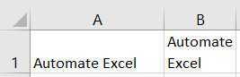
this code below will return Null in the Immediate Window:

VBA Code Examples Add-in
Easily access all of the code examples found on our site.
Simply navigate to the menu, click, and the code will be inserted directly into your module. .xlam add-in.
Источник
Styles in Excel
Content
Introduction
This article has also been published on Microsoft’s MSDN site:
This article explains how you can use styles to ease maintenance of your spreadsheet models.
Microsoft has made it very easy to dress up your worksheets with all sorts of fill patterns, borders and other frills. Because formatting of cells is often done in an ad-hoc manner, many spreadsheet pages look messy.
By consistently using cell styles (instead of changing parts of the cell’s formatting) you will be forced to think about the structure of your work. Religiously using styles may even force you to reconsider the overall structure of the entire spreadsheet model: The quality of the computational model itself may be positively affected.
I therefore consider Styles as being underused, underestimated and under exposed.
How styles work
A style is just a set of cell formatting settings which has been given a name. All cells to which a style has been applied look the same formatting-wise. When you change a part of a style, all cells to which that style has been applied change their formatting accordingly.
Use of styles takes some getting accustomed to, but may bring you great advantage. Imagine showing your nicely formatted sheet to your boss. Then your boss asks you if you could please change all input cells to having a light-yellow background fill, instead of a dark yellow one. For a large model, this may imply a huge amount of work. Would you have used styles, then it would have been a matter of seconds.
Styles are in fact an addition. Cell formatting is the sum of the applied style and all modifications to individual formatting elements on top of that style. What parts of the formatting options are included in a style is determined during the definition of the style (See screenshot below).
You access the style dialog from the Home Tab, Styles group, Cell Styles button:
Excel enables you to access the styles by clicking the dropdown next to the styles gallery. The screen to create a new style looks like this (if you click the New Cell Style option in the style gallery):
When you apply a style to a cell followed by another style, the end result will be an addition of the selected parts of both styles. What the end result of such an addition of styles will be, depends on which elements of both styles have been selected as being part of the style (this will be discussed later). Theoretically, this would have enabled us to use cascading styles, but unfortunately Excel does not keep a record of the order of applied styles. Only the last style is remembered. Also, styles can not be derived from other styles whilst maintaining a link to the parent style. Changes to the «original» style are not reflected in the «child» styles.
Creating styles
A convenient method to create a new style is by selecting a cell which has all formatting options in place which you want to incorporate in the new style. Select the cell and click the Home tab, click the New Cell Style button at the bottom of the Styles gallery.
The Styles dialog screen.
To create a new style, simply type its name in the box «Style name». By default, all formatting elements are checked. Remove the checkmarks for the formatting elements you want to omit from the style you are creating (The dialog shown above has the Number and Alignment elements turned off).
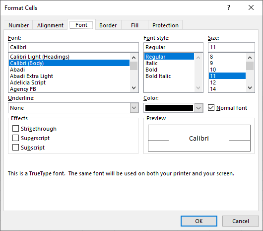
Use the «Modify. » button to adjust the elements to your needs. Excel will show the standard «Format cells » dialog screen:
The format cells dialog screen, as shown after clicking Modify. on the Style dialog.
Note, that the elements in the Style dialog are identical to the tabs on the Format Cells dialog.
Note: As soon as you change a formatting element on a tab that was not selected on the Style dialog, Excel will automatically check that element for you; it will become part of that style.
Note that the style dialog will update/add the style, but the style will not be applied to the selected cells.
Applying styles
To apply a style to a cell, you simply click the Home tab and in the Styles group you Expand the Cell Styles gallery and click a style.
Deviate from a style
If you have applied a style to a set of cells and you change a formatting element of one of those cells, then modifications to that particular element of the style will no longer be applied to the modified cell.
So after changing a font attribute (like Bold) of a cell, changing the font attributes of the style will update all cells, except the one you just modified:
Series of cells with one style, 1 cell deviates from that style.
You can restore the style of a cell simply by selecting the cell and choosing the style from the style gallery.
Tips for using styles
Managing styles
If you like to keep an overview of what styles are available in your file I’d advise you to add a special worksheet to your workbook. Put the names of the styles in column A and an example output in column B:
Table with styles in a worksheet
If you need to adjust a style, select the cell in column B and adjust the style settings from there.
Creating a new style based on an existing one is easy now: Just copy the applicable row and insert it anywhere in the table. Select the cell in column B of the newly inserted row and choose Home, Cell styles gallery, New Cell Style. Enter the name of the new style and click the Format button to change the style details. Don’t forget to update the Style name in column A too.
Using styles
I advise you to use styles as strictly as you can. Avoid modifying one formatting element of a cell with a style. Instead, consider if it is worth the effort to add a new style. If for instance you have a style for percentage with 2 decimal places and you have a cell which requires three, then add a style for that purpose. You can thank me later.
Adapting this method will likely trigger you to think about what cell styles your document will need. By doing this your Excel models will gradually improve. You’ll gain in consistency and loose the ad-hoc (often messy) formatting jungle.
Use functional sets of styles
By looking at your Excel model you will likely be able to categorise your workbook cells into various categories:
- Input cells
Cells that are the main input to your model - Parameter cells
Cells that contain constants for your model, such as boundaries. - Output cells
Cells in an area that is meant for output, such as printing or presenting the results of a calculation on screen. - Calculation cells
The cells where the actual calculation work is performed - Boundary cells
By shading otherwise empty cells you can easily make areas with differing functions stand out from other areas.
Consider creating styles for each of these cell functions, each (e.g.) having its own fill color. Don’t forget to make decisions on whether or not a style’s locked property needs to be on or off. If you use a system like this, it becomes very easy for you to maintain your file. Imagine how easy it now becomes to change a cell from an input to an output cell: you change its style. Done.
The little VBA routines shown below will greatly easy your work with styles. As an important side effect, these also show you how the style object works in VBA.
Find cells with a certain style
This routine find cells with a style containing «demo» in its name:
As soon as a cell is encountered with a style that matches that name filter, the code stops (Stop) and you can check out the cell in detail.
Creating a list of styles
This sub adds a table of your styles on a worksheet named «Config — Styles»:
Clear all formatting of cells and re-apply their styles
The code below removes all formatting of all cells and subsequently re-applies their style to them.
Watch out: if you have not adhered to using styles strictly, you may lose all formatting in your file.
Replace one style with another
The code below uses a list with two columns. The column on the left contains the names of existing styles. The column to its immediate right contains the names of the style you want to replace them with.
The code will run through the selected cells in the left column and check if the style name in the column to its right differs. If so, it will prompt you with the alternative name. Clicking OK will cause the code to update ALL cells to which the old style was applied to the new style. Before running this sub you need to select the cells in the left hand column.
Removing formating from an Excel Table
Suppose you have just converted a range to a table (see this article), but the range had some formatting set up such as background fills and borders. Tables allow you to format things like that automatically, but now your preexisting formatting messes up the table formatting. One way to overcome this is by changing the style of the cells in the table back to the Normal style. This however removes your number formats too. The little macro below fixes that by first making a copy of the normal style, setting its Number checkbox to false and then applying the new style without number format to the table. Finally it applies the tablestyle and deletes the temporary style:
Conclusion
There is a lot to gain by using styles in your Excel work. To name but a few:
- Consistent formatting of your models
- Ease of maintenance
- A strict use of styles leads to a structured way of working
- Less problems with your file (There is a limit on how many different cell formats Excel can handle).
With this article I have tried to give insight in the use of styles in Excel. If you have comments, suggestions or questions, please don’t hesitate to use the comment form below each page!
Showing last 8 comments of 128 in total (Show All Comments):
Comment by: Chris Greaves (2-5-2019 16:31:00) deeplink to this comment
Hi Jan Karel
Thanks for blnFindaStyle. I have «borrowed» a copy.
Too, I have posted a follow-up question on Eileen’s Lounge.
No need to post this here; I just wanted you to know that your name was being taken, but not in Vain.
Comment by: Jan Karel Pieterse (2-5-2019 17:16:00) deeplink to this comment
Comment by: Thaddeus Lesnik (9-8-2019 16:11:00) deeplink to this comment
I’d love to have a user menu box with two drop down lists, each populated with the list of styles.
The purpose of having two drop down boxes would be to select one style from the list then in listbox 1 then choose a different style from the list to replace it with using listbox 2. This would be useful if, for example, I have a style which got duplicated when I copy a sheet and the style intent is the same, but two slightly different name exist.
Comment by: Jan Karel Pieterse (9-8-2019 17:34:00) deeplink to this comment
You can use the routine called FixStyles to find out how to implement a part of what you need.
Comment by: Thaddeus Lesnik (12-8-2019 21:08:00) deeplink to this comment
For what it’s worth, here’s a clean summary of what the code became (can be placed completely in the Userform code or broken into modules and forms). Note to webmaster, I can share the modules and forms if that would be useful.
Sub UserForm_Initialize()
Dim oSt As Style
For Each oSt In ThisWorkbook.Styles
lstbxSource.AddItem oSt.Name
lstbxDest.AddItem oSt.Name
Next oSt
End Sub
Sub cmdChange_Click() ‘this is the userform button.
Dim strOldSt As String
Dim strNewSt As String
strOldSt = frmStyles.lstbxSource.Text
strNewSt = frmStyles.lstbxDest.Text
Call FixStyles(strOldSt, strNewSt)
‘Report on the Status of the Completion of the Process
MsgBox «Cell Style has been remapped!», vbInformation
End Sub
Sub FixStyles(strOldSt As String, strNewSt As String)
‘————————————————————————-
‘ Procedure : FixStyles
‘ Purpose : Replaces styles with the replacement style as defined by listboxes in a userform.
‘ Listbox 1 should contain the existing style, Listbox 2 the replacing style
‘————————————————————————-
Dim oWs As Worksheet
Dim oCell As Range
If strNewSt = «» Then Exit Sub
If strNewSt <> «» And strNewSt <> strOldSt Then
For Each oWs In ThisWorkbook.Worksheets
For Each oCell In oWs.UsedRange
If oCell.Style = strOldSt Then
Application.GoTo oCell
On Error Resume Next
oCell.Style = strNewSt
End If
Next
Next
End If
End Sub
Comment by: Jan Karel Pieterse (27-8-2019 10:41:00) deeplink to this comment
Comment by: PiecevCake (28-12-2019 23:48:00) deeplink to this comment
Hi Thaddeus,
Beginner users like me plagued with styles would hugely appreciate instructions how to use your code! )I tried pasting it in a module, returned «error-object required, tried to past in a form nothing happened?
Many thanks!
Comment by: Jan Karel Pieterse (6-1-2020 11:46:00) deeplink to this comment
I’ve published your comment, but please note that the site does not motify previous commenters about your comment. This means it is not likely Thaddeus will respond to your request.
Источник
Свойства ячейки, часто используемые в коде VBA Excel. Демонстрация свойств ячейки, как структурной единицы объекта Range, на простых примерах.
Объект Range в VBA Excel представляет диапазон ячеек. Он (объект Range) может описывать любой диапазон, начиная от одной ячейки и заканчивая сразу всеми ячейками рабочего листа.
Примеры диапазонов:
- Одна ячейка –
Range("A1"). - Девять ячеек –
Range("A1:С3"). - Весь рабочий лист в Excel 2016 –
Range("1:1048576").
Для справки: выражение Range("1:1048576") описывает диапазон с 1 по 1048576 строку, где число 1048576 – это номер последней строки на рабочем листе Excel 2016.
В VBA Excel есть свойство Cells объекта Range, которое позволяет обратиться к одной ячейке в указанном диапазоне (возвращает объект Range в виде одной ячейки). Если в коде используется свойство Cells без указания диапазона, значит оно относится ко всему диапазону активного рабочего листа.
Примеры обращения к одной ячейке:
Cells(1000), где 1000 – порядковый номер ячейки на рабочем листе, возвращает ячейку «ALL1».Cells(50, 20), где 50 – номер строки рабочего листа, а 20 – номер столбца, возвращает ячейку «T50».Range("A1:C3").Cells(6), где «A1:C3» – заданный диапазон, а 6 – порядковый номер ячейки в этом диапазоне, возвращает ячейку «C2».
Для справки: порядковый номер ячейки в диапазоне считается построчно слева направо с перемещением к следующей строке сверху вниз.
Подробнее о том, как обратиться к ячейке, смотрите в статье: Ячейки (обращение, запись, чтение, очистка).
В этой статье мы рассмотрим свойства объекта Range, применимые, в том числе, к диапазону, состоящему из одной ячейки.
Еще надо добавить, что свойства и методы объектов отделяются от объектов точкой, как в третьем примере обращения к одной ячейке: Range("A1:C3").Cells(6).
Свойства ячейки (объекта Range)
| Свойство | Описание |
|---|---|
| Address | Возвращает адрес ячейки (диапазона). |
| Borders | Возвращает коллекцию Borders, представляющую границы ячейки (диапазона). Подробнее… |
| Cells | Возвращает объект Range, представляющий коллекцию всех ячеек заданного диапазона. Указав номер строки и номер столбца или порядковый номер ячейки в диапазоне, мы получаем конкретную ячейку. Подробнее… |
| Characters | Возвращает подстроку в размере указанного количества символов из текста, содержащегося в ячейке. Подробнее… |
| Column | Возвращает номер столбца ячейки (первого столбца диапазона). Подробнее… |
| ColumnWidth | Возвращает или задает ширину ячейки в пунктах (ширину всех столбцов в указанном диапазоне). |
| Comment | Возвращает комментарий, связанный с ячейкой (с левой верхней ячейкой диапазона). |
| CurrentRegion | Возвращает прямоугольный диапазон, ограниченный пустыми строками и столбцами. Очень полезное свойство для возвращения рабочей таблицы, а также определения номера последней заполненной строки. |
| EntireColumn | Возвращает весь столбец (столбцы), в котором содержится ячейка (диапазон). Диапазон может содержаться и в одном столбце, например, Range("A1:A20"). |
| EntireRow | Возвращает всю строку (строки), в которой содержится ячейка (диапазон). Диапазон может содержаться и в одной строке, например, Range("A2:H2"). |
| Font | Возвращает объект Font, представляющий шрифт указанного объекта. Подробнее о цвете шрифта… |
| HorizontalAlignment | Возвращает или задает значение горизонтального выравнивания содержимого ячейки (диапазона). Подробнее… |
| Interior | Возвращает объект Interior, представляющий внутреннюю область ячейки (диапазона). Применяется, главным образом, для возвращения или назначения цвета заливки (фона) ячейки (диапазона). Подробнее… |
| Name | Возвращает или задает имя ячейки (диапазона). |
| NumberFormat | Возвращает или задает код числового формата для ячейки (диапазона). Примеры кодов числовых форматов можно посмотреть, открыв для любой ячейки на рабочем листе Excel диалоговое окно «Формат ячеек», на вкладке «(все форматы)». Свойство NumberFormat диапазона возвращает значение NULL, за исключением тех случаев, когда все ячейки в диапазоне имеют одинаковый числовой формат. Если нужно присвоить ячейке текстовый формат, записывается так: Range("A1").NumberFormat = "@". Общий формат: Range("A1").NumberFormat = "General". |
| Offset | Возвращает объект Range, смещенный относительно первоначального диапазона на указанное количество строк и столбцов. Подробнее… |
| Resize | Изменяет размер первоначального диапазона до указанного количества строк и столбцов. Строки добавляются или удаляются снизу, столбцы – справа. Подробнее… |
| Row | Возвращает номер строки ячейки (первой строки диапазона). Подробнее… |
| RowHeight | Возвращает или задает высоту ячейки в пунктах (высоту всех строк в указанном диапазоне). |
| Text | Возвращает форматированный текст, содержащийся в ячейке. Свойство Text диапазона возвращает значение NULL, за исключением тех случаев, когда все ячейки в диапазоне имеют одинаковое содержимое и один формат. Предназначено только для чтения. Подробнее… |
| Value | Возвращает или задает значение ячейки, в том числе с отображением значений в формате Currency и Date. Тип данных Variant. Value является свойством ячейки по умолчанию, поэтому в коде его можно не указывать. |
| Value2 | Возвращает или задает значение ячейки. Тип данных Variant. Значения в формате Currency и Date будут отображены в виде чисел с типом данных Double. |
| VerticalAlignment | Возвращает или задает значение вертикального выравнивания содержимого ячейки (диапазона). Подробнее… |
В таблице представлены не все свойства объекта Range. С полным списком вы можете ознакомиться не сайте разработчика.
Простые примеры для начинающих
Вы можете скопировать примеры кода VBA Excel в стандартный модуль и запустить их на выполнение. Как создать стандартный модуль и запустить процедуру на выполнение, смотрите в статье VBA Excel. Начинаем программировать с нуля.
Учтите, что в одном программном модуле у всех процедур должны быть разные имена. Если вы уже копировали в модуль подпрограммы с именами Primer1, Primer2 и т.д., удалите их или создайте еще один стандартный модуль.
Форматирование ячеек
Заливка ячейки фоном, изменение высоты строки, запись в ячейки текста, автоподбор ширины столбца, выравнивание текста в ячейке и выделение его цветом, добавление границ к ячейкам, очистка содержимого и форматирования ячеек.
Если вы запустите эту процедуру, информационное окно MsgBox будет прерывать выполнение программы и сообщать о том, что произойдет дальше, после его закрытия.
|
1 2 3 4 5 6 7 8 9 10 11 12 13 14 15 16 17 18 19 20 21 22 23 24 25 26 27 28 29 30 31 32 33 34 35 36 37 38 |
Sub Primer1() MsgBox «Зальем ячейку A1 зеленым цветом и запишем в ячейку B1 текст: «Ячейка A1 зеленая!»» Range(«A1»).Interior.Color = vbGreen Range(«B1»).Value = «Ячейка A1 зеленая!» MsgBox «Сделаем высоту строки, в которой находится ячейка A2, в 2 раза больше высоты ячейки A1, « _ & «а в ячейку B1 вставим текст: «Наша строка стала в 2 раза выше первой строки!»» Range(«A2»).RowHeight = Range(«A1»).RowHeight * 2 Range(«B2»).Value = «Наша строка стала в 2 раза выше первой строки!» MsgBox «Запишем в ячейку A3 высоту 2 строки, а в ячейку B3 вставим текст: «Такова высота второй строки!»» Range(«A3»).Value = Range(«A2»).RowHeight Range(«B3»).Value = «Такова высота второй строки!» MsgBox «Применим к столбцу, в котором содержится ячейка B1, метод AutoFit для автоподбора ширины» Range(«B1»).EntireColumn.AutoFit MsgBox «Выделим текст в ячейке B2 красным цветом и выровним его по центру (по вертикали)» Range(«B2»).Font.Color = vbRed Range(«B2»).VerticalAlignment = xlCenter MsgBox «Добавим к ячейкам диапазона A1:B3 границы» Range(«A1:B3»).Borders.LineStyle = True MsgBox «Сделаем границы ячеек в диапазоне A1:B3 двойными» Range(«A1:B3»).Borders.LineStyle = xlDouble MsgBox «Очистим ячейки диапазона A1:B3 от заливки, выравнивания, границ и содержимого» Range(«A1:B3»).Clear MsgBox «Присвоим высоте второй строки высоту первой, а ширине второго столбца — ширину первого» Range(«A2»).RowHeight = Range(«A1»).RowHeight Range(«B1»).ColumnWidth = Range(«A1»).ColumnWidth MsgBox «Демонстрация форматирования ячеек закончена!» End Sub |
Вычисления в ячейках (свойство Value)
Запись двух чисел в ячейки, вычисление их произведения, вставка в ячейку формулы, очистка ячеек.
Обратите внимание, что разделителем дробной части у чисел в VBA Excel является точка, а не запятая.
|
1 2 3 4 5 6 7 8 9 10 11 12 13 14 15 16 17 18 19 20 21 22 23 24 |
Sub Primer2() MsgBox «Запишем в ячейку A1 число 25.3, а в ячейку B1 — число 34.42» Range(«A1»).Value = 25.3 Range(«B1»).Value = 34.42 MsgBox «Запишем в ячейку C1 произведение чисел, содержащихся в ячейках A1 и B1» Range(«C1»).Value = Range(«A1»).Value * Range(«B1»).Value MsgBox «Запишем в ячейку D1 формулу, которая перемножает числа в ячейках A1 и B1» Range(«D1»).Value = «=A1*B1» MsgBox «Заменим содержимое ячеек A1 и B1 на числа 6.258 и 54.1, а также активируем ячейку D1» Range(«A1»).Value = 6.258 Range(«B1»).Value = 54.1 Range(«D1»).Activate MsgBox «Мы видим, что в ячейке D1 произведение изменилось, а в строке состояния отображается формула; « _ & «следующим шагом очищаем задействованные ячейки» Range(«A1:D1»).Clear MsgBox «Демонстрация вычислений в ячейках завершена!» End Sub |
Так как свойство Value является свойством ячейки по умолчанию, его можно было нигде не указывать. Попробуйте удалить .Value из всех строк, где оно встречается и запустить код заново.
Различие свойств Text, Value и Value2
Построение с помощью кода VBA Excel таблицы с результатами сравнения того, как свойства Text, Value и Value2 возвращают число, дату и текст.
|
1 2 3 4 5 6 7 8 9 10 11 12 13 14 15 16 17 18 19 20 21 22 23 24 25 26 27 28 29 30 31 32 33 34 35 36 37 38 39 40 41 42 43 44 45 46 47 48 49 50 51 52 53 54 55 56 |
Sub Primer3() ‘Присваиваем ячейкам всей таблицы общий формат на тот ‘случай, если формат отдельных ячеек ранее менялся Range(«A1:E4»).NumberFormat = «General» ‘добавляем сетку (границы ячеек) Range(«A1:E4»).Borders.LineStyle = True ‘Создаем строку заголовков Range(«A1») = «Значение» Range(«B1») = «Код формата» ‘формат соседней ячейки в столбце A Range(«C1») = «Свойство Text» Range(«D1») = «Свойство Value» Range(«E1») = «Свойство Value2» ‘Назначаем строке заголовков жирный шрифт Range(«A1:E1»).Font.Bold = True ‘Задаем форматы ячейкам A2, A3 и A4 ‘Ячейка A2 — числовой формат с разделителем триад и двумя знаками после запятой ‘Ячейка A3 — формат даты «ДД.ММ.ГГГГ» ‘Ячейка A4 — текстовый формат Range(«A2»).NumberFormat = «# ##0.00» Range(«A3»).NumberFormat = «dd.mm.yyyy» Range(«A4»).NumberFormat = «@» ‘Заполняем ячейки A2, A3 и A4 значениями Range(«A2») = 2362.4568 Range(«A3») = CDate(«01.01.2021») ‘Функция CDate преобразует текстовый аргумент в формат даты Range(«A4») = «Озеро Байкал» ‘Заполняем ячейки B2, B3 и B4 кодами форматов соседних ячеек в столбце A Range(«B2») = Range(«A2»).NumberFormat Range(«B3») = Range(«A3»).NumberFormat Range(«B4») = Range(«A4»).NumberFormat ‘Присваиваем ячейкам C2-C4 значения свойств Text ячеек A2-A4 Range(«C2») = Range(«A2»).Text Range(«C3») = Range(«A3»).Text Range(«C4») = Range(«A4»).Text ‘Присваиваем ячейкам D2-D4 значения свойств Value ячеек A2-A4 Range(«D2») = Range(«A2»).Value Range(«D3») = Range(«A3»).Value Range(«D4») = Range(«A4»).Value ‘Присваиваем ячейкам E2-E4 значения свойств Value2 ячеек A2-A4 Range(«E2») = Range(«A2»).Value2 Range(«E3») = Range(«A3»).Value2 Range(«E4») = Range(«A4»).Value2 ‘Применяем к таблице автоподбор ширины столбцов Range(«A1:E4»).EntireColumn.AutoFit End Sub |
Результат работы кода:

В таблице наглядно видна разница между свойствами Text, Value и Value2 при применении их к ячейкам с отформатированным числом и датой. Свойство Text еще отличается от Value и Value2 тем, что оно предназначено только для чтения.
Return to VBA Code Examples
In this Article
- VBA Cell Font
- Change Font Color
- vbColor
- Color – RGB
- ColorIndex
- Font Size
- Bold Font
- Font Name
- Cell Style
VBA Cell Font
In VBA, you can change font properties using the VBA Font Property of the Range Object. Type the following code into the VBA Editor and you’ll see a list of all the options available:
Range("A1).Font.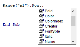
We will discuss a few of the most common properties below.
Change Font Color
There are a few ways to set font colors.
vbColor
The easiest way to set colors is with vbColors:
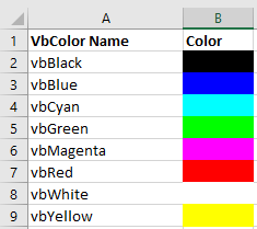
Range("a1").Font.Color = vbRedHowever, you’re very limited in terms of colors available. These are the only options available:
Color – RGB
You can also set colors based on RGB (Red Green Blue). Here you enter color values between 0-255 for Red, Green, and Blue. Using those three colors you can make any color:
Range("a1").Font.Color = RGB(255,255,0)ColorIndex
VBA / Excel also has a ColorIndex property. This makes pre-built colors available to you. However, they’re stored as Index numbers, which makes it hard to know what color is what:
Range("a1").Font.ColorIndex = …..We wrote an article about VBA Color codes, including a list of the VBA ColorIndex codes. There you can learn more about colors.
Font Size
This will set the font size to 12:
Range("a1").Font.Size = 12or to 16:
Range("a1").Font.Size = 16VBA Coding Made Easy
Stop searching for VBA code online. Learn more about AutoMacro — A VBA Code Builder that allows beginners to code procedures from scratch with minimal coding knowledge and with many time-saving features for all users!
Learn More
Bold Font
It is easy to set a cell font to Bold:
Range("A1").Font.Bold = Trueor to clear Bold formatting:
Range("A1").Font.Bold = FalseFont Name
To change a font name use the Name property:
Range("A1").Font.Name = "Calibri"Range("A1").Font.Name = "Arial"Range("A1").Font.Name = "Times New Roman"Cell Style
Excel offers the ability to create Cell “Styles”. Styles can be found in the Home Ribbon > Styles:
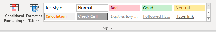
Styles allow you to save your desired Cell Formatting. Then assign that style to a new cell and all of the cell formatting is instantly applied. Including Font size, cell color, cell protections status, and anything else available from the Cell Formatting Menu:
Personally, for many of the models that I work on, I usually create an “Input” cell style:
Range("a1").Style = "Input"By using styles you can also easily identify cell types on your worksheet. The example below will loop through all the cells in the worksheet and change any cell with Style = “Input” to “InputLocked”:
Dim Cell as Range

For Each Cell in ActiveSheet.Cells
  If Cell.Style = "Input" then
    Cell.Style = "InputLocked"
  End If
Next CellВ VBA вы можете изменить свойства шрифта с помощью свойства шрифта VBA объекта Range. Введите следующий код в редактор VBA, и вы увидите список всех доступных вариантов:

Ниже мы обсудим несколько наиболее распространенных свойств.
Изменить цвет шрифта
Есть несколько способов установить цвета шрифта.
vbColor
Самый простой способ установить цвета — использовать vbColors:
| 1 | Диапазон («a1»). Font.Color = vbRed |
Однако количество доступных цветов очень ограничено. Это единственные доступные варианты:

Цвет — RGB
Вы также можете установить цвета на основе RGB (красный, зеленый, синий). Здесь вы вводите значения цвета от 0 до 255 для красного, зеленого и синего. Используя эти три цвета, вы можете сделать любой цвет:
| 1 | Диапазон («a1»). Font.Color = RGB (255,255,0) |
ColorIndex
VBA / Excel также имеет свойство ColorIndex. Это делает вам доступными предварительно созданные цвета. Однако они хранятся в виде порядковых номеров, что затрудняет определение того, что это за цвет:
| 1 | Диапазон («a1»). Font.ColorIndex =… |
Мы написали статью о цветовых кодах VBA, включая список кодов VBA ColorIndex. Там вы можете узнать больше о цветах.
Размер шрифта
Это установит размер шрифта на 12:
| 1 | Диапазон («a1»). Размер шрифта = 12 |
или до 16:
| 1 | Диапазон («a1»). Размер шрифта = 16 |
Жирный шрифт
Установить полужирный шрифт ячейки легко:
| 1 | Диапазон («A1»). Font.Bold = True |
или очистить форматирование полужирным шрифтом:
| 1 | Диапазон («A1»). Font.Bold = False |
Название шрифта
Чтобы изменить название шрифта, используйте Имя имущество:
| 1 | Диапазон («A1»). Font.Name = «Calibri» |
| 1 | Диапазон («A1»). Font.Name = «Arial» |
| 1 | Диапазон («A1»). Font.Name = «Times New Roman» |
Стиль ячейки
Excel предлагает возможность создавать «стили» ячеек. Стили можно найти в Главная Лента> Стили:

Стили позволяют сохранить желаемое форматирование ячеек. Затем назначьте этот стиль новой ячейке, и все форматирование ячейки будет немедленно применено. В том числе размер шрифта, цвет ячеек, состояние защиты ячеек и все остальное, что доступно в меню форматирования ячеек:

Лично для многих моделей, над которыми я работаю, я обычно создаю стиль ячейки «Вход»:
| 1 | Диапазон («a1»). Style = «Input» |
Используя стили, вы также можете легко определять типы ячеек на вашем листе. В приведенном ниже примере выполняется цикл по всем ячейкам на листе и изменяется любая ячейка со Style = «Input» на «InputLocked»:
| 1234567 | Тусклая ячейка как диапазонДля каждой ячейки в ActiveSheet.CellsЕсли Cell.Style = «Input», тогдаCell.Style = «InputLocked»Конец, еслиСледующая ячейка |
Вы поможете развитию сайта, поделившись страницей с друзьями
Change Font size
ActiveCell.Font.Size = 14
5 FREE EXCEL TEMPLATES
Plus Get 30% off any Purchase in the Simple Sheets Catalogue!
Embolden font
Selection.Font.Bold = True
Italicise font
Selection.Font.Italic = True
Underline font
Selection.Font.Underline = True
Font colour
5 FREE EXCEL TEMPLATES
Plus Get 30% off any Purchase in the Simple Sheets Catalogue!
Selection.Font.Color = vbRed
Also: vbBlack, vbBlue, vbCyan, vbGreen, vbMagenta, vbWhite,vbYellow
Selection.Font.Color = rgbBlueViolet
NB. Use CTRL SPACE to show the intellisense list of rgb colours
Selection.Font.Color = RGB(10, 201, 88)
ActiveCell.Font.ThemeColor = xlThemeColorAccent2
Selection.Font.ColorIndex = 49
This table shows the index number for colours in the default colour palette.

Background Colour of Cell/s
See font colour above for different ways of specifying colour.
Selection.Interior.Color = vbRed
Cell Borders
5 FREE EXCEL TEMPLATES
Plus Get 30% off any Purchase in the Simple Sheets Catalogue!
See font colour above for different ways of specifying colour.
Selection.Borders.Color = vbBlue
You can also specify properties such as weight and line style
With Selection.Borders
   .Color = vbBlue
   .Weight = xlMedium
   .LineStyle = xlDash
End With
Cell Alignment
Selection.HorizontalAlignment = xlCenter
Selection.VerticalAlignment = xlTop
To merge and center
Range("A1:E1").Merge
Range("A1").HorizontalAlignment = xlCenter
Number Format
ActiveCell.NumberFormat = "£#,##0.00;[Red]-£#,##0.00"
ActiveCell.NumberFormat = "0%"
ActiveCell.NumberFormat = "dd/mm/yyyy"
Use the custom format codes available in Excel’s Format | Cells dialog box.
By formatting cells and ranges you can give your worksheets a better look. Formatting applies to the following:
- The number format: Numeric, Date, Scientific …
- Text Alignment: Horizontal, Vertical, Orientation …
- Text Control: Wrap Text, Shrink to fit, Merge Cells …
- Text Direction
- Font Type: Calibri, Times new Roman …
- Font Style: Regular, Italic …
- Font Size: 8, 9, 10 …
- Font Color
- Font Effects: Strike through, Superscript …
- Borders: Style, Color, …
- Fill: Color, Pattern …
- Protection: Locked, Hidden
- …
As you can see there are a lot of different formatting options in excel. Listing all of them along with their syntax and examples would require an entire book. Fortunately excel has provided a tool for figuring out the syntax of the different formatting options, the macro recorder. Using the macro recorder you can figure out how to apply different formattings to ranges.
Jump To:
- Formatting Cells and the Macro Recorder
- Formatting Cell Borders
- Formatting Cell Protection
- Formatting Cell Font
- Formatting Cell Alignment
- Changing Cells Number Format
–
Formatting Cells and the Macro Recorder:
Below I will explain how to use macro recorder to figure out the required syntax for a specific type of formatting:
Step 1: In the developer tab click on Record Macro button:

Step 2: Click Ok:

Step 3: Apply the desired formatting to a range of cells. In this example I will change the color of the range to yellow and a apply a thick border to the exterior and interior sides of the range:


Step 4: Stop the macro recorder

Step 6: Open the visual basic editor. On the project window you will see a new folder which has been created called “Modules”. In this folder there will be a new file “Macro1”. By clicking on it you will see the generated Code:

For this example the code shown below has been generated:
Sub  Macro1()

'

' Macro1 Macro

'


'

    Range("I11:P16").Select

    Selection.Borders(xlDiagonalDown).LineStyle = xlNone

    Selection.Borders(xlDiagonalUp).LineStyle = xlNone

    With  Selection.Borders(xlEdgeLeft)

        .LineStyle = xlContinuous

        .ColorIndex = xlAutomatic

        .TintAndShade = 0

        .Weight = xlThick

    End With

    With  Selection.Borders(xlEdgeTop)

        .LineStyle = xlContinuous

        .ColorIndex = xlAutomatic

        .TintAndShade = 0

        .Weight = xlThick

    End With

    With  Selection.Borders(xlEdgeBottom)

        .LineStyle = xlContinuous

        .ColorIndex = xlAutomatic

        .TintAndShade = 0

        .Weight = xlThick

    End  With

    With  Selection.Borders(xlEdgeRight)

        .LineStyle = xlContinuous

        .ColorIndex = xlAutomatic

        .TintAndShade = 0

        .Weight = xlThick

    End With

    With  Selection.Borders(xlInsideVertical)

        .LineStyle = xlContinuous

        .ColorIndex = xlAutomatic

        .TintAndShade = 0

        .Weight = xlThick

    End  With

    With  Selection.Borders(xlInsideHorizontal)

        .LineStyle = xlContinuous

        .ColorIndex = xlAutomatic

        .TintAndShade = 0

        .Weight = xlThick

    End With

    With  Selection.Interior

        .Pattern = xlSolid

        .PatternColorIndex = xlAutomatic

        .Color = 65535

        .TintAndShade = 0

        .PatternTintAndShade = 0

    End  With

End  Sub
Remember that the macro recorder, records your every action. So if you have the macro recorder on and you start doing random things, the final generated code will become very long. So when you are trying to record a macro try to avoid any unnecessary actions. The first line of code you see is:
Range("I11:P16").Select
You will have to replace “I11:P16” with the range you are trying to modify . Also instead of using the select command you could directly use the range object:
Range("I11:P16").Borders(xlDiagonalDown).LineStyle = xlNone

Range("I11:P16").Borders(xlDiagonalUp).LineStyle = xlNone

With  Range("I11:P16").Borders(xlEdgeLeft)

    .LineStyle = xlContinuous

    .ColorIndex = xlAutomatic

    .TintAndShade = 0

    .Weight = xlThick

End With
I have brought some examples below.
–
Formatting Cell Borders:
The following example creates a border on the left edge of cell A1. The pattern is continuous and thick
With  Range("A1").Borders(xlEdgeLeft)

    .LineStyle = xlContinuous

    .ColorIndex = xlAutomatic

    .TintAndShade = 0

    .Weight = xlThick

End With
I have covered this topic in detail in the article below:
- Excel VBA, Borders
–
Formatting Cell Protection:
The following example locks and hides cells A1:
Range("A1").Locked = True

Range("A1").FormulaHidden = True
–
Formatting Cell Font:
The following code changes the font in cell A1 to arial, bold with size 9, applies strike through and single line underline formatting:
With  Range("A1").Font

    'font type

    .Name = "Arial"

    'font style

    .FontStyle = "Bold"

    'font size

    .Size = 9

    'uncheck strikethrough

    .Strikethrough = True

    'uncheck superscript

    .Superscript = False

    'uncheck subscript

    .Subscript = False

    .OutlineFont = False

    .Shadow = False

    'select single line underscript

    .Underline = xlUnderlineStyleSingle

    'set color to yellow

    .Color = 65535

    .TintAndShade = 0

    .ThemeFont = xlThemeFontNone

End With
For more information about formatting font properties please see the article below:
- VBA, Excel Font Formatting
–
Formatting Cell Alignment:
The following code sets the horizontal alignment of cell A1 to left, justifies its vertices alignment. Checks the wrap text and merge cell options and applies a -45 degree orientation:
With  Range("A1")

    'set the horizontal alignement to left

    .HorizontalAlignment = xlLeft

    'set the verticle alignment to justify

    .VerticalAlignment = xlJustify

    'check the wrap text option

    .WrapText = True

    'apply a -45 deg orientation

    .Orientation = -45

    'check the merge cell option

    .MergeCells = True

End With
For more information about cell alignment please see the article below:
- VBA Excel, Alignment
–
Changing Cells Number Format:
The following code changes cells A1’s number format to a date with the mm/dd/yy format:
Range("A1").NumberFormat = "mm/dd/yy;@"
See Also:
- VBA Excel, Font Formatting.
- VBA Excel, Alignment
- Excel VBA, Borders
If you need assistance with your code, or you are looking to hire a VBA programmer feel free to contact me. Also please visit my website www.software-solutions-online.com
Tagged with: Border, Cell Border, Cell Color, Cells, Color, Excel, Fill Color, Font, Font Color, Font Style, Formatting, Macro Recorder, Number Format, Ranges, Scientific, VBA
In this tutorial we’ll learn how to use Visual Basic for Applications (VBA) to modify text size and style in an Excel cell based on the cell content. This tutorial apply for Excel 365, 2021, 2019 and 2016.
Preliminaries
If you are new to Excel VBA development, I’ll recommend that before going through the tutorial you’ll look into our Excel VBA macro primer.
Before you start coding, you should enable your developer tab on Excel in the Ribbon, as otherwise you won’t be able to access your Visual Basic Editor.
Change your Excel cell text properties with VBA
Define your spreadsheet
We’ll start by defining an Excel spreadsheet that we will use as an example. Feel free to use it to follow along this tutorial.
- Open Microsoft Excel and create a new Macro Enabled Excel Workbook (.xlsm) named Excel_Macros.xlsm
- Save your Spreadsheet in your local drive.
- In the Sheet1 worksheet, go ahead and add the table below:

- Now, from the Ribbon, hit Formulas.
- Then hit Define Name.
- Define a Named Range on which you’ll apply your VBA code as shown below and hit OK.

Use Cell.Font VBA property to change font color and style
- Move to the Developer tab.
- Next go ahead and hit the Visual Basic button.
- In the left hand side Project Explorer, highlight the Excel_Macros.xlsm project then hit Insert and pick Module.
- A new VBA module named Module1 will be created.
- Go ahead and paste the following code in the newly created module:
Sub Color_Cell_Text_Condition()

Dim MyCell As Range
Dim StatValue As String
Dim StatusRange As Range

Set StatusRange = Range("Completion_Status")

'loop through all cells in the range
For Each MyCell In StatusRange

StatValue = MyCell.Value

'modify the cell text values as needed.
Select Case StatValue

    'green
    Case "Progressing"
    With MyCell.Font
        .Color = RGB(0, 255, 0)
        .Size = 14
        .Bold = True
     End With

    'orange
    Case "Pending Feedback"
    With MyCell.Font
        .Color = RGB(255, 141, 0)
        .Size = 14
        .Bold = True
    End With

    'red
    Case "Stuck"
    With MyCell.Font
        .Color = RGB(255, 0, 0)
        .Size = 14
        .Bold = True
    End With

End Select

Next MyCell

End Sub- Hit the Save button in your Visual Basic editor.
- Now hit Run and then pick Run Sub/UserForm (or simply hit F5).
- Move to your Sheet1 worksheet and notice the changes. Your table entries were assigned multiple color codes according to their text (using the RGB color function), and we also set the text to be bold and increase its size.

- If you haven’t saved your code, hit the Save button (or Ctrl+S), then also save your workbook.
Access your VBA Macro
- Note that your code is always available for you to run from the Macros command located in the View tab (or alternatively in Developer | Macros)
