
In this Article
- Ranges and Cells in VBA
- Cell Address
- Range of Cells
- Writing to Cells
- Reading from Cells
- Non Contiguous Cells
- Intersection of Cells
- Offset from a Cell or Range
- Setting Reference to a Range
- Resize a Range
- OFFSET vs Resize
- All Cells in Sheet
- UsedRange
- CurrentRegion
- Range Properties
- Last Cell in Sheet
- Last Used Row Number in a Column
- Last Used Column Number in a Row
- Cell Properties
- Copy and Paste
- AutoFit Contents
- More Range Examples
- For Each
- Sort
- Find
- Range Address
- Range to Array
- Array to Range
- Sum Range
- Count Range
Ranges and Cells in VBA
Excel spreadsheets store data in Cells. Cells are arranged into Rows and Columns. Each cell can be identified by the intersection point of it’s row and column (Exs. B3 or R3C2).
An Excel Range refers to one or more cells (ex. A3:B4)
Cell Address
A1 Notation
In A1 notation, a cell is referred to by it’s column letter (from A to XFD) followed by it’s row number(from 1 to 1,048,576). This is called a cell address.
In VBA you can refer to any cell using the Range Object.
' Refer to cell B4 on the currently active sheet
MsgBox Range("B4")

' Refer to cell B4 on the sheet named 'Data'
MsgBox Worksheets("Data").Range("B4")

' Refer to cell B4 on the sheet named 'Data' in another OPEN workbook
' named 'My Data'
MsgBox Workbooks("My Data").Worksheets("Data").Range("B4")
R1C1 Notation
In R1C1 Notation a cell is referred by R followed by Row Number then letter ‘C’ followed by the Column Number. eg B4 in R1C1 notation will be referred by R4C2. In VBA you use the Cells Object to use R1C1 notation:
' Refer to cell R[6]C[4] i.e D6
Cells(6, 4) = "D6"
Range of Cells
A1 Notation
To refer to a more than one cell use a “:” between the starting cell address and last cell address. The following will refer to all the cells from A1 to D10:
Range("A1:D10")
R1C1 Notation
To refer to a more than one cell use a “,” between the starting cell address and last cell address. The following will refer to all the cells from A1 to D10:
Range(Cells(1, 1), Cells(10, 4))Writing to Cells
To write values to a cell or contiguous group of cells, simple refer to the range, put an = sign and then write the value to be stored:
' Store F5 in cell with Address F6
Range("F6") = "F6"

' Store E6 in cell with Address R[6]C[5] i.e E6
Cells(6, 5) = "E6"

' Store A1:D10 in the range A1:D10
Range("A1:D10") = "A1:D10"
' or
Range(Cells(1, 1), Cells(10, 4)) = "A1:D10"
Reading from Cells
To read values from cells, simple refer to the variable to store the values, put an = sign and then refer to the range to be read:
Dim val1
Dim val2

' Read from cell F6
val1 = Range("F6")

' Read from cell E6
val2 = Cells(6, 5)

MsgBox val1
Msgbox val2
Note: To store values from a range of cells, you need to use an Array instead of a simple variable.
Non Contiguous Cells
To refer to non contiguous cells use a comma between the cell addresses:
' Store 10 in cells A1, A3, and A5
Range("A1,A3,A5") = 10


' Store 10 in cells A1:A3 and D1:D3)
Range("A1:A3, D1:D3") = 10
VBA Coding Made Easy
Stop searching for VBA code online. Learn more about AutoMacro — A VBA Code Builder that allows beginners to code procedures from scratch with minimal coding knowledge and with many time-saving features for all users!

Learn More
Intersection of Cells
To refer to non contiguous cells use a space between the cell addresses:
' Store 'Col D' in D1:D10
' which is Common between A1:D10 and D1:F10
Range("A1:D10 D1:G10") = "Col D"
Offset from a Cell or Range
Using the Offset function, you can move the reference from a given Range (cell or group of cells) by the specified number_of_rows, and number_of_columns.
Offset Syntax
Range.Offset(number_of_rows, number_of_columns)
Offset from a cell
' OFFSET from a cell A1
' Refer to cell itself
' Move 0 rows and 0 columns
Range("A1").Offset(0, 0) = "A1"

' Move 1 rows and 0 columns
Range("A1").Offset(1, 0) = "A2"

' Move 0 rows and 1 columns
Range("A1").Offset(0, 1) = "B1"

' Move 1 rows and 1 columns
Range("A1").Offset(1, 1) = "B2"

' Move 10 rows and 5 columns
Range("A1").Offset(10, 5) = "F11"
Offset from a Range
' Move Reference to Range A1:D4 by 4 rows and 4 columns
' New Reference is E5:H8
Range("A1:D4").Offset(4,4) = "E5:H8"
Setting Reference to a Range
To assign a range to a range variable: declare a variable of type Range then use the Set command to set it to a range. Please note that you must use the SET command as RANGE is an object:
' Declare a Range variable
Dim myRange as Range

' Set the variable to the range A1:D4
Set myRange = Range("A1:D4")

' Prints $A$1:$D$4
MsgBox myRange.Address
VBA Programming | Code Generator does work for you!
Resize a Range
Resize method of Range object changes the dimension of the reference range:
Dim myRange As Range

' Range to Resize
Set myRange = Range("A1:F4")

' Prints $A$1:$E$10
Debug.Print myRange.Resize(10, 5).Address
Top-left cell of the Resized range is same as the top-left cell of the original range
Resize Syntax
Range.Resize(number_of_rows, number_of_columns)
OFFSET vs Resize
Offset does not change the dimensions of the range but moves it by the specified number of rows and columns. Resize does not change the position of the original range but changes the dimensions to the specified number of rows and columns.
All Cells in Sheet
The Cells object refers to all the cells in the sheet (1048576 rows and 16384 columns).
' Clear All Cells in Worksheets
Cells.Clear
UsedRange
UsedRange property gives you the rectangular range from the top-left cell used cell to the right-bottom used cell of the active sheet.
Dim ws As Worksheet
Set ws = ActiveSheet

' $B$2:$L$14 if L2 is the first cell with any value
' and L14 is the last cell with any value on the
' active sheet
Debug.Print ws.UsedRange.Address
CurrentRegion
CurrentRegion property gives you the contiguous rectangular range from the top-left cell to the right-bottom used cell containing the referenced cell/range.
Dim myRange As Range

Set myRange = Range("D4:F6")

' Prints $B$2:$L$14
' If there is a filled path from D4:F16 to B2 AND L14
Debug.Print myRange.CurrentRegion.Address

' You can refer to a single starting cell also

Set myRange = Range("D4") ' Prints $B$2:$L$14
AutoMacro | Ultimate VBA Add-in | Click for Free Trial!
Range Properties
You can get Address, row/column number of a cell, and number of rows/columns in a range as given below:
Dim myRange As Range

Set myRange = Range("A1:F10")

' Prints $A$1:$F$10
Debug.Print myRange.Address

Set myRange = Range("F10")

' Prints 10 for Row 10
Debug.Print myRange.Row

' Prints 6 for Column F
Debug.Print myRange.Column

Set myRange = Range("E1:F5")
' Prints 5 for number of Rows in range
Debug.Print myRange.Rows.Count

' Prints 2 for number of Columns in range
Debug.Print myRange.Columns.Count
Last Cell in Sheet
You can use Rows.Count and Columns.Count properties with Cells object to get the last cell on the sheet:
' Print the last row number
' Prints 1048576
Debug.Print "Rows in the sheet: " & Rows.Count

' Print the last column number
' Prints 16384
Debug.Print "Columns in the sheet: " & Columns.Count

' Print the address of the last cell
' Prints $XFD$1048576
Debug.Print "Address of Last Cell in the sheet: " & Cells(Rows.Count, Columns.Count)
Last Used Row Number in a Column
END property takes you the last cell in the range, and End(xlUp) takes you up to the first used cell from that cell.
Dim lastRow As Long

lastRow = Cells(Rows.Count, "A").End(xlUp).Row
Last Used Column Number in a Row
Dim lastCol As Long

lastCol = Cells(1, Columns.Count).End(xlToLeft).Column
END property takes you the last cell in the range, and End(xlToLeft) takes you left to the first used cell from that cell.
You can also use xlDown and xlToRight properties to navigate to the first bottom or right used cells of the current cell.
AutoMacro | Ultimate VBA Add-in | Click for Free Trial!
Cell Properties
Common Properties
Here is code to display commonly used Cell Properties
Dim cell As Range
Set cell = Range("A1")

cell.Activate
Debug.Print cell.Address
' Print $A$1

Debug.Print cell.Value
' Prints 456
' Address

Debug.Print cell.Formula
' Prints =SUM(C2:C3)

' Comment
Debug.Print cell.Comment.Text

' Style
Debug.Print cell.Style

' Cell Format
Debug.Print cell.DisplayFormat.NumberFormat
Cell Font
Cell.Font object contains properties of the Cell Font:
Dim cell As Range

Set cell = Range("A1")

' Regular, Italic, Bold, and Bold Italic
cell.Font.FontStyle = "Bold Italic"
' Same as
cell.Font.Bold = True
cell.Font.Italic = True

' Set font to Courier
cell.Font.FontStyle = "Courier"

' Set Font Color
cell.Font.Color = vbBlue
' or
cell.Font.Color = RGB(255, 0, 0)

' Set Font Size
cell.Font.Size = 20
Copy and Paste
Paste All
Ranges/Cells can be copied and pasted from one location to another. The following code copies all the properties of source range to destination range (equivalent to CTRL-C and CTRL-V)
'Simple Copy
Range("A1:D20").Copy
Worksheets("Sheet2").Range("B10").Paste

'or
' Copy from Current Sheet to sheet named 'Sheet2'
Range("A1:D20").Copy destination:=Worksheets("Sheet2").Range("B10")
Paste Special
Selected properties of the source range can be copied to the destination by using PASTESPECIAL option:
' Paste the range as Values only
Range("A1:D20").Copy
Worksheets("Sheet2").Range("B10").PasteSpecial Paste:=xlPasteValues
Here are the possible options for the Paste option:
' Paste Special Types
xlPasteAll
xlPasteAllExceptBorders
xlPasteAllMergingConditionalFormats
xlPasteAllUsingSourceTheme
xlPasteColumnWidths
xlPasteComments
xlPasteFormats
xlPasteFormulas
xlPasteFormulasAndNumberFormats
xlPasteValidation
xlPasteValues
xlPasteValuesAndNumberFormats
AutoFit Contents
Size of rows and columns can be changed to fit the contents using AutoFit:
' Change size of rows 1 to 5 to fit contents
Rows("1:5").AutoFit

' Change size of Columns A to B to fit contents
Columns("A:B").AutoFit
More Range Examples
It is recommended that you use Macro Recorder while performing the required action through the GUI. It will help you understand the various options available and how to use them.
AutoMacro | Ultimate VBA Add-in | Click for Free Trial!
For Each
It is easy to loop through a range using For Each construct as show below:
For Each cell In Range("A1:B100")
    ' Do something with the cell
Next cell
At each iteration of the loop one cell in the range is assigned to the variable cell and statements in the For loop are executed for that cell. Loop exits when all the cells are processed.
Sort
Sort is a method of Range object. You can sort a range by specifying options for sorting to Range.Sort. The code below will sort the columns A:C based on key in cell C2. Sort Order can be xlAscending or xlDescending. Header:= xlYes should be used if first row is the header row.
   Columns("A:C").Sort key1:=Range("C2"), _
      order1:=xlAscending, Header:=xlYes
Find
Find is also a method of Range Object. It find the first cell having content matching the search criteria and returns the cell as a Range object. It return Nothing if there is no match.
Use FindNext method (or FindPrevious) to find next(previous) occurrence.
Following code will change the font to “Arial Black” for all cells in the range which start with “John”:
For Each c In Range("A1:A100")
    If c Like "John*" Then
        c.Font.Name = "Arial Black"
    End If
Next c
Following code will replace all occurrences of “To Test” to “Passed” in the range specified:
With Range("a1:a500")
    Set c = .Find("To Test", LookIn:=xlValues)
    If Not c Is Nothing Then
        firstaddress = c.Address
        Do
            c.Value = "Passed"
            Set c = .FindNext(c)
        Loop While Not c Is Nothing And c.Address <> firstaddress
    End If
End With
It is important to note that you must specify a range to use FindNext. Also you must provide a stopping condition otherwise the loop will execute forever. Normally address of the first cell which is found is stored in a variable and loop is stopped when you reach that cell again. You must also check for the case when nothing is found to stop the loop.
Range Address
Use Range.Address to get the address in A1 Style
MsgBox Range("A1:D10").Address
' or
Debug.Print Range("A1:D10").Address
Use xlReferenceStyle (default is xlA1) to get addres in R1C1 style
MsgBox Range("A1:D10").Address(ReferenceStyle:=xlR1C1)
' or
Debug.Print Range("A1:D10").Address(ReferenceStyle:=xlR1C1)
This is useful when you deal with ranges stored in variables and want to process for certain addresses only.
AutoMacro | Ultimate VBA Add-in | Click for Free Trial!
Range to Array
It is faster and easier to transfer a range to an array and then process the values. You should declare the array as Variant to avoid calculating the size required to populate the range in the array. Array’s dimensions are set to match number of values in the range.
Dim DirArray As Variant
' Store the values in the range to the Array

DirArray = Range("a1:a5").Value

' Loop to process the values
For Each c In DirArray
    Debug.Print c
Next
Array to Range
After processing you can write the Array back to a Range. To write the Array in the example above to a Range you must specify a Range whose size matches the number of elements in the Array.
Use the code below to write the Array to the range D1:D5:
Range("D1:D5").Value = DirArray

Range("D1:H1").Value = Application.Transpose(DirArray)
Please note that you must Transpose the Array if you write it to a row.
Sum Range
SumOfRange = Application.WorksheetFunction.Sum(Range("A1:A10"))
Debug.Print SumOfRange
You can use many functions available in Excel in your VBA code by specifying Application.WorkSheetFunction. before the Function Name as in the example above.
Count Range
' Count Number of Cells with Numbers in the Range
CountOfCells = Application.WorksheetFunction.Count(Range("A1:A10"))
Debug.Print CountOfCells

' Count Number of Non Blank Cells in the Range
CountOfNonBlankCells = Application.WorksheetFunction.CountA(Range("A1:A10"))
Debug.Print CountOfNonBlankCells
Written by: Vinamra Chandra
“It is a capital mistake to theorize before one has data”- Sir Arthur Conan Doyle
This post covers everything you need to know about using Cells and Ranges in VBA. You can read it from start to finish as it is laid out in a logical order. If you prefer you can use the table of contents below to go to a section of your choice.
Topics covered include Offset property, reading values between cells, reading values to arrays and formatting cells.
A Quick Guide to Ranges and Cells
| Function | Takes | Returns | Example | Gives |
|---|---|---|---|---|
|
Range |
cell address | multiple cells | .Range(«A1:A4») | $A$1:$A$4 |
| Cells | row, column | one cell | .Cells(1,5) | $E$1 |
| Offset | row, column | multiple cells | Range(«A1:A2») .Offset(1,2) |
$C$2:$C$3 |
| Rows | row(s) | one or more rows | .Rows(4) .Rows(«2:4») |
$4:$4 $2:$4 |
| Columns | column(s) | one or more columns | .Columns(4) .Columns(«B:D») |
$D:$D $B:$D |
Download the Code
The Webinar
If you are a member of the VBA Vault, then click on the image below to access the webinar and the associated source code.
(Note: Website members have access to the full webinar archive.)

Introduction
This is the third post dealing with the three main elements of VBA. These three elements are the Workbooks, Worksheets and Ranges/Cells. Cells are by far the most important part of Excel. Almost everything you do in Excel starts and ends with Cells.
Generally speaking, you do three main things with Cells
- Read from a cell.
- Write to a cell.
- Change the format of a cell.
Excel has a number of methods for accessing cells such as Range, Cells and Offset.These can cause confusion as they do similar things and can lead to confusion
In this post I will tackle each one, explain why you need it and when you should use it.
Let’s start with the simplest method of accessing cells – using the Range property of the worksheet.
Important Notes
I have recently updated this article so that is uses Value2.
You may be wondering what is the difference between Value, Value2 and the default:
' Value2
Range("A1").Value2 = 56

' Value
Range("A1").Value = 56

' Default uses value
Range("A1") = 56
Using Value may truncate number if the cell is formatted as currency. If you don’t use any property then the default is Value.
It is better to use Value2 as it will always return the actual cell value(see this article from Charle Williams.)
The Range Property
The worksheet has a Range property which you can use to access cells in VBA. The Range property takes the same argument that most Excel Worksheet functions take e.g. “A1”, “A3:C6” etc.
The following example shows you how to place a value in a cell using the Range property.
' https://excelmacromastery.com/
Public Sub WriteToCell()

    ' Write number to cell A1 in sheet1 of this workbook
    ThisWorkbook.Worksheets("Sheet1").Range("A1").Value2 = 67

    ' Write text to cell A2 in sheet1 of this workbook
    ThisWorkbook.Worksheets("Sheet1").Range("A2").Value2 = "John Smith"

    ' Write date to cell A3 in sheet1 of this workbook
    ThisWorkbook.Worksheets("Sheet1").Range("A3").Value2 = #11/21/2017#

End Sub
As you can see Range is a member of the worksheet which in turn is a member of the Workbook. This follows the same hierarchy as in Excel so should be easy to understand. To do something with Range you must first specify the workbook and worksheet it belongs to.
For the rest of this post I will use the code name to reference the worksheet.

The following code shows the above example using the code name of the worksheet i.e. Sheet1 instead of ThisWorkbook.Worksheets(“Sheet1”).
' https://excelmacromastery.com/
Public Sub UsingCodeName()

    ' Write number to cell A1 in sheet1 of this workbook
    Sheet1.Range("A1").Value2 = 67

    ' Write text to cell A2 in sheet1 of this workbook
    Sheet1.Range("A2").Value2 = "John Smith"

    ' Write date to cell A3 in sheet1 of this workbook
    Sheet1.Range("A3").Value2 = #11/21/2017#

End Sub
You can also write to multiple cells using the Range property
' https://excelmacromastery.com/
Public Sub WriteToMulti()

    ' Write number to a range of cells
    Sheet1.Range("A1:A10").Value2 = 67

    ' Write text to multiple ranges of cells
    Sheet1.Range("B2:B5,B7:B9").Value2 = "John Smith"

End Sub
You can download working examples of all the code from this post from the top of this article.
The Cells Property of the Worksheet
The worksheet object has another property called Cells which is very similar to range. There are two differences
- Cells returns a range of one cell only.
- Cells takes row and column as arguments.
The example below shows you how to write values to cells using both the Range and Cells property
' https://excelmacromastery.com/
Public Sub UsingCells()

    ' Write to A1
    Sheet1.Range("A1").Value2 = 10
    Sheet1.Cells(1, 1).Value2  = 10

    ' Write to A10
    Sheet1.Range("A10").Value2 = 10
    Sheet1.Cells(10, 1).Value2  = 10

    ' Write to E1
    Sheet1.Range("E1").Value2 = 10
    Sheet1.Cells(1, 5).Value2  = 10

End Sub
You may be wondering when you should use Cells and when you should use Range. Using Range is useful for accessing the same cells each time the Macro runs.
For example, if you were using a Macro to calculate a total and write it to cell A10 every time then Range would be suitable for this task.
Using the Cells property is useful if you are accessing a cell based on a number that may vary. It is easier to explain this with an example.
In the following code, we ask the user to specify the column number. Using Cells gives us the flexibility to use a variable number for the column.
' https://excelmacromastery.com/
Public Sub WriteToColumn()

    Dim UserCol As Integer

    ' Get the column number from the user
    UserCol = Application.InputBox(" Please enter the column...", Type:=1)

    ' Write text to user selected column
    Sheet1.Cells(1, UserCol).Value2 = "John Smith"

End Sub
In the above example, we are using a number for the column rather than a letter.
To use Range here would require us to convert these values to the letter/number cell reference e.g. “C1”. Using the Cells property allows us to provide a row and a column number to access a cell.
Sometimes you may want to return more than one cell using row and column numbers. The next section shows you how to do this.
Using Cells and Range together
As you have seen you can only access one cell using the Cells property. If you want to return a range of cells then you can use Cells with Ranges as follows
' https://excelmacromastery.com/
Public Sub UsingCellsWithRange()

    With Sheet1
        ' Write 5 to Range A1:A10 using Cells property
        .Range(.Cells(1, 1), .Cells(10, 1)).Value2 = 5

        ' Format Range B1:Z1 to be bold
        .Range(.Cells(1, 2), .Cells(1, 26)).Font.Bold = True

    End With

End Sub
As you can see, you provide the start and end cell of the Range. Sometimes it can be tricky to see which range you are dealing with when the value are all numbers. Range has a property called Address which displays the letter/ number cell reference of any range. This can come in very handy when you are debugging or writing code for the first time.
In the following example we print out the address of the ranges we are using:
' https://excelmacromastery.com/
Public Sub ShowRangeAddress()

    ' Note: Using underscore allows you to split up lines of code
    With Sheet1

        ' Write 5 to Range A1:A10 using Cells property
        .Range(.Cells(1, 1), .Cells(10, 1)).Value2 = 5
        Debug.Print "First address is : " _
            + .Range(.Cells(1, 1), .Cells(10, 1)).Address

        ' Format Range B1:Z1 to be bold
        .Range(.Cells(1, 2), .Cells(1, 26)).Font.Bold = True
        Debug.Print "Second address is : " _
            + .Range(.Cells(1, 2), .Cells(1, 26)).Address

    End With

End Sub
In the example I used Debug.Print to print to the Immediate Window. To view this window select View->Immediate Window(or Ctrl G)


You can download all the code for this post from the top of this article.
The Offset Property of Range
Range has a property called Offset. The term Offset refers to a count from the original position. It is used a lot in certain areas of programming. With the Offset property you can get a Range of cells the same size and a certain distance from the current range. The reason this is useful is that sometimes you may want to select a Range based on a certain condition. For example in the screenshot below there is a column for each day of the week. Given the day number(i.e. Monday=1, Tuesday=2 etc.) we need to write the value to the correct column.

We will first attempt to do this without using Offset.
' https://excelmacromastery.com/
' This sub tests with different values
Public Sub TestSelect()

    ' Monday
    SetValueSelect 1, 111.21
    ' Wednesday
    SetValueSelect 3, 456.99
    ' Friday
    SetValueSelect 5, 432.25
    ' Sunday
    SetValueSelect 7, 710.17

End Sub

' Writes the value to a column based on the day
Public Sub SetValueSelect(lDay As Long, lValue As Currency)

    Select Case lDay
        Case 1: Sheet1.Range("H3").Value2 = lValue
        Case 2: Sheet1.Range("I3").Value2 = lValue
        Case 3: Sheet1.Range("J3").Value2 = lValue
        Case 4: Sheet1.Range("K3").Value2 = lValue
        Case 5: Sheet1.Range("L3").Value2 = lValue
        Case 6: Sheet1.Range("M3").Value2 = lValue
        Case 7: Sheet1.Range("N3").Value2 = lValue
    End Select

End Sub
As you can see in the example, we need to add a line for each possible option. This is not an ideal situation. Using the Offset Property provides a much cleaner solution
' https://excelmacromastery.com/
' This sub tests with different values
Public Sub TestOffset()

    DayOffSet 1, 111.01
    DayOffSet 3, 456.99
    DayOffSet 5, 432.25
    DayOffSet 7, 710.17

End Sub

Public Sub DayOffSet(lDay As Long, lValue As Currency)

    ' We use the day value with offset specify the correct column
    Sheet1.Range("G3").Offset(, lDay).Value2 = lValue

End Sub
As you can see this solution is much better. If the number of days in increased then we do not need to add any more code. For Offset to be useful there needs to be some kind of relationship between the positions of the cells. If the Day columns in the above example were random then we could not use Offset. We would have to use the first solution.
One thing to keep in mind is that Offset retains the size of the range. So .Range(“A1:A3”).Offset(1,1) returns the range B2:B4. Below are some more examples of using Offset
' https://excelmacromastery.com/
Public Sub UsingOffset()

    ' Write to B2 - no offset
    Sheet1.Range("B2").Offset().Value2 = "Cell B2"

    ' Write to C2 - 1 column to the right
    Sheet1.Range("B2").Offset(, 1).Value2 = "Cell C2"

    ' Write to B3 - 1 row down
    Sheet1.Range("B2").Offset(1).Value2 = "Cell B3"

    ' Write to C3 - 1 column right and 1 row down
    Sheet1.Range("B2").Offset(1, 1).Value2 = "Cell C3"

    ' Write to A1 - 1 column left and 1 row up
    Sheet1.Range("B2").Offset(-1, -1).Value2 = "Cell A1"

    ' Write to range E3:G13 - 1 column right and 1 row down
    Sheet1.Range("D2:F12").Offset(1, 1).Value2 = "Cells E3:G13"

End Sub
Using the Range CurrentRegion
CurrentRegion returns a range of all the adjacent cells to the given range.
In the screenshot below you can see the two current regions. I have added borders to make the current regions clear.

A row or column of blank cells signifies the end of a current region.
You can manually check the CurrentRegion in Excel by selecting a range and pressing Ctrl + Shift + *.
If we take any range of cells within the border and apply CurrentRegion, we will get back the range of cells in the entire area.
For example
Range(“B3”).CurrentRegion will return the range B3:D14
Range(“D14”).CurrentRegion will return the range B3:D14
Range(“C8:C9”).CurrentRegion will return the range B3:D14
and so on
How to Use
We get the CurrentRegion as follows
' Current region will return B3:D14 from above example
Dim rg As Range
Set rg = Sheet1.Range("B3").CurrentRegion
Read Data Rows Only
Read through the range from the second row i.e.skipping the header row
' Current region will return B3:D14 from above example
Dim rg As Range
Set rg = Sheet1.Range("B3").CurrentRegion

' Start at row 2 - row after header
Dim i As Long
For i = 2 To rg.Rows.Count
    ' current row, column 1 of range
    Debug.Print rg.Cells(i, 1).Value2
Next i
Remove Header
Remove header row(i.e. first row) from the range. For example if range is A1:D4 this will return A2:D4
' Current region will return B3:D14 from above example
Dim rg As Range
Set rg = Sheet1.Range("B3").CurrentRegion

' Remove Header
Set rg = rg.Resize(rg.Rows.Count - 1).Offset(1)

' Start at row 1 as no header row
Dim i As Long
For i = 1 To rg.Rows.Count
    ' current row, column 1 of range
    Debug.Print rg.Cells(i, 1).Value2
Next i
Using Rows and Columns as Ranges
If you want to do something with an entire Row or Column you can use the Rows or Columns property of the Worksheet. They both take one parameter which is the row or column number you wish to access
' https://excelmacromastery.com/
Public Sub UseRowAndColumns()

    ' Set the font size of column B to 9
    Sheet1.Columns(2).Font.Size = 9

    ' Set the width of columns D to F
    Sheet1.Columns("D:F").ColumnWidth = 4

    ' Set the font size of row 5 to 18
    Sheet1.Rows(5).Font.Size = 18

End Sub
Using Range in place of Worksheet
You can also use Cells, Rows and Columns as part of a Range rather than part of a Worksheet. You may have a specific need to do this but otherwise I would avoid the practice. It makes the code more complex. Simple code is your friend. It reduces the possibility of errors.
The code below will set the second column of the range to bold. As the range has only two rows the entire column is considered B1:B2
' https://excelmacromastery.com/
Public Sub UseColumnsInRange()

    ' This will set B1 and B2 to be bold
    Sheet1.Range("A1:C2").Columns(2).Font.Bold = True

End Sub
You can download all the code for this post from the top of this article.
Reading Values from one Cell to another
In most of the examples so far we have written values to a cell. We do this by placing the range on the left of the equals sign and the value to place in the cell on the right. To write data from one cell to another we do the same. The destination range goes on the left and the source range goes on the right.
The following example shows you how to do this:
' https://excelmacromastery.com/
Public Sub ReadValues()

    ' Place value from B1 in A1
    Sheet1.Range("A1").Value2 = Sheet1.Range("B1").Value2

    ' Place value from B3 in sheet2 to cell A1
    Sheet1.Range("A1").Value2 = Sheet2.Range("B3").Value2

    ' Place value from B1 in cells A1 to A5
    Sheet1.Range("A1:A5").Value2 = Sheet1.Range("B1").Value2

    ' You need to use the "Value" property to read multiple cells
    Sheet1.Range("A1:A5").Value2 = Sheet1.Range("B1:B5").Value2

End Sub
As you can see from this example it is not possible to read from multiple cells. If you want to do this you can use the Copy function of Range with the Destination parameter
' https://excelmacromastery.com/
Public Sub CopyValues()

    ' Store the copy range in a variable
    Dim rgCopy As Range
    Set rgCopy = Sheet1.Range("B1:B5")

    ' Use this to copy from more than one cell
    rgCopy.Copy Destination:=Sheet1.Range("A1:A5")

    ' You can paste to multiple destinations
    rgCopy.Copy Destination:=Sheet1.Range("A1:A5,C2:C6")

End Sub
The Copy function copies everything including the format of the cells. It is the same result as manually copying and pasting a selection. You can see more about it in the Copying and Pasting Cells section.
Using the Range.Resize Method
When copying from one range to another using assignment(i.e. the equals sign), the destination range must be the same size as the source range.
Using the Resize function allows us to resize a range to a given number of rows and columns.
For example:
' https://excelmacromastery.com/
Sub ResizeExamples()

    ' Prints A1
    Debug.Print Sheet1.Range("A1").Address

    ' Prints A1:A2
    Debug.Print Sheet1.Range("A1").Resize(2, 1).Address

    ' Prints A1:A5
    Debug.Print Sheet1.Range("A1").Resize(5, 1).Address

    ' Prints A1:D1
    Debug.Print Sheet1.Range("A1").Resize(1, 4).Address

    ' Prints A1:C3
    Debug.Print Sheet1.Range("A1").Resize(3, 3).Address

End Sub
When we want to resize our destination range we can simply use the source range size.
In other words, we use the row and column count of the source range as the parameters for resizing:
' https://excelmacromastery.com/
Sub Resize()

    Dim rgSrc As Range, rgDest As Range

    ' Get all the data in the current region
    Set rgSrc = Sheet1.Range("A1").CurrentRegion

      ' Get the range destination
    Set rgDest = Sheet2.Range("A1")
    Set rgDest = rgDest.Resize(rgSrc.Rows.Count, rgSrc.Columns.Count)

    rgDest.Value2 = rgSrc.Value2

End Sub
We can do the resize in one line if we prefer:
' https://excelmacromastery.com/
Sub ResizeOneLine()

    Dim rgSrc As Range

    ' Get all the data in the current region
    Set rgSrc = Sheet1.Range("A1").CurrentRegion

    With rgSrc
        Sheet2.Range("A1").Resize(.Rows.Count, .Columns.Count).Value2 = .Value2
    End With

End Sub
Reading Values to variables
We looked at how to read from one cell to another. You can also read from a cell to a variable. A variable is used to store values while a Macro is running. You normally do this when you want to manipulate the data before writing it somewhere. The following is a simple example using a variable. As you can see the value of the item to the right of the equals is written to the item to the left of the equals.
' https://excelmacromastery.com/
Public Sub UseVariables()

    ' Create
    Dim number As Long

    ' Read number from cell
    number = Sheet1.Range("A1").Value2

    ' Add 1 to value
    number = number + 1

    ' Write new value to cell
    Sheet1.Range("A2").Value2 = number

End Sub
To read text to a variable you use a variable of type String:
' https://excelmacromastery.com/
Public Sub UseVariableText()

    ' Declare a variable of type string
    Dim text As String

    ' Read value from cell
    text = Sheet1.Range("A1").Value2

    ' Write value to cell
    Sheet1.Range("A2").Value2 = text

End Sub
You can write a variable to a range of cells. You just specify the range on the left and the value will be written to all cells in the range.
' https://excelmacromastery.com/
Public Sub VarToMulti()

    ' Read value from cell
    Sheet1.Range("A1:B10").Value2 = 66

End Sub
You cannot read from multiple cells to a variable. However you can read to an array which is a collection of variables. We will look at doing this in the next section.
How to Copy and Paste Cells
If you want to copy and paste a range of cells then you do not need to select them. This is a common error made by new VBA users.
Note: We normally use Range.Copy when we want to copy formats, formulas, validation. If we want to copy values it is not the most efficient method.
I have written a complete guide to copying data in Excel VBA here.
You can simply copy a range of cells like this:
Range("A1:B4").Copy Destination:=Range("C5")
Using this method copies everything – values, formats, formulas and so on. If you want to copy individual items you can use the PasteSpecial property of range.
It works like this
Range("A1:B4").Copy
Range("F3").PasteSpecial Paste:=xlPasteValues
Range("F3").PasteSpecial Paste:=xlPasteFormats
Range("F3").PasteSpecial Paste:=xlPasteFormulas
The following table shows a full list of all the paste types
| Paste Type |
|---|
| xlPasteAll |
| xlPasteAllExceptBorders |
| xlPasteAllMergingConditionalFormats |
| xlPasteAllUsingSourceTheme |
| xlPasteColumnWidths |
| xlPasteComments |
| xlPasteFormats |
| xlPasteFormulas |
| xlPasteFormulasAndNumberFormats |
| xlPasteValidation |
| xlPasteValues |
| xlPasteValuesAndNumberFormats |
Reading a Range of Cells to an Array
You can also copy values by assigning the value of one range to another.
Range("A3:Z3").Value2 = Range("A1:Z1").Value2
The value of range in this example is considered to be a variant array. What this means is that you can easily read from a range of cells to an array. You can also write from an array to a range of cells. If you are not familiar with arrays you can check them out in this post.
The following code shows an example of using an array with a range:
' https://excelmacromastery.com/
Public Sub ReadToArray()

    ' Create dynamic array
    Dim StudentMarks() As Variant

    ' Read 26 values into array from the first row
    StudentMarks = Range("A1:Z1").Value2

    ' Do something with array here

    ' Write the 26 values to the third row
    Range("A3:Z3").Value2 = StudentMarks

End Sub
Keep in mind that the array created by the read is a 2 dimensional array. This is because a spreadsheet stores values in two dimensions i.e. rows and columns
Going through all the cells in a Range
Sometimes you may want to go through each cell one at a time to check value.
You can do this using a For Each loop shown in the following code
' https://excelmacromastery.com/
Public Sub TraversingCells()

    ' Go through each cells in the range
    Dim rg As Range
    For Each rg In Sheet1.Range("A1:A10,A20")
        ' Print address of cells that are negative
        If rg.Value < 0 Then
            Debug.Print rg.Address + " is negative."
        End If
    Next

End Sub
You can also go through consecutive Cells using the Cells property and a standard For loop.
The standard loop is more flexible about the order you use but it is slower than a For Each loop.
' https://excelmacromastery.com/
Public Sub TraverseCells()

    ' Go through cells from A1 to A10
    Dim i As Long
    For i = 1 To 10
        ' Print address of cells that are negative
        If Range("A" & i).Value < 0 Then
            Debug.Print Range("A" & i).Address + " is negative."
        End If
    Next

    ' Go through cells in reverse i.e. from A10 to A1
    For i = 10 To 1 Step -1
        ' Print address of cells that are negative
        If Range("A" & i) < 0 Then
            Debug.Print Range("A" & i).Address + " is negative."
        End If
    Next

End Sub
Formatting Cells
Sometimes you will need to format the cells the in spreadsheet. This is actually very straightforward. The following example shows you various formatting you can add to any range of cells
' https://excelmacromastery.com/
Public Sub FormattingCells()

    With Sheet1

        ' Format the font
        .Range("A1").Font.Bold = True
        .Range("A1").Font.Underline = True
        .Range("A1").Font.Color = rgbNavy

        ' Set the number format to 2 decimal places
        .Range("B2").NumberFormat = "0.00"
        ' Set the number format to a date
        .Range("C2").NumberFormat = "dd/mm/yyyy"
        ' Set the number format to general
        .Range("C3").NumberFormat = "General"
        ' Set the number format to text
        .Range("C4").NumberFormat = "Text"

        ' Set the fill color of the cell
        .Range("B3").Interior.Color = rgbSandyBrown

        ' Format the borders
        .Range("B4").Borders.LineStyle = xlDash
        .Range("B4").Borders.Color = rgbBlueViolet

    End With

End Sub
Main Points
The following is a summary of the main points
- Range returns a range of cells
- Cells returns one cells only
- You can read from one cell to another
- You can read from a range of cells to another range of cells.
- You can read values from cells to variables and vice versa.
- You can read values from ranges to arrays and vice versa
- You can use a For Each or For loop to run through every cell in a range.
- The properties Rows and Columns allow you to access a range of cells of these types
What’s Next?
Free VBA Tutorial If you are new to VBA or you want to sharpen your existing VBA skills then why not try out the The Ultimate VBA Tutorial.
Related Training: Get full access to the Excel VBA training webinars and all the tutorials.
(NOTE: Planning to build or manage a VBA Application? Learn how to build 10 Excel VBA applications from scratch.)
When working with Excel, most of your time is spent in the worksheet area – dealing with cells and ranges.
And if you want to automate your work in Excel using VBA, you need to know how to work with cells and ranges using VBA.
There are a lot of different things you can do with ranges in VBA (such as select, copy, move, edit, etc.).
So to cover this topic, I will break this tutorial into sections and show you how to work with cells and ranges in Excel VBA using examples.
Let’s get started.
All the codes I mention in this tutorial need to be placed in the VB Editor. Go to the ‘Where to Put the VBA Code‘ section to know how it works.
If you’re interested in learning VBA the easy way, check out my Online Excel VBA Training.
Selecting a Cell / Range in Excel using VBA
To work with cells and ranges in Excel using VBA, you don’t need to select it.
In most of the cases, you are better off not selecting cells or ranges (as we will see).
Despite that, it’s important you go through this section and understand how it works. This will be crucial in your VBA learning and a lot of concepts covered here will be used throughout this tutorial.
So let’s start with a very simple example.
Selecting a Single Cell Using VBA
If you want to select a single cell in the active sheet (say A1), then you can use the below code:
Sub SelectCell()
Range("A1").Select
End Sub
The above code has the mandatory ‘Sub’ and ‘End Sub’ part, and a line of code that selects cell A1.
Range(“A1”) tells VBA the address of the cell that we want to refer to.
Select is a method of the Range object and selects the cells/range specified in the Range object. The cell references need to be enclosed in double quotes.
This code would show an error in case a chart sheet is an active sheet. A chart sheet contains charts and is not widely used. Since it doesn’t have cells/ranges in it, the above code can’t select it and would end up showing an error.
Note that since you want to select the cell in the active sheet, you just need to specify the cell address.
But if you want to select the cell in another sheet (let’s say Sheet2), you need to first activate Sheet2 and then select the cell in it.
Sub SelectCell()
Worksheets("Sheet2").Activate
Range("A1").Select
End Sub
Similarly, you can also activate a workbook, then activate a specific worksheet in it, and then select a cell.
Sub SelectCell()
Workbooks("Book2.xlsx").Worksheets("Sheet2").Activate
Range("A1").Select
End Sub
Note that when you refer to workbooks, you need to use the full name along with the file extension (.xlsx in the above code). In case the workbook has never been saved, you don’t need to use the file extension.
Now, these examples are not very useful, but you will see later in this tutorial how we can use the same concepts to copy and paste cells in Excel (using VBA).
Just as we select a cell, we can also select a range.
In case of a range, it could be a fixed size range or a variable size range.
In a fixed size range, you would know how big the range is and you can use the exact size in your VBA code. But with a variable-sized range, you have no idea how big the range is and you need to use a little bit of VBA magic.
Let’s see how to do this.
Selecting a Fix Sized Range
Here is the code that will select the range A1:D20.
Sub SelectRange()
Range("A1:D20").Select
End Sub
Another way of doing this is using the below code:
Sub SelectRange()
Range("A1", "D20").Select
End Sub
The above code takes the top-left cell address (A1) and the bottom-right cell address (D20) and selects the entire range. This technique becomes useful when you’re working with variably sized ranges (as we will see when the End property is covered later in this tutorial).
If you want the selection to happen in a different workbook or a different worksheet, then you need to tell VBA the exact names of these objects.
For example, the below code would select the range A1:D20 in Sheet2 worksheet in the Book2 workbook.
Sub SelectRange()
Workbooks("Book2.xlsx").Worksheets("Sheet1").Activate
Range("A1:D20").Select
End Sub
Now, what if you don’t know how many rows are there. What if you want to select all the cells that have a value in it.
In these cases, you need to use the methods shown in the next section (on selecting variably sized range).
Selecting a Variably Sized Range
There are different ways you can select a range of cells. The method you choose would depend on how the data is structured.
In this section, I will cover some useful techniques that are really useful when you work with ranges in VBA.
Select Using CurrentRange Property
In cases where you don’t know how many rows/columns have the data, you can use the CurrentRange property of the Range object.
The CurrentRange property covers all the contiguous filled cells in a data range.
Below is the code that will select the current region that holds cell A1.
Sub SelectCurrentRegion()
Range("A1").CurrentRegion.Select
End Sub
The above method is good when you have all data as a table without any blank rows/columns in it.
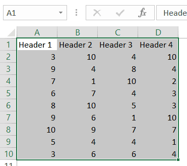
But in case you have blank rows/columns in your data, it will not select the ones after the blank rows/columns. In the image below, the CurrentRegion code selects data till row 10 as row 11 is blank.
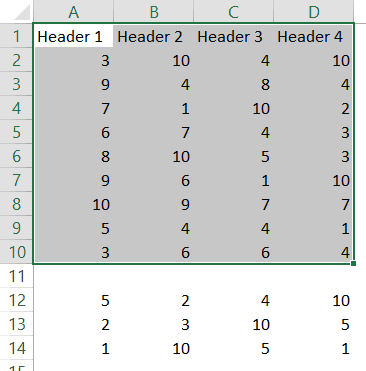
In such cases, you may want to use the UsedRange property of the Worksheet Object.
Select Using UsedRange Property
UsedRange allows you to refer to any cells that have been changed.
So the below code would select all the used cells in the active sheet.
Sub SelectUsedRegion()
ActiveSheet.UsedRange.Select
End Sub
Note that in case you have a far-off cell that has been used, it would be considered by the above code and all the cells till that used cell would be selected.
Select Using the End Property
Now, this part is really useful.
The End property allows you to select the last filled cell. This allows you to mimic the effect of Control Down/Up arrow key or Control Right/Left keys.
Let’s try and understand this using an example.
Suppose you have a dataset as shown below and you want to quickly select the last filled cells in column A.
The problem here is that data can change and you don’t know how many cells are filled. If you have to do this using keyboard, you can select cell A1, and then use Control + Down arrow key, and it will select the last filled cell in the column.
Now let’s see how to do this using VBA. This technique comes in handy when you want to quickly jump to the last filled cell in a variably-sized column
Sub GoToLastFilledCell()
Range("A1").End(xlDown).Select
End Sub
The above code would jump to the last filled cell in column A.
Similarly, you can use the End(xlToRight) to jump to the last filled cell in a row.
Sub GoToLastFilledCell()
Range("A1").End(xlToRight).Select
End Sub
Now, what if you want to select the entire column instead of jumping to the last filled cell.
You can do that using the code below:
Sub SelectFilledCells()
Range("A1", Range("A1").End(xlDown)).Select
End Sub
In the above code, we have used the first and the last reference of the cell that we need to select. No matter how many filled cells are there, the above code will select all.
Remember the example above where we selected the range A1:D20 by using the following line of code:
Range(“A1″,”D20”)
Here A1 was the top-left cell and D20 was the bottom-right cell in the range. We can use the same logic in selecting variably sized ranges. But since we don’t know the exact address of the bottom-right cell, we used the End property to get it.
In Range(“A1”, Range(“A1”).End(xlDown)), “A1” refers to the first cell and Range(“A1”).End(xlDown) refers to the last cell. Since we have provided both the references, the Select method selects all the cells between these two references.
Similarly, you can also select an entire data set that has multiple rows and columns.
The below code would select all the filled rows/columns starting from cell A1.
Sub SelectFilledCells()
Range("A1", Range("A1").End(xlDown).End(xlToRight)).Select
End Sub
In the above code, we have used Range(“A1”).End(xlDown).End(xlToRight) to get the reference of the bottom-right filled cell of the dataset.
Difference between Using CurrentRegion and End
If you’re wondering why use the End property to select the filled range when we have the CurrentRegion property, let me tell you the difference.
With End property, you can specify the start cell. For example, if you have your data in A1:D20, but the first row are headers, you can use the End property to select the data without the headers (using the code below).
Sub SelectFilledCells()
Range("A2", Range("A2").End(xlDown).End(xlToRight)).Select
End Sub
But the CurrentRegion would automatically select the entire dataset, including the headers.
So far in this tutorial, we have seen how to refer to a range of cells using different ways.
Now let’s see some ways where we can actually use these techniques to get some work done.
Copy Cells / Ranges Using VBA
As I mentioned at the beginning of this tutorial, selecting a cell is not necessary to perform actions on it. You will see in this section how to copy cells and ranges without even selecting these.
Let’s start with a simple example.
Copying Single Cell
If you want to copy cell A1 and paste it into cell D1, the below code would do it.
Sub CopyCell()
Range("A1").Copy Range("D1")
End Sub
Note that the copy method of the range object copies the cell (just like Control +C) and pastes it in the specified destination.
In the above example code, the destination is specified in the same line where you use the Copy method. If you want to make your code even more readable, you can use the below code:
Sub CopyCell()
Range("A1").Copy Destination:=Range("D1")
End Sub
The above codes will copy and paste the value as well as formatting/formulas in it.
As you might have already noticed, the above code copies the cell without selecting it. No matter where you’re on the worksheet, the code will copy cell A1 and paste it on D1.
Also, note that the above code would overwrite any existing code in cell D2. If you want Excel to let you know if there is already something in cell D1 without overwriting it, you can use the code below.
Sub CopyCell()
If Range("D1") <> "" Then
Response = MsgBox("Do you want to overwrite the existing data", vbYesNo)
End If
If Response = vbYes Then
Range("A1").Copy Range("D1")
End If
End Sub
Copying a Fix Sized Range
If you want to copy A1:D20 in J1:M20, you can use the below code:
Sub CopyRange()
Range("A1:D20").Copy Range("J1")
End Sub
In the destination cell, you just need to specify the address of the top-left cell. The code would automatically copy the exact copied range into the destination.
You can use the same construct to copy data from one sheet to the other.
The below code would copy A1:D20 from the active sheet to Sheet2.
Sub CopyRange()
Range("A1:D20").Copy Worksheets("Sheet2").Range("A1")
End Sub
The above copies the data from the active sheet. So make sure the sheet that has the data is the active sheet before running the code. To be safe, you can also specify the worksheet’s name while copying the data.
Sub CopyRange()
Worksheets("Sheet1").Range("A1:D20").Copy Worksheets("Sheet2").Range("A1")
End Sub
The good thing about the above code is that no matter which sheet is active, it will always copy the data from Sheet1 and paste it in Sheet2.
You can also copy a named range by using its name instead of the reference.
For example, if you have a named range called ‘SalesData’, you can use the below code to copy this data to Sheet2.
Sub CopyRange()
Range("SalesData").Copy Worksheets("Sheet2").Range("A1")
End Sub
If the scope of the named range is the entire workbook, you don’t need to be on the sheet that has the named range to run this code. Since the named range is scoped for the workbook, you can access it from any sheet using this code.
If you have a table with the name Table1, you can use the below code to copy it to Sheet2.
Sub CopyTable()
Range("Table1[#All]").Copy Worksheets("Sheet2").Range("A1")
End Sub
You can also copy a range to another Workbook.
In the following example, I copy the Excel table (Table1), into the Book2 workbook.
Sub CopyCurrentRegion()
Range("Table1[#All]").Copy Workbooks("Book2.xlsx").Worksheets("Sheet1").Range("A1")
End Sub
This code would work only if the Workbook is already open.
Copying a Variable Sized Range
One way to copy variable sized ranges is to convert these into named ranges or Excel Table and the use the codes as shown in the previous section.
But if you can’t do that, you can use the CurrentRegion or the End property of the range object.
The below code would copy the current region in the active sheet and paste it in Sheet2.
Sub CopyCurrentRegion()
Range("A1").CurrentRegion.Copy Worksheets("Sheet2").Range("A1")
End Sub
If you want to copy the first column of your data set till the last filled cell and paste it in Sheet2, you can use the below code:
Sub CopyCurrentRegion()
Range("A1", Range("A1").End(xlDown)).Copy Worksheets("Sheet2").Range("A1")
End Sub
If you want to copy the rows as well as columns, you can use the below code:
Sub CopyCurrentRegion()
Range("A1", Range("A1").End(xlDown).End(xlToRight)).Copy Worksheets("Sheet2").Range("A1")
End Sub
Note that all these codes don’t select the cells while getting executed. In general, you will find only a handful of cases where you actually need to select a cell/range before working on it.
Assigning Ranges to Object Variables
So far, we have been using the full address of the cells (such as Workbooks(“Book2.xlsx”).Worksheets(“Sheet1”).Range(“A1”)).
To make your code more manageable, you can assign these ranges to object variables and then use those variables.
For example, in the below code, I have assigned the source and destination range to object variables and then used these variables to copy data from one range to the other.
Sub CopyRange()
Dim SourceRange As Range
Dim DestinationRange As Range
Set SourceRange = Worksheets("Sheet1").Range("A1:D20")
Set DestinationRange = Worksheets("Sheet2").Range("A1")
SourceRange.Copy DestinationRange
End Sub
We start by declaring the variables as Range objects. Then we assign the range to these variables using the Set statement. Once the range has been assigned to the variable, you can simply use the variable.
Enter Data in the Next Empty Cell (Using Input Box)
You can use the Input boxes to allow the user to enter the data.
For example, suppose you have the data set below and you want to enter the sales record, you can use the input box in VBA. Using a code, we can make sure that it fills the data in the next blank row.
Sub EnterData()
Dim RefRange As Range
Set RefRange = Range("A1").End(xlDown).Offset(1, 0)
Set ProductCategory = RefRange.Offset(0, 1)
Set Quantity = RefRange.Offset(0, 2)
Set Amount = RefRange.Offset(0, 3)
RefRange.Value = RefRange.Offset(-1, 0).Value + 1
ProductCategory.Value = InputBox("Product Category")
Quantity.Value = InputBox("Quantity")
Amount.Value = InputBox("Amount")
End Sub
The above code uses the VBA Input box to get the inputs from the user, and then enters the inputs into the specified cells.
Note that we didn’t use exact cell references. Instead, we have used the End and Offset property to find the last empty cell and fill the data in it.
This code is far from usable. For example, if you enter a text string when the input box asks for quantity or amount, you will notice that Excel allows it. You can use an If condition to check whether the value is numeric or not and then allow it accordingly.
Looping Through Cells / Ranges
So far we can have seen how to select, copy, and enter the data in cells and ranges.
In this section, we will see how to loop through a set of cells/rows/columns in a range. This could be useful when you want to analyze each cell and perform some action based on it.
For example, if you want to highlight every third row in the selection, then you need to loop through and check for the row number. Similarly, if you want to highlight all the negative cells by changing the font color to red, you need to loop through and analyze each cell’s value.
Here is the code that will loop through the rows in the selected cells and highlight alternate rows.
Sub HighlightAlternateRows()
Dim Myrange As Range
Dim Myrow As Range
Set Myrange = Selection
For Each Myrow In Myrange.Rows
If Myrow.Row Mod 2 = 0 Then
Myrow.Interior.Color = vbCyan
End If
Next Myrow
End Sub
The above code uses the MOD function to check the row number in the selection. If the row number is even, it gets highlighted in cyan color.
Here is another example where the code goes through each cell and highlights the cells that have a negative value in it.
Sub HighlightAlternateRows()
Dim Myrange As Range
Dim Mycell As Range
Set Myrange = Selection
For Each Mycell In Myrange
If Mycell < 0 Then
Mycell.Interior.Color = vbRed
End If
Next Mycell
End Sub
Note that you can do the same thing using Conditional Formatting (which is dynamic and a better way to do this). This example is only for the purpose of showing you how looping works with cells and ranges in VBA.
Where to Put the VBA Code
Wondering where the VBA code goes in your Excel workbook?
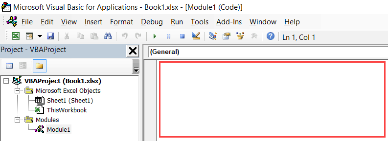
Excel has a VBA backend called the VBA editor. You need to copy and paste the code in the VB Editor module code window.
Here are the steps to do this:
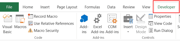
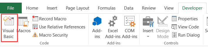
- Go to the Developer tab.

- Click on the Visual Basic option. This will open the VB editor in the backend.
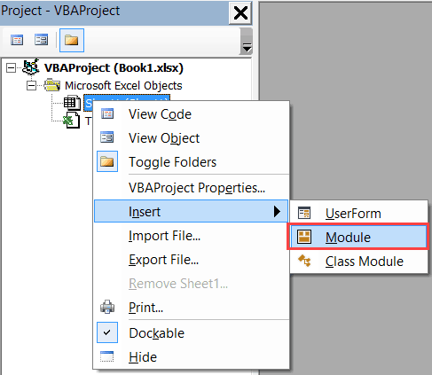
- In the Project Explorer pane in the VB Editor, right-click on any object for the workbook in which you want to insert the code. If you don’t see the Project Explorer, go to the View tab and click on Project Explorer.
- Go to Insert and click on Module. This will insert a module object for your workbook.

- Copy and paste the code in the module window.

You May Also Like the Following Excel Tutorials:
- Working with Worksheets using VBA.
- Working with Workbooks using VBA.
- Creating User-Defined Functions in Excel.
- For Next Loop in Excel VBA – A Beginner’s Guide with Examples.
- How to Use Excel VBA InStr Function (with practical EXAMPLES).
- Excel VBA Msgbox.
- How to Record a Macro in Excel.
- How to Run a Macro in Excel.
- How to Create an Add-in in Excel.
- Excel Personal Macro Workbook | Save & Use Macros in All Workbooks.
- Excel VBA Events – An Easy (and Complete) Guide.
- Excel VBA Error Handling.
- How to Sort Data in Excel using VBA (A Step-by-Step Guide).
- 24 Useful Excel Macro Examples for VBA Beginners (Ready-to-use).
Cells are actually cells of the worksheet and in VBA when we refer to cells as a range property we are actually referring to the exact cells, in other words, cell is used with range property and the method of using cells property is as follows Range(.Cells(1,1)) now cells (1,1) means the cell A1 the first argument is for the row and second is for the column reference.
VBA Cell References
You don’t need any special introduction about what is a VBA cell. In VBA concepts, cells are also the same, no different from normal excel cells. Follow this article to have more knowledge of the VBA cells concept.
Table of contents
- VBA Cell References
- What is VBA Range & VBA Cell?
- The Formula of CELLS Property in VBA
- #1 – How to Use CELLS Property in VBA?
- #2 – How to Use CELLS Property with Range Object?
- #3 – Cells Property with Loops
- Things to Remember in VBA Cells
- Recommended Articles
What is VBA Range & VBA Cell?
I am sure this is the question running in your mind right now. In VBA, Range is an object, but Cell is a property in an excel sheet. In VBA, we have two ways of referencing a cell object one through Range, and another one is through Cells.
For example, if you want to reference cell C5, you can use two methods to refer to the cell C5.
Using Range Method: Range (“C5”)
Using Cells Method: Cells (5, 3)
Similarly, if you want to insert value “Hi” to C5 cell, then you can use the below code.
Using Range Method: Range (“C5”).Value = “Hi”
Using Cells Method: Cells (5, 3).Value = “Hi”
Now, if you want to select multiple cells, we can only select through the Range object. For example, if I want to select cells from A1 to A10, below is the code.
Code: Range (“A1: A10”).Select
But unfortunately, we can only reference one cellCell reference in excel is referring the other cells to a cell to use its values or properties. For instance, if we have data in cell A2 and want to use that in cell A1, use =A2 in cell A1, and this will copy the A2 value in A1.read more at a time by using CELLS property. We can use Cells with a Range object like the below.
Range (“A1: C10”).Cells(5,2) mean in the range A1 to C10 fifth row and second column i.e., B5 cell.
The Formula of CELLS Property in VBA
Take a look at the formula of CELLS property.

- Row Index: This nothing but which row we are referencing.
- Column Index: This nothing but which column we are referencing.
- Cells (1, 1) means A1 cell, Cells (2, 1) means A2 cell, Cells (1, 2) means B1 cell.
- Cells (2, 2) means B2 cell, Cells (10, 3) means C10 cell, Cells (15, 5) means E15 cell.
#1 – How to Use CELLS Property in VBA?
Now I will teach you how to use these CELLS property in VBA.
You can download this VBA Cells Excel Template here – VBA Cells Excel Template
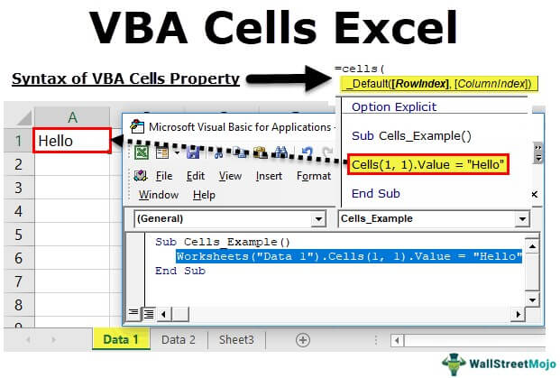
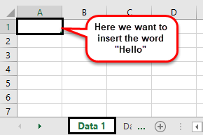
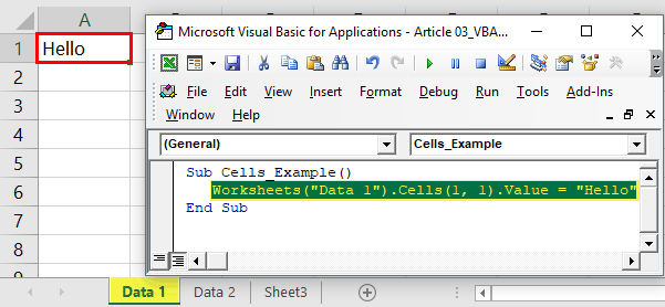
Assume you are working in the sheet name called Data 1, and you want to insert a value “Hello” to the cell A1.
The Below code would do that for you.
Sub Cells_Example()
Cells(1, 1).Value = "Hello"
End Sub
Result:
Now I will go to the sheet name called Data 2 and will run the code. Even there, it will insert the word “Hello.”
Actually, we can combine the CELLS property with a particular sheet name as well. To refer a particular sheet, use the WORKSHEET object.
Worksheets(“Data 1”).Cells(1,1).Value = “Hello”
This will insert the word “Hello” to the sheet “Data 1” irrespective of which sheet you are in.
#2 – How to Use CELLS Property with Range Object?
Actually, we can use CELLS property with a RANGE object. For example, look at the below code.
Range("C2:E8").Cells(1, 1).Select

For better understanding, I have entered a few numbers in the excel sheet.
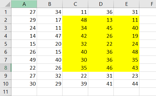
The above code Range(“C2:E8”).Cells(1, 1).Select says in the range C2 to E8 select the first cell. Run this code and see what happens.
Sub Cells_Example()
Range("C2:E8").Cells(1, 1).Select
End Sub

It has selected the cell C2. But Cells (1, 1) means A1 cell, isn’t it?
The reason it has selected the cell C2 because using range object, we have insisted on the range as C2 to E8, so Cells property treats the range from C2 to E8, not from regular A1 cell. In this example, C2 is the first row and first column, so Cells (1, 1).select means C2 cell.
Now I will change the code to Range(“C2: E8”).Cells(3, 2).Select and see what happens.
Run this code and check which cell actually it will select.
Sub Cells_Example()
Range("C2:E8").Cells(3, 2).Select
End Sub
It has selected the cell D4 i.e., No 26. Cells (3,2) mean starting from C2 cell moved down by 3 rows and move 2 columns to the right i.e., D4 cell.
#3 – Cells Property with Loops
CELLS property with loops has a very good relationship in VBA. Let’s look at the example of inserting serial numbers from 1 to 10 using FOR LOOP. Copy and paste the below code to your module.
Sub Cells_Example()
Dim i As Integer
   For i = 1 To 10
     Cells(i, 1).Value = i
     Next i
End Sub
Here I have declared the variable I as an integer.
Then I have applied FOR LOOP with I = 1 to 10 i.e., and the loop needs to run 10 times.
Cells(i,1).value = i
This means that when the loop first runs, the value of “I” will be 1, so wherever the value of “I” is 1 i.e., Cell(1,1).value = 1
When the loop returns the value of “I” for the second time, it is 2, so wherever the value of “I” is, it is 2. i.e., Cell(2,1).value = 2
This loop will run for 10 times and insert I value from A1 to A10.
Things to Remember in VBA Cells
- CELLS is property, but the RANGE is an Object. We can use property with objects but not object to the property.
- When the range is supplied, cells will consider only that range, not the regular range.
- Cells (1, 2) is B1 cell, similarly Cells (1, ”B”) is also B1 cell.
Recommended Articles
This has been a Guide to VBA Cells. Here we learn how to use VBA Cell Reference Property with Range Object along with practical examples and downloadable excel templates. Below you can find some useful excel VBA articles –
- Select Cell in VBAVBA select cell assists the users to pick any particular cell using various methods like Macro recorder, range object, select statement, CELLS property and cell reference.read more
- Use VBA Range Function
- VLookup in Excel VBAThe functionality of VLOOKUP in VBA is similar to that of VLOOKUP in a worksheet, and the method of using VLOOKUP in VBA is through an application. Method WorksheetFunctionread more
- Excel VBA Range CellsThe range property of VBA is used to refer to any data, cells, or selection. It is an inbuilt property that allows us to access any part of the worksheet. Using the range property for a single cell-like range is referred to as range cells.read more
# Ways to refer to a single cell
The simplest way to refer to a single cell on the current Excel worksheet is simply to enclose the A1 form of its reference in square brackets:
Note that square brackets are just convenient syntactic sugar (opens new window) for the Evaluate method of the Application object, so technically, this is identical to the following code:
You could also call the Cells method which takes a row and a column and returns a cell reference.
Remember that whenever you pass a row and a column to Excel from VBA, the row is always first, followed by the column, which is confusing because it is the opposite of the common A1 notation where the column appears first.
In both of these examples, we did not specify a worksheet, so Excel will use the active sheet (the sheet that is in front in the user interface). You can specify the active sheet explicitly:
Or you can provide the name of a particular sheet:
There are a wide variety of methods that can be used to get from one range to another. For example, the Rows method can be used to get to the individual rows of any range, and the Cells method can be used to get to individual cells of a row or column, so the following code refers to cell C1:
# Creating a Range
A Range (opens new window) cannot be created or populated the same way a string would:
It is considered best practice to qualify your references (opens new window), so from now on we will use the same approach here.
More about Creating Object Variables (e.g. Range) on MSDN (opens new window) . More about Set Statement on MSDN (opens new window).
There are different ways to create the same Range:
Note in the example that Cells(2, 1) is equivalent to Range(«A2»). This is because Cells returns a Range object.
Some sources: Chip Pearson-Cells Within Ranges (opens new window); MSDN-Range Object (opens new window); John Walkenback-Referring To Ranges In Your VBA Code (opens new window).
Also note that in any instance where a number is used in the declaration of the range, and the number itself is outside of quotation marks, such as Range(«A» & 2), you can swap that number for a variable that contains an integer/long. For example:
If you are using double loops, Cells is better:
# Offset Property
- Offset(Rows, Columns) — The operator used to statically reference another point from the current cell. Often used in loops. It should be understood that positive numbers in the rows section moves right, wheres as negatives move left. With the columns section positives move down and negatives move up.
i.e
This code selects B2, puts a new string there, then moves that string back to A1 afterwards clearing out B2.
# Saving a reference to a cell in a variable
To save a reference to a cell in a variable, you must use the Set syntax, for example:
later…
Why is the Set keyword required? Set tells Visual Basic that the value on the right hand side of the = is meant to be an object.
# How to Transpose Ranges (Horizontal to Vertical & vice versa)
Note: Copy/PasteSpecial also has a Paste Transpose option which updates the transposed cells’ formulas as well.
# Syntax
- Set — The operator used to set a reference to an object, such as a Range
- For Each — The operator used to loop through every item in a collection
Note that the variable names r, cell and others can be named however you like but should be named appropriately so the code is easier to understand for you and others.
Свойство Cells объекта Range в VBA Excel, представляющее коллекцию ячеек заданного диапазона. Обращение к ячейкам диапазона с помощью свойства Cells.
Range.Cells – свойство, возвращающее коллекцию всех ячеек указанного диапазона.
Свойство Cells объекта Worksheet
Обращение к ячейке «A1» активного рабочего листа с помощью свойства Cells:
|
‘по индексу (порядковому номеру) ячейки MsgBox Cells(1).Address ‘Результат: $A$1 ‘по номеру строки и номеру столбца MsgBox Cells(1, 1).Address ‘Результат: $A$1 ‘по номеру строки и буквенному обозначению столбца MsgBox Cells(1, «A»).Address ‘Результат: $A$1 |
В данном случае в качестве объекта Range выступает диапазон всего активного рабочего листа (ActiveSheet). Полный путь к ячейке «A1» можно записать так:
|
MsgBox ThisWorkbook.ActiveSheet.Cells(1).Address ‘Результат: $A$1 MsgBox ThisWorkbook.ActiveSheet.Cells(1, 1).Address ‘Результат: $A$1 MsgBox ThisWorkbook.ActiveSheet.Cells(1, «A»).Address ‘Результат: $A$1 |
Обращение в VBA Excel к ячейке «C5» с помощью свойства Cells по имени рабочего листа (Worksheet) в другой книге Excel:
|
MsgBox Workbooks(«Книга1.xlsm»).Worksheets(«Лист1»).Cells(65539).Address ‘Результат: $C$5 в Excel 2016 MsgBox Workbooks(«Книга1.xlsm»).Worksheets(«Лист1»).Cells(5, 3).Address ‘Результат: $C$5 MsgBox Workbooks(«Книга1.xlsm»).Worksheets(«Лист1»).Cells(5, «C»).Address ‘Результат: $C$5 |
Обращение к диапазону «C5:G10» с помощью свойства Cells активного рабочего листа:
|
MsgBox Range(Cells(5, 3), Cells(10, 7)).Address ‘Результат: $C$5:$G$10 |
Обращение в VBA Excel к ячейкам заданного диапазона с помощью свойства Cells рассмотрим на коллекции ячеек диапазона «C5:G10». Обращаться будем к ячейке «D8» активного листа:
|
MsgBox Range(«C5:G10»).Cells(17).Address ‘Результат: $D$8 MsgBox Range(«C5:G10»).Cells(4, 2).Address ‘Результат: $D$8 MsgBox Range(«C5:G10»).Cells(4, «B»).Address ‘Результат: $D$8 |
Обратите внимание, что отсчет номеров строк, номеров и буквенных обозначений столбцов для указания адреса ячейки внутри диапазона ведется от верхней левой ячейки данного диапазона.
Обход диапазона ячеек циклом
Обход ячеек циклом For Each… Next
Обход ячеек циклом For Each… Next — это самый простой способ обхода всех ячеек заданного диапазона. Он может быть применен, например, для присвоения ячейкам свойств и значений или поиска ячейки с определенным свойством или значением.
Присвоение ячейкам диапазона «B3:F10» числовых значений, соответствующих их порядковым номерам (индексам) в диапазоне:
|
Sub Primer1() Dim myCell As Range, n As Long For Each myCell In Range(«B3:F10») n = n + 1 myCell = n Next End Sub |
Поиск в диапазоне «B3:F10», заполненном предыдущим кодом VBA Excel значениями, ячейки со значением «27», окрашивание ее в зеленый цвет и выход из цикла:
|
Sub Primer2() Dim myCell As Range, n As Long For Each myCell In Range(«B3:F10») If myCell = 27 Then myCell.Interior.Color = vbGreen Exit For End If Next End Sub |
Обход диапазона циклом For… Next
Цикл For… Next позволяет указывать переменные в качестве индексов ячеек или номеров строк и столбцов для обхода ячеек заданного диапазона.
Присвоение ячейкам диапазона «B3:F10» числовых значений, соответствующих их порядковым номерам (индексам) в диапазоне, с помощью цикла For… Next:
|
Sub Primer3() Dim i As Long, n As Long With Range(«B3:F10») n = .Cells.Count For i = 1 To n .Cells(i) = i Next End With End Sub |
Если в блоке с оператором With вместо строки .Cells(i) = i указать строку без точки впереди — Cells(i) = i, то свойство Cells будет относиться не к диапазону Range("B3:F10"), а к рабочему листу (объекту ActiveSheet). В этом случае, порядковыми номерами будут заполнены первые 40 ячеек первой строки активного рабочего листа.
Применение в качестве параметров свойства Cells объекта Range переменных, задающих номера строк и номера столбцов указанного диапазона при обходе его ячеек циклом For… Next:
|
Sub Primer4() Dim i1 As Long, i2 As Long, r As Long, c As Long With Range(«B3:F10») r = .Rows.Count c = .Columns.Count For i1 = 1 To r For i2 = 1 To c .Cells(i1, i2) = (i1 — 1) * c + i2 Next Next End With End Sub |
Номер ячейки на рабочем листе
Определение порядкового номера (индекса) активной ячейки на рабочем листе Excel с помощью кода VBA:
|
Sub Primer5() Dim n As Double n = (ActiveCell.Row — 1) * CDbl(Cells.Columns.Count) + ActiveCell.Column MsgBox n End Sub |
Introduction to Range and Cells in VBA
When you look around in an Excel workbook, you will find that everything works around cells. A cell and a range of cells are where you store your data, and then everything starts.
To make the best of VBA, you need to learn how to use cells and ranges in your codes. For this, you need to have a solid understanding of Range objects. By using it, you can refer to cells in your codes in the following ways:
- A single cell.
- A range of cells
- A row or a column
- A three-dimensional range
The RANGE OBJECT is a part of Excel’s Object Hierarchy: Application ➜ Workbooks ➜ Worksheets ➜ Range and besides inside the worksheet. So if you are writing code to refer to the RANGE object it would be like this:
Application.Workbook(“Workbook-Name”).Worksheets(“Sheet-Name”).RangeBy referring to a cell or range of cells, you can do the following things:
- You can read the value from it.
- You can enter a value in it.
- And, you can make changes to the format.
To do all these things, you need to learn to refer to a cell or a range of cells, and in the next section of this tutorial, you will learn to refer to a cell using different ways.
To refer to a cell or a range of cells, you can use three different ways.
- Range Property
- Cells Property
- Offset Property
Well, which one is best out of these depends on your requirement, but it is worth learning all three so that you can choose which one is perfect for you.
So let’s get started.
Range Property
Range property is the most common and popular way to refer to a range in your VBA codes. With Range property, you simply need to refer to the cell address. Let me tell you the syntax.
expression.range(address)Here the expression is a variable representing a VBA object. So if you need to refer to the cell A1, the line of code you need to write would be:
Application.Workbook(“Book1”).Worksheets(“Sheet1”).Range(“A1”)The above code tells VBA that you are referring to cell A1 which is in the worksheet “Sheet1” and workbook ”Book1”.
Note: Whenever you type a cell address in the range object, make sure to wrap it in double quotation marks. But here’s one thing to understand. As you are using VBA in Excel there’s no need to use the word “Application”. So the code would be:
Workbook(“Book1”).Worksheets(“Sheet1”).Range(“A1”)And if you are in the Book1 there you can further trim down your code:
Worksheets(“Sheet1”).Range(“A1”)But, if you are already in the worksheet “Sheet1” then you can further trim down your code and can only use:
Range(“A1”)Now, let’s say if you want to refer to a full range of cells (i.e., multiple cells) you need to write the code in the following way:
Range("A1:A5")In the above code, you have referred to the range A1 to A5 which consists of the five cells. You can also refer to a named range using the range object. Let’s say you have named range with the name of “Sales Discount” to refer to this you can write a code like this:
Range("Sales Discount")If you want to refer to a non-continues range then you need to do something like this:
Range("A1:B5,D5:G10")And if you want to refer to an entire row or a column then you need to enter code like the below:
Range("1:1")
Range("A:A")
At this point, you have a clear understanding of how to refer to a cell and the range of cells. But to make it best with this you need to learn how to use this to do other things.
here we have a complete list of tutorials that you can use to learn to work with ranges and cells in VBA
- How to SET (Get and Change) Cell Value using a VBA Code
- How to Select a Range using VBA in Excel
- How to Create a Named Range using VBA (Static + Dynamic) in Excel
- How to Merge and Unmerge Cells in Excel using a VBA Code
- How to Check IF a Cell is Empty using VBA in Excel
- VBA ClearContents (from a Cell, Range, or Entire Worksheet)
- Excel VBA Font (Color, Size, Type, and Bold)
- How to AutoFit (Rows, Column, or the Entire Worksheet) using VBA
- How to use OFFSET Property with the Range Object or a Cell in VBA
- VBA Wrap Text (Cell, Range, and Entire Worksheet)
- How to Copy a CellRange to Another Sheet using VBA
- How to use Range/Cell as a Variable in VBA in Excel
- How to Find Last Rows, Column, and Cell using VBA in Excel
- How to use ActiveCell in VBA in Excel
- How to Refer to the UsedRange using VBA in Excel
- How to Change Row Height/Column Width using VBA in Excel
- How to SELECT ALL the Cells in a Worksheet using a VBA Code
- How to Insert a Row using VBA in Excel
- How to Insert a Column using VBA in Excel
1. Select and Activate a Cell
If you want to select a cell then you can use the Range. Select method. Let’s say if you want to select cell A5 then all you need to do is specify the range and then add “.Select” after that.
Range(“A1”).SelectThis code tells VBA to select cell A5 and if you want to select a range of cells then you just need to refer to that range and simply add “.Select” after that.
Range(“A1:A5”).SelectThere’s also another method that you can use to activate a cell.
Range(“A1”).ActivateHere you need to remember that you can activate only one cell at a time. Even if you specify a range with the “.Activate” method, it will select that range but the active cell will be the first cell of the range.
2. Enter a Value in a Cell
By using the range property you can enter a value in a cell or a range of cells. Let’s understand how it works using a simple example:
Range("A1").Value = "ExcelChamps"In the above example, you have specified the A1 as a range and after that, you have added “.Value” which tells VBA to access the value property of the cell.
The next thing you have is the equals sign and then the value which you want to enter (you need to use double quotation marks if you are entering a text value). For a number, the code would like this:
Range("A1").Value = 9988And if you want to enter a value into a range of cells, I mean multiple cells, then all you need to do is specify that range.
Range("A1:A5").Value = "ExcelChamps"And, here’s the code if you are referring to the non-continues range.
Range("A1:A5 , E2:E3").Value = "ExcelChamps"3. Copy and Paste a Cell/Range
With Range property, you can use the “.Copy” method to copy and cell and then paste it into a destination cell. Let’s say if you need to copy the cell A5 the code for this would be:
Range("A5").Copy When you run this code it will simply copy cell A5 but the next thing is to paste this copied cell to a destination cell. For this, you need to add the keyword destination after it and followed by the cell where you want to paste it. So if you want to copy cell A1 and then want to paste it to the cell E5, the code would be:
Range("A1").Copy Destination:=Range("E5")In the same way, if you are dealing with a range of multiple cells then the code would be like:
Range("A1:A5").Copy Destination:=Range("E5:E9")If you have copied a range of cells and then if you have mentioned one cell as the destination range, VBA will copy the entire copied range the starting from the cell you have specified as a destination.
Range("A1:A5").Copy Destination:=Range("B1")When you run the above code, VBA will copy range A1:A5 and will paste it to the B1:B5 even though you have mentioned only B1 as the destination range.
Tip: Just like the “.Copy” method you can use the “.Cut” method to cut a cell and then simply use a destination to paste it.
4. Use Font Property with Range Property
With the range property, you can access the font property of a cell which helps you to change all the font settings. There are a total of 18 different properties for the font which you can access. Let’s say if you want to make the text BOLD in cell A1, the code would be:
Range("A1").Font.Bold = TrueThis code tells VBA to access the BOLD property of the font which is inside the range A1 and you have set this property to TRUE. Now, let’s say you want to apply strikethrough to cell A1, this time the code would be:
As I said there are a total of 18 different properties you can use, so make sure to check out all of these to see which one is useful for you.
5. Clear Formatting from a Cell
By using the “.ClearFormats” method you can remove only the format from a cell or a range of cells. All you need to do is add “.ClearFormat” after specifying the range, like below:
Range("A1").ClearFormatsWhen you run the code above it clears all the formatting from cell A1 and if you want to do it for an entire range, you know what to do, Right?
Range("A1:A5").ClearFormatsNow the above code will simply remove the formatting from the range A1 to A5.
Cells Property
Apart from the RANGE property, you can use the “Cells” property to refer to a cell or a range of cells in your worksheet. In cell property, instead of using the cell reference, you need to enter the column number and row number of the cell.
expression.Cells(Row_Number, Column_Number)Here the expression is a VBA object and Row_Number is the row number of the cell and Column_Number is the column of the cell. So if you want to refer to the cell A5 you can use the code below code:
Cells(5,1)Now, this code tells VBA to refer to the cell which is at row number five and at column number one. As its syntax says you need to enter column number as address but the reality is you can also use the column alphabet if you want just by wrapping it in double quotation marks.
The below code will also refer to the cell A5:
Cells(5,"A")And to VBA to select it simply add “.Select” at the end.
Cells(5,1).SelectThe above code will select cell A5 which is in the 5th row and in the first column of the worksheet.
OFFSET Property
If you want to play well with ranges in VBA you need to know how to use the OFFSET property. It helps to refer to a cell that is a particular number of rows and columns away from another cell.
Let’s say your active cell is B5 right now and you want to navigate to the cell which is 3 columns right and 1 row down from B5, you can do this OFFSET. Below is the syntax which you need to use for the OFFSET:
expression.Offset (RowOffset, ColumnOffset)- RowOffset: In this argument, you need to specify a number that will tell VBA how many rows you want to navigate. A positive number defines a row downward and a negative number defines a row upward.
- ColumnOffset: In this argument, you need to specify a number that will tell VBA how many columns you want to navigate. A positive number defines a column to the right and a negative number defines a left.
Let’s write a simple code for example which we have discussed above.
- First, you need to define the range from where you want to navigate and so type the below code:

- After that, type “.Offset” and enter opening parentheses, just like below:

- Next, you need to enter the row number and then the column number where you want to navigate.

- In the end, you need to add “.Select” to tell VBA to select the cell where you want to navigate.


So when you run this code it will select the cell which is one row down and 3 columns right from cell B5.
Resize a Range using OFFSET
OFFSET not only allows you to navigate to a cell, but you can also resize the range further. Let’s continue the above example.
Range("B5").Offset(1, 3).SelectThe above code navigates you to cell E6, and now let’s say you need to select the range of cells that consists of the five columns and three rows from the E6. So what you need to do is after using OFFSET, use the resize property by adding “.Resize”.
Range("B5").Offset(1, 3).ResizeNow you need to enter the row size and column size. Type a starting parenthesis and enter the number to define the row size and then a number to define the column size.
Range("B5").Offset(1, 3).Resize(3,5)In the end, add “.Select” to tell VBA to select the range, and when you run this code, it will select the range.
Range("B5").Offset(1, 3).Resize(3, 5).SelectSo, when you run this code, it will select the range E6 to I8.
Range("A1").Font.Strikethrough = TrueMore Tutorials
- Count Rows using VBA in Excel
- Excel VBA Font (Color, Size, Type, and Bold)
- Excel VBA Hide and Unhide a Column or a Row
- Apply Borders on a Cell using VBA in Excel
- Find Last Row, Column, and Cell using VBA in Excel
- Insert a Row using VBA in Excel
- Merge Cells in Excel using a VBA Code
- Select a Range/Cell using VBA in Excel
- SELECT ALL the Cells in a Worksheet using a VBA Code
- ActiveCell in VBA in Excel
- Special Cells Method in VBA in Excel
- UsedRange Property in VBA in Excel
- VBA AutoFit (Rows, Column, or the Entire Worksheet)
- VBA ClearContents (from a Cell, Range, or Entire Worksheet)
- VBA Copy Range to Another Sheet + Workbook
- VBA Enter Value in a Cell (Set, Get and Change)
- VBA Insert Column (Single and Multiple)
- VBA Named Range | (Static + from Selection + Dynamic)
- VBA Range Offset
- VBA Sort Range | (Descending, Multiple Columns, Sort Orientation
- VBA Wrap Text (Cell, Range, and Entire Worksheet)
- VBA Check IF a Cell is Empty + Multiple Cells
⇠ Back to What is VBA in Excel
Helpful Links – Developer Tab – Visual Basic Editor – Run a Macro – Personal Macro Workbook – Excel Macro Recorder – VBA Interview Questions – VBA Codes