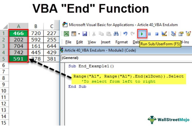
Excel vba cell end - Word и Excel - помощь в работе с программами

Свойство End объекта Range применяется для поиска первых и последних заполненных ячеек в VBA Excel — аналог сочетания клавиш Ctrl+стрелка.

Свойство End объекта Range возвращает объект Range, представляющий ячейку в конце или начале заполненной значениями области исходного диапазона по строке или столбцу в зависимости от указанного направления. Является в VBA Excel программным аналогом сочетания клавиш — Ctrl+стрелка (вверх, вниз, вправо, влево).

Возвращаемая свойством Range.End ячейка в зависимости от расположения и содержания исходной:

Исходная ячейка	Возвращаемая ячейка
Исходная ячейка пустая	Первая заполненная ячейка или, если в указанном направлении заполненных ячеек нет, последняя ячейка строки или столбца в заданном направлении.
Исходная ячейка не пустая и не крайняя внутри исходного заполненного диапазона в указанном направлении	Последняя заполненная ячейка исходного заполненного диапазона в указанном направлении
Исходная ячейка не пустая, но в указанном направлении является крайней внутри исходного заполненного диапазона	Первая заполненная ячейка следующего заполненного диапазона или, если в указанном направлении заполненных ячеек нет, последняя ячейка строки или столбца в заданном направлении.

Синтаксис

Expression.End (Direction)

Expression — выражение (переменная), представляющее объект Range.

Параметры

Параметр	Описание
Direction	Константа из коллекции `XlDirection`, задающая направление перемещения. Обязательный параметр.

Константы XlDirection:

Константа	Значение	Направление
xlDown	-4121	Вниз
xlToLeft	-4159	Влево
xlToRight	-4161	Вправо
xlUp	-4162	Вверх

Примеры

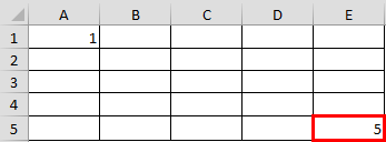
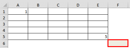
Скриншот области рабочего листа для визуализации примеров применения свойства Range.End:

Примеры возвращаемых ячеек свойством End объекта Range("C10") с разными значениями параметра Direction:

Выражение с Range.End	Возвращенная ячейка
`Set myRange = Range("C10").End(xlDown)`	`Range("C16")`
`Set myRange = Range("C10").End(xlToLeft)`	`Range("A10")`
`Set myRange = Range("C10").End(xlToRight)`	`Range("E10")`
`Set myRange = Range("C10").End(xlUp)`	`Range("C4")`

Пример возвращения заполненной значениями части столбца:

Sub Primer()

Dim myRange As Range

Set myRange = Range(Range(«C10»), Range(«C10»).End(xlDown))

MsgBox myRange.Address ‘Результат: $C$10:$C$16

End Sub

Источник

Return to VBA Code Examples

This tutorial will show you how to use the Range.End property in VBA.

Most things that you do manually in an Excel workbook or worksheet can be automated in VBA code.

If you have a range of non-blank cells in Excel, and you press Ctrl+Down Arrow, your cursor will move to the last non-blank cell in the column you are in. Similarly, if you press Ctrl+Up Arrow, your cursor will move to the first non-blank cell. The same applies for a row using the Ctrl+Right Arrow or Ctrl+Left Arrow to go to the beginning or end of that row. All of these key combinations can be used within your VBA code using the End Function.

Range End Property Syntax

The Range.End Property allows you to move to a specific cell within the Current Region that you are working with.

expression.End (Direction)

the expression is the cell address (Range) of the cell where you wish to start from eg: Range(“A1”)

END is the property of the Range object being controlled.

Direction is the Excel constant that you are able to use. There are 4 choices available – xlDown, xlToLeft, xlToRight and xlUp.

Moving to the Last Cell

The procedure below will move you to the last cell in the Current Region of cells that you are in.

Sub GoToLast()
'move to the last cell occupied in the current region of cells
   Range("A1").End(xlDown).Select
End Sub

Counting Rows

The following procedure allows you to use the xlDown constant with the Range End property to count how many rows are in your current region.

Sub GoToLastRowofRange()
   Dim rw As Integer
   Range("A1").Select
'get the last row in the current region
   rw = Range("A1").End(xlDown).Row
'show how many rows are used
   MsgBox "The last row used in this range is " & rw
End Sub

While the one below will count the columns in the range using the xlToRight constant.

Sub GoToLastCellofRange() 
   Dim col As Integer 
   Range("A1").Select 
'get the last column in the current region
   col = Range("A1").End(xlToRight).Column
'show how many columns are used
   MsgBox "The last column used in this range is " & col
 End Sub

Creating a Range Array

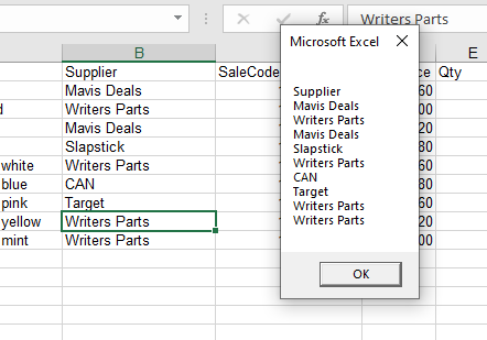
The procedure below allows us to start at the first cell in a range of cells, and then use the End(xlDown) property to find the last cell in the range of cells. We can then ReDim our array with the total rows in the Range, thereby allowing us to loop through the range of cells.

Sub PopulateArray()
'declare the array
   Dim strSuppliers() As String
'declare the integer to count the rows
   Dim n As Integer
'count the rows
   n = Range("B1", Range("B1").End(xlDown)).Rows.Count
'initialise and populate the array
   ReDim strCustomers(n)
'declare the integer for looping
   Dim i As Integer
'populate the array
   For i = 0 To n
     strCustomers(i) = Range("B1").Offset(i, 0).Value
   Next i
'show message box with values of array
   MsgBox Join(strCustomers, vbCrLf)
End Sub

When we run this procedure, it will return the following message box.

VBA Coding Made Easy

Stop searching for VBA code online. Learn more about AutoMacro — A VBA Code Builder that allows beginners to code procedures from scratch with minimal coding knowledge and with many time-saving features for all users!

Learn More!

Источник

VBA END Function

End Statement is almost used in every other programming language, so VBA is also not different from it. Every code has a start and has an end for it. How do we end any specific function or code is different in programming languages. In VBA we close our code by using END Statement. But apart from this end statement, we have another end function in VBA which is used to refer to the cells of a worksheet which we will talk about detail in this article.

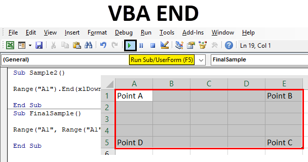
As I have told above we will be discussing another property of END in VBA which is used to refer to the end of the cells. There are many separate properties for this END function. For example, end to the right or end the left or end to the bottom. To make this more clear look at below the image.

In Excel worksheet how do we move from cell A1 which points A to cell E1 which is point B? We press CTRL + right arrow. Similarly to move from point B to point C we press CTRL + Down Arrow and from point C to point D we press CTRL + Left arrow. Similarly for point D to point A we press CTRL + Up arrow.

This is also known as to refer to the next cell which has some value in it. This process skips the blank cells and moves to the end of the reference. In VBA we do not press CTRL + Right Arrow to move from point A to point B. We use properties of END to do this. And this is what we will learn in this article. How can we move from Point A to End to the right which is point B and select the cell range and do the same for others.

How to Use VBA End Function in Excel?

We will learn how to use a VBA END Function with example in excel.

You can download this VBA END Excel Template here – VBA END Excel Template

Let us learn to do so by a few examples.

Example #1 – VBA END

In the first example let us select cell E1 using the end property in VBA.

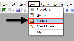
Step 1: From the Insert tab insert a new module. Remember we will work in the same module for the entire article. We can see the module in the project window, Open the module as shown below.

Module

Step 2: Start the Sub procedure in the window.

Code:

Sub sample()

End Sub

Step 3: Now we know that we have to move from cell A1 to cell E1 so type the following code.

Code:

Sub sample()

Range ("A1")

End Sub

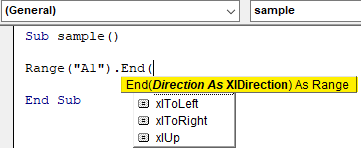
Step 4: Now put a dot after the parenthesis and write end as shown below.

Code:

Sub sample()

Range("A1").End

End Sub

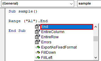
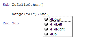
Step 5: Press Enter and open a parenthesis we will see some more options in the end statement as follows,

Code:

Sub sample()

Range("A1").End(

End Sub

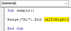
Step 6: Select XltoRight as we have to move right to select cell E1.

Code:

Sub sample()

Range("A1").End (xlToRight)

End Sub

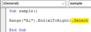
Step 7: Now to select the range, put a dot after the closing parenthesis and write select as shown below.

Code:

Sub sample()

Range("A1").End(xlToRight).Select

End Sub

Step 8: Now let us execute the code written above and see the result in sheet 1 as follows.

From Point A which is cell A1 we moved to the end of the data in the right which is cell E1.

Example #2 – VBA END

Similar to the above example where we moved right from the cell A1 we can move left too. Let us select cell A5 which is point C from Point D.

Step 1: In the same module, declare another subprocedure for another demonstration.

Code:

Sub Sample1()

End Sub

Step 2: Now let us move from cell E5 to cell A5, so first refer to cell E5 as follows.

Code:

Sub Sample1()

Range ("E5")

End Sub

Step 3: Now let us move to the left of the cell E5 using the end statement.

Code:

Sub Sample1()

Range("E5").End (xlToLeft)

End Sub

Step 4: Now to select cell A5 put a dot after the parenthesis and write select.

Code:

Sub Sample1()

Range("E5").End(xlToLeft).Select

End Sub

Step 5: Now execute this code above and see the result in sheet 1 as follows.

From point C we moved to point D using the end statement.

Example #3 – VBA END

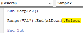
Now let use the downwards end statement which means we will select cell A5 from cell A1.

Step 1: In the same module, declare another subprocedure for another demonstration.

Code:

Sub Sample2()

End Sub

Step 2: Now let us move from cell A5 to cell A1, so first refer to cell A1 as follows.

Code:

Sub Sample2()

Range ("A1")

End Sub

Step 3: Now let us move to the down of the cell A1 using the end statement.

Code:

Sub Sample2()

Range("A1").End (xlDown)

End Sub

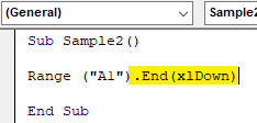
Step 4: Now to select cell A5 put a dot after the parenthesis and write select.

Code:

Sub Sample2()

Range("A1").End(xlDown).Select

End Sub

Step 5: Now execute this code above and see the result in sheet 1 as follows.

We have moved from Point A to point D using the down property of the end statement.

Example #4 – VBA END

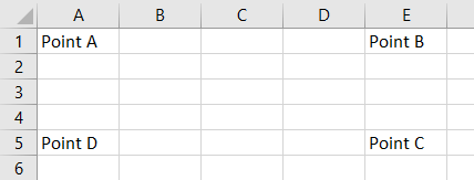
Now let us select the total range from Point A to Point B to Point C and to Point D using the end statement.

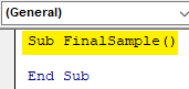
Step 1: In the same module, declare another subprocedure for another demonstration.

Code:

Sub FinalSample()

End Sub

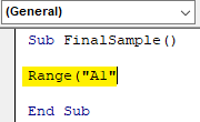
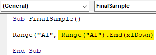
Step 2: Now let us select from cell A1 to cell E5, so first refer to cell A1 as follows.

Code:

Sub FinalSample()

Range("A1"

End Sub

Step 3: Now let us move down of the cell A1 using the end statement.

Code:

Sub FinalSample()

Range("A1", Range("A1").End(xlDown)

End Sub

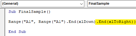
Step 4: Now we need to move to the right of the cell A1 by using the following end statement as follows.

Code:

Sub FinalSample()

Range("A1", Range("A1").End(xlDown).End(xlToRight))

End Sub

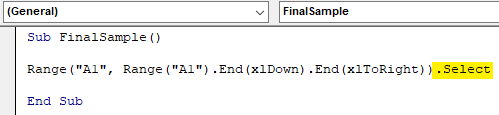
Step 5: Select the cell range using the select statement.

Code:

Sub FinalSample()

Range("A1", Range("A1").End(xlDown).End(xlToRight)).Select

End Sub

Step 6: Let us run the above code and see the final result in sheet 1 as follows.

VBA End

Things to Remember

The method to use END in VBA Excel to refer cells is very easy. We refer to a range first
Range( Cell ) and then we use End property to select or go to the last used cell in the left-right or down of the reference cell
Range (Cell).End(XltoRight) to got to the right of the cell.
First things which we need to remember is END property is different to the ending of a procedure or a function in VBA.
We can use a single property to refer to a cell i.e. to right or left of it or we can select the whole range together.
In a worksheet, we use the same reference using the CTRL button but in VBA we use the END statement.

End Function in VBA

An End is a statement in VBA that has multiple forms in VBA applications. One can put a simple End statement anywhere in the code. It will automatically stop the execution of the code. One can use the End statement in many procedures like to end the sub procedure or to end any Loop function like “End If.”

For everything, there is an end. In VBA, it is no different. You must have seen the word “End” in all the codes in your VBA. We can End in “End Sub,” “End Function,” and “End If.” These are common as we know each “End” suggests the end of the procedure. These VBA End statements do not require any special introduction because we are familiar with them in our VBA codingVBA code refers to a set of instructions written by the user in the Visual Basic Applications programming language on a Visual Basic Editor (VBE) to perform a specific task.read more.

Apart from the above “End,” we have one property, “End,” in VBA. This article will take you through that property and how to use it in our coding.

End Function in VBA
- End Property in VBA
- Examples of Excel VBA End Function
  - Example #1 – Use VBA End Property To Move in Worksheet
  - Example #2 – Selection Using End Property
  - Example #3 – Select Right to Left, Right to Bottom, & Top
- Recommended Articles

VBA End

End Property in VBA

The “End” is the property we use in VBA to move in the suggested direction. The typical example of direction is moving from the active cell to the last used cell or the last entry cell horizontally and vertically in the worksheet.

For example, let us recall this with a worksheet. Look at the below image.

Right now, we are in the A1 cell.

If we want to move to the last used cell horizontally, we use the excel shortcut keyAn Excel shortcut is a technique of performing a manual task in a quicker way.read more Ctrl + Right Arrow, which will take us to the last used cell horizontally.

Similarly, if we want to move to the last used cell downwards or vertically, we press the shortcut key Ctrl + Down Arrow.

So, to move from left to right, we press Ctrl + Left Arrow. To move from bottom to top, we press Ctrl + Up Arrow.

A similar thing can be done in VBA but not by using the Ctrl key. Rather, we need to use the word “End.”

Examples of Excel VBA End Function

You can download this VBA End Excel Template here – VBA End Excel Template

Example #1 – Use VBA End Property To Move in Worksheet

Let us look at how to use Excel VBA End to move in the sheet. First, we need to decide which cell we need to move. For example, suppose we need to move from cell A1, so refer to the cell using the VBA Range objectRange is a property in VBA that helps specify a particular cell, a range of cells, a row, a column, or a three-dimensional range. In the context of the Excel worksheet, the VBA range object includes a single cell or multiple cells spread across various rows and columns.read more.

Code:

Sub End_Example1()

  Range ("A1")

End Sub

Put dot (.) to see the IntelliSense list. Then, select “End” VBA property from the list.

Code:

Sub End_Example1()

  Range("A1").End

End Sub

Once the end property is selected, open parenthesis.

Code:

Sub End_Example1()

  Range("A1").End(

End Sub

As soon as you open parenthesis, we can see all the available options with the “End” property. Select “xlToRight” to move horizontally from cell A1 to the last used cell.

Code:

Sub End_Example1()

  Range("A1").End (xlToRight)

End Sub

After moving to the last cell, we must select what we need to do. Put dot (.) to see the IntelliSense list.

Code:

Sub End_Example1()

  Range("A1").End(xlToRight).

End Sub

Choose the “Select” method from the IntelliSense list.

Code:

Sub End_Example1()

  Range("A1").End(xlToRight).Select

End Sub

It will make use of cell A1 to last used cells horizontally.

Similarly, use the other three options to move right, left, down, and up.

To move right from cell A1.

Code:

Sub End_Example1()

  Range("A1").End(xlToRight).Select

End Sub

To move down from cell A1.

Code:

Sub End_Example1()

  Range("A1").End(xlDown).Select

End Sub

To move up from cell A5.

Code:

Sub End_Example1()

  Range("A5").End(xlUp).Select

End Sub

To move left from cell D1.

Code:

Sub End_Example1()

  Range("D1").End(xlToLeft).Select

End Sub

All the above codes are examples of using the “End” property to move in the worksheet.

We will now see how to select the ranges using the “End” property.

Example #2 – Selection Using End Property

We need to end the property to select the range of cells in the worksheet. For this example, consider the below data.

Select A1 to Last Used Cell

To select the cells from A1 to the last used cell horizontally, first, mention cell A1 in the Range object.

Code:

Sub End_Example2()

  Range("A1",

End Sub

For the second argument, open one more Range object and mention the cell as A1 only.

Code:

Sub End_Example2()

  Range("A1",Range("A1")

End Sub

Close only one bracket and put a dot to select the Excel VBA End property.

Code:

Sub End_Example2()

  Range("A1",Range("A1").End(

End Sub

Now, select xlToRight and close two brackets.

Code:

Sub End_Example2()

  Range("A1",Range("A1").End(xlToRight))

End Sub

Now, choose the “Select” method.

Code:

Sub End_Example2()

  Range("A1", Range("A1").End(xlToRight)).Select

End Sub

We have completed it now.

Run this code to see the impact.

As you can see, it has selected the range A1 to D1.

Similarly, to select downwards, use the below code.

Code:

Sub End_Example2()

  Range("A1", Range("A1").End(xlDown)).Select
     'To select from left to right
End Sub

Code:

Sub End_Example2()

  Range("A1", Range("A1").End(xlDown)).Select
     'To select from top to down
End Sub

Code:

Sub End_Example2()

  Range("D1", Range("D1").End(xlToLeft)).Select
     'To select from right to left
End Sub

Code:

Sub End_Example2()

  Range("A5", Range("A5").End(xlUp)).Select
     'To select from bottom to up
End Sub

Example #3 – Select Right to Left, Right to Bottom, & Top

We have seen how to select horizontally and vertically. Next, we need to use two “End” properties to select vertically and horizontally. For example, to select the data from A1 to D5, we need to use the below code.

Code:

Sub End_Example3()

 Range("A1", Range("A1").End(xlDown).End(xlToRight)).Select
  'To from cell A1 to last use cell downwards & rightwards
End Sub

It will select the complete range like the one below.

Like this, we can use the VBA “End” function property to select a range of cells.

Recommended Articles

This article has been a guide to the Excel VBA End function. Here, we learn how to use End property in VBA and End property selection, examples, and a downloadable template. Below are some useful Excel articles related to VBA: –

VBA Split
Call Sub in Excel
Today in VBA
How to Paste in VBA?

Источник

Хитрости »

1 Май 2011 403615 просмотров

Очень часто при внесении данных на лист Excel возникает вопрос определения последней заполненной или первой пустой ячейки. Чтобы впоследствии с этой первой пустой ячейки начать заносить данные. В этой теме я опишу несколько способов определения последней заполненной ячейки.

В качестве переменной, которой мы будем присваивать номер последней заполненной строки, у нас во всех примерах будет lLastRow. Объявлять мы её будем как Long. Для экономии памяти можно было бы использовать и тип Integer, но т.к. строк на листе может быть больше 32767(это максимальное допустимое значение переменных типа Integer) нам понадобиться именно Long, во избежание ошибки. Подробнее про типы переменных можно прочитать в статье Что такое переменная и как правильно её объявить

Одинаковые переменные для всех примеров
Во всех примерах ниже мы будем запоминать номер последней строки или столбца в одни и те же переменные:

    Dim lLastRow As Long
    'а для lLastCol можно было бы применить и тип Integer,
    'т.к. столбцов в Excel пока меньше 32767, но для однообразности назначим тоже Long
    Dim lLastCol As Long

Определение последней ячейки через свойство End

Определение последней ячейки через SpecialCells

Определение последней ячейки через UsedRange

Определение последней ячейки через метод Find

Несколько практических кодов

Способ 1:

Определение

последней заполненной строки

через свойство End

    lLastRow = Cells(Rows.Count,1).End(xlUp).Row
    'или
    lLastRow = Cells(Rows.Count, "A").End(xlUp).Row

1 или «A» — это номер или имя столбца, последнюю заполненную ячейку в котором мы определяем. По сути обе приведенные строки дадут абсолютно одинаковый результат. Просто иногда удобнее указать номер столбца, а иногда его имя. Поэтому использовать можно любой из приведенных вариантов, в зависимости от ситуации.
Определение последнего столбца через свойство End

lLastCol = Cells(1, Columns.Count).End(xlToLeft).Column

1 — это номер строки, последнюю заполненную ячейку в которой мы определяем.

Данный метод определения последней строки/столбца самый распространенный. Используя его мы можем определить последнюю ячейку только в одном конкретном столбце(или строке). В большинстве случаев этого более чем достаточно.

Метод основан именно на принципе работы свойства End. На примере поиска последней строки опишу принцип так, как бы мы это делали руками через выделение ячеек на листе:

выделили самую последнюю ячейку столбца А на листе(для Excel 2007 и выше это А1048576, а для Excel 2003 — А65536)

и выполнили переход вверх комбинацией клавиш Ctrl+стрелка вверх. Данная комбинация заставляет Excel двигаться вверх(если точнее, то в направлении стрелки, нажатой вместе с Ctrl) до тех пор, пока не встретиться первая ячейка с формулой или значением. А в случае, если сочетание было вызвано из уже заполненных ячеек — то до первой пустой. И как только Excel доходит до этой ячейки — он её выделяет

А через свойство .Row мы просто получаем номер строки этой выделенной ячейки

Нюансы:

даже если в ячейке нет видимого значения, но есть формула — End посчитает ячейку не пустой. С одной стороны вполне справедливо. Но иногда нам надо определить именно «визуально» заполненные ячейки. Поиск ячеек при подобных условиях будет описан ниже(Способ 4: Определение последней ячейки через метод Find)
если на листе заполнены все строки в просматриваемом столбце(или будут заполнены несколько последних ячеек столбца или даже только одна последняя) — то результат может быть неверный(ну или не совсем такой, какой ожидали)
Данный способ игнорирует строки, скрытые фильтром, группировкой или командой Скрыть (Hide). Т.е. если последняя строка таблицы будет скрыта, то данный метод вернет номер последней видимой заполненной строки, а не последней реально заполненной.

Ну а если надо получить первую пустую ячейку на листе(а не первую заполненную) — придется вспомнить математику. Т.к. последнюю заполненную мы определили, то первая пустая — следующая за ней. Т.е. к результату необходимо прибавить 1. Это хоть и очевидно, но на всякий случай все же лучше об этом напомнить.

Способ 2:

Определение

последней заполненной строки

через SpecialCells

    lLastRow = Cells.SpecialCells(xlLastCell).Row

Определение последнего столбца через SpecialCells

    lLastCol = Cells.SpecialCells(xlLastCell).Column

Данный метод не требует указания номера столбца и возвращает последнюю ячейку(Row — строку, Column — столбец).
Если хотите получить номер первой пустой строки или столбца на листе — к результату необходимо прибавить 1.
Нюансы:

Используя данный способ следует помнить, что не всегда можно получить реальную последнюю заполненную ячейку, т.е. именно ячейку со значением. Метод SpecialCells определяет самую «дальнюю» ячейку на листе, используя при этом механизм «запоминания» тех ячеек, в которых мы работали в данном листе. Т.е. если мы занесем в ячейку AZ90345 значение и сразу удалим его — lLastRow, полученная через SpecialCells будет равна значению именно этой ячейки, из которой вы только что удалили значения(т.е. 90345). Другими словами требует обязательного обновления данных, а этого можно добиться только сохранив файла, а временами даже только закрыв файл и открыв его снова. Так же, если какая-либо ячейка содержит форматирование(например, заливку), но не содержит никаких значений, то метод SpecialCells посчитает её используемой и будет учитывать как заполненную.
Этот недостаток можно попробовать обойти, вызвав перед определением последней ячейки вот такую строку кода:
```
With ActiveSheet.UsedRange: End With
```
Это должно переопределить границы рабочего диапазона и тогда определение последней строки/столбца сработает как ожидается, даже если до этого в ячейке содержались данные, которые впоследствии были удалены.
Выглядеть в единой процедуре это будет так:
```
Sub GetLastCell()
    Dim lLastRow As Long
    'переопределяем рабочий диапазон листа
    With ActiveSheet.UsedRange: End With
    'ищем последнюю заполненную ячейку на листе
    lLastRow = Cells.SpecialCells(xlLastCell).Row
End Sub
```
даже если в ячейке нет видимого значения, но есть формула — SpecialCells посчитает ячейку не пустой
Данный метод определения последней ячейки не будет работать на защищенном листе(Рецензирование(Review) —Защитить лист(Protect Sheet)).
Данный метод не будет работать при использовании внутри UDF. Точнее будет работать не так, как ожидается. Подробнее про некоторые «баги» работы встроенных методов внутри UDF(функций пользователя) я описывал в этой статье: Глюк работы в UDF методов SpecialCells и FindNext

Сам же я этот метод обычно использую для определения последней ячейки в только что созданном файле, в котором только добавляю строки кодом и в котором не может быть описанных выше нюансов.

Способ 3:
Определение последней строки через UsedRange

    lLastRow = ActiveSheet.UsedRange.Row + ActiveSheet.UsedRange.Rows.Count - 1

Определение последнего столбца через UsedRange

    lLastCol = ActiveSheet.UsedRange.Column + ActiveSheet.UsedRange.Columns.Count - 1

НЕМНОГО ПОЯСНЕНИЙ:

ActiveSheet.UsedRange.Row — этой строкой мы определяем первую ячейку, с которой начинаются данные на листе. Важно понимать для чего это — если у вас первые строк 5 не заполнены ничем(т.е. самые первые данные заносились начиная с 6-ой строки листа), то ActiveSheet.UsedRange.Row вернет именно 6(т.е. номер первой строки с данными). Если же все строки заполнены — то вернет 1.
ActiveSheet.UsedRange.Rows.Count — определяем кол-во строк, входящих в весь диапазон данных на листе. При этом неважно, есть ли данные в ячейках или нет — достаточно было поработать в этих ячейках и удалить значения или просто изменить цвет заливки.
В итоге получается: первая строка данных + кол-во строк с данными — 1. Зачем вычитать единицу? Попробуем посчитать вместе: первая строка: 6. Всего строк: 3. 6 + 3 = 9. Вроде все верно. А теперь выделим на листе три ячейки, начиная с 6-ой. Выделение завершилось на 8-ой строке. Потому что в 6-ой строке уже есть данные. Поэтому и надо вычесть 1, чтобы учесть этот момент. Думаю, не надо пояснять, что если надо получить первую пустую ячейку — можно 1 не вычитать
То же самое и с ActiveSheet.UsedRange.Column, только уже не для строк, а для столбцов.

Нюансы:

Обладает некоторыми недостатками предыдущего метода. Определяет самую «дальнюю» ячейку на листе, используя при этом механизм «запоминания» тех ячеек, в которых мы работали в данном листе. Следовательно попробовать обойти этот момент можно точно так же: перед определением последней строки/столбца записать строку: With ActiveSheet.UsedRange: End With
Это должно переопределить границы рабочего диапазона и тогда определение последней строки/столбца сработает как ожидается, даже если до этого в ячейке содержались данные, которые впоследствии были удалены.
даже если в ячейке нет видимого значения, но есть формула — UsedRange посчитает ячейку не пустой

Однако метод через UsedRange.Row работает прекрасно и при установленной на лист защите и внутри UDF, что делает его более предпочтительным, чем метод через SpecialCells при равных условиях.

Способ 4:
Определение последней строки и столбца, а так же адрес ячейки методом Find

Sub GetLastCell_Find()
    Dim rF As Range
    Dim lLastRow As Long, lLastCol As Long
    'ищем последнюю ячейку на листе, в которой хранится хоть какое-то значение
    Set rF = ActiveSheet.UsedRange.Find(What:="*", LookIn:=xlValues, LookAt:=xlWhole, SearchDirection:=xlPrevious, MatchCase:=False, MatchByte:=False)
    If Not rF Is Nothing Then
        lLastRow = rF.Row    'последняя заполненная строка
        lLastCol = rF.Column 'последний заполненный столбец
        MsgBox rF.Address 'показываем сообщение с адресом последней ячейки
    Else
        'если ничего не нашлось - значит лист пустой
        'и можно назначить в качестве последних первую строку и столбец
        lLastRow = 1
        lLastCol = 1
        MsgBox "A1" 'показываем сообщение с адресом ячейки А1
    End If
End Sub

Этот метод, пожалуй, самый оптимальный в случае, если надо определить последнюю строку/столбец на листе без учета форматов и формул — только по отображаемому значению в ячейке. Например, если на листе большая таблица и последние строки заполнены формулами, возвращающими при определенных условиях пустую ячейку(=ЕСЛИ(A1>0;1;»»)), предыдущие варианты вернут строку/столбец ячейки с последней ячейкой, в которой формула. В то время как данный метод вернет адрес ячейки только в случае, если в ячейке реально отображается какое-то значение. Такой подход часто используется для того, чтобы определить границы данных для последующего анализа заполненных данных, чтобы не захватывать пустые ячейки с формулами и не тратить время на их проверку.
Здесь следует обратить внимание на параметры метода Find. В данном случае мы специально указываем искать по значениям, а не по формулам:
Set rF = ActiveSheet.UsedRange.Find(What:=»*», LookIn:=xlValues, LookAt:=xlWhole, SearchDirection:=xlPrevious, MatchCase:=False, MatchByte:=False)
Нюансы:

Метод Find, вызванный с листа или другим кодом, имеет свойство запоминать все параметры последнего поиска, а если поиск еще не вызывался — то применяются параметры по умолчанию. А по умолчанию поиск идет всегда по формулам. Поэтому я настоятельно рекомендую указывать принудительно все необходимые параметры, как в примере.
Метод Find не будет учитывать в просмотре скрытые строки и столбцы. Это следует учитывать при его применении.

Пара небольших практических кодов

Коды ниже могут помочь понять, как использовать приведенные выше строки кода по поиску последней ячейки/строки:

Sub GetLastCell()
    Dim lLastRow As Long
    Dim lLastCol As Long
    'определили последнюю заполненную ячейку с учетом формул в столбце А
    lLastRow = Cells(Rows.Count, 1).End(xlUp).Row
    MsgBox "Заполненные ячейки в столбце А: " & Range("A1:A" & lLastRow).Address
    'определили последний заполненный столбец на листе(с учетом формул и форматирования)
    lLastCol = Cells.SpecialCells(xlLastCell).Column
    MsgBox "Заполненные ячейки в первой строке: " & Range(Cells(1, 1), Cells(1, lLastCol)).Address
    'выводим сообщение с адресом последней ячейки на листе(с учетом формул и форматирования)
    MsgBox "Адрес последней ячейки диапазона на листе: " & Cells.SpecialCells(xlLastCell).Address
End Sub

Выделяем диапазон ячеек в столбцах с А по С, определяя последнюю ячейку по столбцу A этого же листа:

Sub SelectToLastCell()
    Range("A1:C" & Cells(Rows.Count, 1).End(xlUp).Row).Select
End Sub

Копируем ячейку B1 в первую пустую ячейку столбца A этого же листа:

Sub CopyToFstEmptyCell()
    Dim lLastRow As Long
    lLastRow = Cells(Rows.Count, 1).End(xlUp).Row 'определили последнюю заполненную ячейку
    Range("B1").Copy Cells(lLastRow+1, 1)         'скопировали В1 и вставили в следующую после определенной ячейки
End Sub

А код ниже делает тоже самое, но одной строкой — применяется Offset и используется тот факт, что изначально методом End мы получаем именно ячейку, а не номер строки(номер строки мы получаем позже через свойство .Row):

Sub CopyToFstEmptyCell()
    Range("B1").Copy Destination:=Cells(Rows.Count, 1).End(xlUp).Offset(1)
End Sub

Range(«B1»).Copy — копирует ячейку В1. Если для аргумента Destination указать другую ячейку, то в неё будет вставлена скопированная ячейка. Мы передаем в этот аргумент определенную методом End ячейку
Cells(Rows.Count, 1).End(xlUp) — возвращает последнюю заполненную ячейку в столбце А (не строку, а именно ячейку)
Offset(1) — смещает полученную ячейку на строку вниз
Используем инструмент автозаполнение(протягивание) столбца В, начиная с ячейки B2 и определяя последнюю ячейку для заполнения на основании столбца А

Sub AutoFill_B()
    Dim lLastRow As Long
    lLastRow = Cells(Rows.Count, 1).End(xlUp).Row
    Range("B2").AutoFill Destination:=Range("B2:B" & lLastRow)
End Sub

На самом деле практических кодов может быть куда больше, т.к. определение последней заполненной или первой пустой ячейки является чуть ли не самой распространенной задачей при написании кодов в Excel.

Так же см.:
Как получить последнюю заполненную ячейку формулой?
Как определить первую заполненную ячейку на листе?
Что такое переменная и как правильно её объявить?

Статья помогла? Поделись ссылкой с друзьями!

Видеоуроки

Поиск по меткам

Access
apple watch
Multex
Power Query и Power BI
VBA управление кодами
Бесплатные надстройки
Дата и время
Записки
ИП
Надстройки
Печать
Политика Конфиденциальности
Почта
Программы
Работа с приложениями
Разработка приложений
Росстат
Тренинги и вебинары
Финансовые
Форматирование
Функции Excel
акции MulTEx
ссылки
статистика

Источник

Продолжаем наш разговор про объект Excel Range, начатый в первой части. Разберём ещё несколько типовых задач и одну развлекательную. Кстати, в процессе написания второй части я дополнил и расширил первую, поэтому рекомендую её посмотреть ещё раз.

Примеры кода

Скачать

Типовые задачи

Перебор ячеек диапазона (вариант 4)

Для коллекции добавил четвёртый вариант перебора ячеек. Как видите, можно выбирать, как перебирается диапазон — по столбцам или по строкам. Обратите внимание на использование свойства коллекции Cells. Не путайте: свойство Cells рабочего листа содержит все ячейки листа, а свойство Cells диапазона (Range) содержит ячейки только этого диапазона. В данном случае мы получаем все ячейки столбца или строки.
```
Sub Handle_Cells_4_by_Columns(parRange As Range)
  For Each columnTemp In parRange.Columns
    For Each cellTemp In columnTemp.Cells
      Sum = Sum + cellTemp
    Next
  Next
  MsgBox "Сумма ячеек " & Sum
End Sub

Sub Handle_Cells_4_by_Rows(parRange As Range)
  For Each rowTemp In parRange.Rows
    For Each cellTemp In rowTemp.Cells
      Sum = Sum + cellTemp
    Next
  Next
  MsgBox "Сумма ячеек " & Sum
End Sub
 
```
Должен вас предупредить, что код, который вы видите в этом цикле статей — это код, написанный для целей демонстрации работы с объектной моделью Excel. Тут нет объявлений переменных, обработки ошибок и проверки условий, так как я специально минимизирую программы, пытаясь акцентировать ваше внимание целиком на обсуждаемом предмете — объекте Range.
Работа с текущей областью

Excel умеет автоматически определять текущую область вокруг активной ячейки. Соответствующая команда на листе вызывается через Ctrl+A. Через ActiveCell мы посредством свойства Worksheet легко выходим на лист текущей ячейки, а уже через него можем эксплуатировать свойство UsedRange, которое и является ссылкой на Range текущей области. Чтобы понять, какой диапазон мы получили, мы меняем цвет ячеек. Функция GetRandomColor не является стандартной, она определена в модуле файла примера.
```
ActiveCell.Worksheet.UsedRange.Interior.Color = GetRandomColor
 
```
Определение границ текущей области

Демонстрируем определение левого верхнего и правого нижнего углов диапазона текущей области. С левым верхним углом всё просто, так как координаты этой ячейки всегда доступны через свойства Row и Column объекта Range (не путать с коллекциями Rows и Columns!). А вот для определения второго угла приходится использовать конструкцию вида .Rows(.Rows.Count).Row, где .Rows.Count — количество строк в диапазоне UsedRange, .Rows(.Rows.Count) — это мы получили последнюю строку, и уже для этого диапазона забираем из свойства Row координату строки. Со столбцом — по аналогии. Также обратите внимание на использование оператора With. Как видите, оператор With, помимо сокращения кода, также позволяет отказаться от объявления отдельной объектной переменной через оператор Set, что очень удобно.
```
With ActiveCell.Worksheet.UsedRange
  strTemp = "Верхняя строка " & vbTab & .Row & vbCr & _
            "Нижняя строка " & vbTab & .Rows(.Rows.Count).Row & vbCr & _
            "Левый столбец " & vbTab & .Column & vbCr & _
            "Правый столбец " & vbTab & .Columns(.Columns.Count).Column
End With
MsgBox strTemp, vbInformation
 
```
Выделение столбцов / строк текущей области

Тут нет ничего нового, мы всё это обсудили в предыдущем примере. Мы получаем ссылки на столбцы / строки, меняя их цвет для контроля результата работы кода.
```
With ActiveCell.Worksheet.UsedRange
  .Rows(1).Interior.Color = GetRandomColor
  .Rows(.Rows.Count).Interior.Color = GetRandomColor
End With
 
```
```
With ActiveCell.Worksheet.UsedRange
  .Columns(1).Interior.Color = GetRandomColor
  .Columns(.Columns.Count).Interior.Color = GetRandomColor
End With
 
```
Сброс форматирования диапазона

Для возвращения диапазона к каноническому стерильному состоянию очень просто и удобно использовать свойство Style, и присвоить ему имя стиля «Normal». Интересно, что все остальные стандартные стили в локализованном офисе имеют русские имена, а у этого стиля оставили англоязычное имя, что неплохо.
```
ActiveCell.Worksheet.UsedRange.Style = "Normal"
 
```
Поиск последней строки столбца (вариант 1)

Range имеет 2 свойства EntireColumn и EntireRow, возвращающие столбцы / строки, на которых расположился ваш диапазон, но возвращают их ЦЕЛИКОМ. То есть, если вы настроили диапазон на D5, то Range(«D5»).EntireColumn вернёт вам ссылку на D:D, а EntireRow — на 5:5.

Идём далее — свойство End возвращает вам ближайшую ячейку в определенном направлении, стоящую на границе непрерывного диапазона с данными. Как это работает вы можете увидеть, нажимая на листе комбинации клавиш Ctrl+стрелки. Кстати, это одна из самых полезных горячих клавиш в Excel. Направление задаётся стандартными константами xlUp, xlDown, xlToRight, xlToLeft.

Классическая задача у Excel программиста — определить, где кончается таблица или, в данном случае, конкретный столбец. Идея состоит в том, чтобы встать на последнюю ячейку столбца (строка 1048576) и, стоя в этой ячейке, перейти по Ctrl+стрелка вверх (что на языке VBA — End(xlUp)).
```
With ActiveCell.EntireColumn
  .Cells(.Rows.Count, 1).End(xlUp).Select
End With
 
```
Поиск последней строки столбца (вариант 2)

Ещё один вариант.
```
With ActiveCell.Worksheet
  .Cells(.Rows.Count, ActiveCell.Column).End(xlUp).Select
End With
 
```
Поиск «последней» ячейки листа

Тут показывается, как найти на листе ячейку, ниже и правее которой находятся только пустые ячейки. Соответственно данные надо искать в диапазоне от A1 до этой ячейки. На эту ячейку можно перейти через Ctrl+End. Как этим воспользоваться в VBA показано ниже:
```
ActiveCell.Worksheet.Cells.SpecialCells(xlCellTypeLastCell).Select
 
```

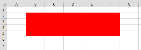
Разбор клипо-генератора

Ну, и в качестве развлечения и разрядки взгляните на код клипо-генератора, который генерирует цветные квадраты в заданных границах экрана. На некоторых это оказывает умиротворяющий эффект

По нашей теме в коде обращает на себя внимание использование свойства ReSize объекта Range. Как не трудно догадаться, свойство расширяет (усекает) текущий диапазон до указанных границ, при этом левый верхний угол диапазона сохраняет свои координаты. А также посмотрите на 2 последние строчки кода, реализующие очистку экрана. Там весьма показательно использован каскад свойств End и Offset.

Sub Indicator(start As Range)

  ' выясняем границы "экрана" (чёрная рамка с ячейками =1)
  LimitUp = start.End(xlUp).Row
  LimitDown = start.End(xlDown).Row
  LimitRight = start.End(xlToRight).Column
  LimitLeft = start.End(xlToLeft).Column
  
  ' бесконечный цикл, пока пользователь не нажал кнопку "Стоп"
  Do While Not PleaseStop
  
    ' размер клипа может меняться счётчиком, поэтому обновляем из ИД
    MinSize = Range("rngSize")
  
    iColor = GetRandomColor ' получаем случайный цвет для "клипа"
  
    ' верхний угол "клипа"
    iTop = LimitUp + Int(Rnd * (LimitDown - LimitUp - MinSize)) + 1
    
    ' левый угол "клипа"
    iLeft = LimitLeft + Int(Rnd * (LimitRight - LimitLeft - MinSize)) + 1
    
    ' выводим "клип" на экран, закрашивая фон диапазона
    ' размер диапазона - квадрат со стороной MinSize
    Cells(iTop, iLeft).Resize(MinSize, MinSize).Interior.Color = iColor
    
    ' Задержка между клипами зависит от MinSize, 5 - в миллисекундах
    Sleep 5 * MinSize
    
    DoEvents ' даём операционной системе и приложениям нормально функционировать
    
  Loop
  
  ' после завершения цикла переходим в верхний левый угол экрана
  start.End(xlUp).End(xlToLeft).Offset(1, 1).Select
  ' выделяем "экран" и очищаем его через изменния стиля ячеек
  Range(Selection, Selection.End(xlToRight).End(xlDown).Offset(-1, -1)).Style = "Normal"
  
End Sub

A Quick Guide to Ranges and Cells

Function	Takes	Returns	Example	Gives
Range	cell address	multiple cells	.Range(«A1:A4»)	$A$1:$A$4
Cells	row, column	one cell	.Cells(1,5)	$E$1
Offset	row, column	multiple cells	Range(«A1:A2») .Offset(1,2)	$C$2:$C$3
Rows	row(s)	one or more rows	.Rows(4) .Rows(«2:4»)	$4:$4 $2:$4
Columns	column(s)	one or more columns	.Columns(4) .Columns(«B:D»)	$D:$D $B:$D

Download the Code

The Webinar

If you are a member of the VBA Vault, then click on the image below to access the webinar and the associated source code.

(Note: Website members have access to the full webinar archive.)

Introduction

This is the third post dealing with the three main elements of VBA. These three elements are the Workbooks, Worksheets and Ranges/Cells. Cells are by far the most important part of Excel. Almost everything you do in Excel starts and ends with Cells.

Generally speaking, you do three main things with Cells

Read from a cell.
Write to a cell.
Change the format of a cell.

Excel has a number of methods for accessing cells such as Range, Cells and Offset.These can cause confusion as they do similar things and can lead to confusion

In this post I will tackle each one, explain why you need it and when you should use it.

Let’s start with the simplest method of accessing cells – using the Range property of the worksheet.

Important Notes

I have recently updated this article so that is uses Value2.

You may be wondering what is the difference between Value, Value2 and the default:

' Value2
Range("A1").Value2 = 56

' Value
Range("A1").Value = 56

' Default uses value
Range("A1") = 56

Using Value may truncate number if the cell is formatted as currency. If you don’t use any property then the default is Value.

It is better to use Value2 as it will always return the actual cell value(see this article from Charle Williams.)

The Range Property

The worksheet has a Range property which you can use to access cells in VBA. The Range property takes the same argument that most Excel Worksheet functions take e.g. “A1”, “A3:C6” etc.

The following example shows you how to place a value in a cell using the Range property.

' https://excelmacromastery.com/
Public Sub WriteToCell()

    ' Write number to cell A1 in sheet1 of this workbook
    ThisWorkbook.Worksheets("Sheet1").Range("A1").Value2 = 67

    ' Write text to cell A2 in sheet1 of this workbook
    ThisWorkbook.Worksheets("Sheet1").Range("A2").Value2 = "John Smith"

    ' Write date to cell A3 in sheet1 of this workbook
    ThisWorkbook.Worksheets("Sheet1").Range("A3").Value2 = #11/21/2017#

End Sub

As you can see Range is a member of the worksheet which in turn is a member of the Workbook. This follows the same hierarchy as in Excel so should be easy to understand. To do something with Range you must first specify the workbook and worksheet it belongs to.

For the rest of this post I will use the code name to reference the worksheet.

The following code shows the above example using the code name of the worksheet i.e. Sheet1 instead of ThisWorkbook.Worksheets(“Sheet1”).

' https://excelmacromastery.com/
Public Sub UsingCodeName()

    ' Write number to cell A1 in sheet1 of this workbook
    Sheet1.Range("A1").Value2 = 67

    ' Write text to cell A2 in sheet1 of this workbook
    Sheet1.Range("A2").Value2 = "John Smith"

    ' Write date to cell A3 in sheet1 of this workbook
    Sheet1.Range("A3").Value2 = #11/21/2017#

End Sub

You can also write to multiple cells using the Range property

' https://excelmacromastery.com/
Public Sub WriteToMulti()

    ' Write number to a range of cells
    Sheet1.Range("A1:A10").Value2 = 67

    ' Write text to multiple ranges of cells
    Sheet1.Range("B2:B5,B7:B9").Value2 = "John Smith"

End Sub

You can download working examples of all the code from this post from the top of this article.

The Cells Property of the Worksheet

The worksheet object has another property called Cells which is very similar to range. There are two differences

Cells returns a range of one cell only.
Cells takes row and column as arguments.

The example below shows you how to write values to cells using both the Range and Cells property

' https://excelmacromastery.com/
Public Sub UsingCells()

    ' Write to A1
    Sheet1.Range("A1").Value2 = 10
    Sheet1.Cells(1, 1).Value2  = 10

    ' Write to A10
    Sheet1.Range("A10").Value2 = 10
    Sheet1.Cells(10, 1).Value2  = 10

    ' Write to E1
    Sheet1.Range("E1").Value2 = 10
    Sheet1.Cells(1, 5).Value2  = 10

End Sub

You may be wondering when you should use Cells and when you should use Range. Using Range is useful for accessing the same cells each time the Macro runs.

For example, if you were using a Macro to calculate a total and write it to cell A10 every time then Range would be suitable for this task.

Using the Cells property is useful if you are accessing a cell based on a number that may vary. It is easier to explain this with an example.

In the following code, we ask the user to specify the column number. Using Cells gives us the flexibility to use a variable number for the column.

' https://excelmacromastery.com/
Public Sub WriteToColumn()

    Dim UserCol As Integer
    
    ' Get the column number from the user
    UserCol = Application.InputBox(" Please enter the column...", Type:=1)
    
    ' Write text to user selected column
    Sheet1.Cells(1, UserCol).Value2 = "John Smith"

End Sub

In the above example, we are using a number for the column rather than a letter.

To use Range here would require us to convert these values to the letter/number cell reference e.g. “C1”. Using the Cells property allows us to provide a row and a column number to access a cell.

Sometimes you may want to return more than one cell using row and column numbers. The next section shows you how to do this.

Using Cells and Range together

As you have seen you can only access one cell using the Cells property. If you want to return a range of cells then you can use Cells with Ranges as follows

' https://excelmacromastery.com/
Public Sub UsingCellsWithRange()

    With Sheet1
        ' Write 5 to Range A1:A10 using Cells property
        .Range(.Cells(1, 1), .Cells(10, 1)).Value2 = 5

        ' Format Range B1:Z1 to be bold
        .Range(.Cells(1, 2), .Cells(1, 26)).Font.Bold = True

    End With

End Sub

As you can see, you provide the start and end cell of the Range. Sometimes it can be tricky to see which range you are dealing with when the value are all numbers. Range has a property called Address which displays the letter/ number cell reference of any range. This can come in very handy when you are debugging or writing code for the first time.

In the following example we print out the address of the ranges we are using:

' https://excelmacromastery.com/
Public Sub ShowRangeAddress()

    ' Note: Using underscore allows you to split up lines of code
    With Sheet1

        ' Write 5 to Range A1:A10 using Cells property
        .Range(.Cells(1, 1), .Cells(10, 1)).Value2 = 5
        Debug.Print "First address is : " _
            + .Range(.Cells(1, 1), .Cells(10, 1)).Address

        ' Format Range B1:Z1 to be bold
        .Range(.Cells(1, 2), .Cells(1, 26)).Font.Bold = True
        Debug.Print "Second address is : " _
            + .Range(.Cells(1, 2), .Cells(1, 26)).Address

    End With

End Sub

In the example I used Debug.Print to print to the Immediate Window. To view this window select View->Immediate Window(or Ctrl G)

You can download all the code for this post from the top of this article.

The Offset Property of Range

Range has a property called Offset. The term Offset refers to a count from the original position. It is used a lot in certain areas of programming. With the Offset property you can get a Range of cells the same size and a certain distance from the current range. The reason this is useful is that sometimes you may want to select a Range based on a certain condition. For example in the screenshot below there is a column for each day of the week. Given the day number(i.e. Monday=1, Tuesday=2 etc.) we need to write the value to the correct column.

We will first attempt to do this without using Offset.

' https://excelmacromastery.com/
' This sub tests with different values
Public Sub TestSelect()

    ' Monday
    SetValueSelect 1, 111.21
    ' Wednesday
    SetValueSelect 3, 456.99
    ' Friday
    SetValueSelect 5, 432.25
    ' Sunday
    SetValueSelect 7, 710.17

End Sub

' Writes the value to a column based on the day
Public Sub SetValueSelect(lDay As Long, lValue As Currency)

    Select Case lDay
        Case 1: Sheet1.Range("H3").Value2 = lValue
        Case 2: Sheet1.Range("I3").Value2 = lValue
        Case 3: Sheet1.Range("J3").Value2 = lValue
        Case 4: Sheet1.Range("K3").Value2 = lValue
        Case 5: Sheet1.Range("L3").Value2 = lValue
        Case 6: Sheet1.Range("M3").Value2 = lValue
        Case 7: Sheet1.Range("N3").Value2 = lValue
    End Select

End Sub

As you can see in the example, we need to add a line for each possible option. This is not an ideal situation. Using the Offset Property provides a much cleaner solution

' https://excelmacromastery.com/
' This sub tests with different values
Public Sub TestOffset()

    DayOffSet 1, 111.01
    DayOffSet 3, 456.99
    DayOffSet 5, 432.25
    DayOffSet 7, 710.17

End Sub

Public Sub DayOffSet(lDay As Long, lValue As Currency)

    ' We use the day value with offset specify the correct column
    Sheet1.Range("G3").Offset(, lDay).Value2 = lValue

End Sub

As you can see this solution is much better. If the number of days in increased then we do not need to add any more code. For Offset to be useful there needs to be some kind of relationship between the positions of the cells. If the Day columns in the above example were random then we could not use Offset. We would have to use the first solution.

One thing to keep in mind is that Offset retains the size of the range. So .Range(“A1:A3”).Offset(1,1) returns the range B2:B4. Below are some more examples of using Offset

' https://excelmacromastery.com/
Public Sub UsingOffset()

    ' Write to B2 - no offset
    Sheet1.Range("B2").Offset().Value2 = "Cell B2"

    ' Write to C2 - 1 column to the right
    Sheet1.Range("B2").Offset(, 1).Value2 = "Cell C2"

    ' Write to B3 - 1 row down
    Sheet1.Range("B2").Offset(1).Value2 = "Cell B3"

    ' Write to C3 - 1 column right and 1 row down
    Sheet1.Range("B2").Offset(1, 1).Value2 = "Cell C3"

    ' Write to A1 - 1 column left and 1 row up
    Sheet1.Range("B2").Offset(-1, -1).Value2 = "Cell A1"

    ' Write to range E3:G13 - 1 column right and 1 row down
    Sheet1.Range("D2:F12").Offset(1, 1).Value2 = "Cells E3:G13"

End Sub

Using the Range CurrentRegion

CurrentRegion returns a range of all the adjacent cells to the given range.

In the screenshot below you can see the two current regions. I have added borders to make the current regions clear.

A row or column of blank cells signifies the end of a current region.

You can manually check the CurrentRegion in Excel by selecting a range and pressing Ctrl + Shift + *.

If we take any range of cells within the border and apply CurrentRegion, we will get back the range of cells in the entire area.

For example
Range(“B3”).CurrentRegion will return the range B3:D14
Range(“D14”).CurrentRegion will return the range B3:D14
Range(“C8:C9”).CurrentRegion will return the range B3:D14
and so on

How to Use

We get the CurrentRegion as follows

' Current region will return B3:D14 from above example
Dim rg As Range
Set rg = Sheet1.Range("B3").CurrentRegion

Read Data Rows Only

Read through the range from the second row i.e.skipping the header row

' Current region will return B3:D14 from above example
Dim rg As Range
Set rg = Sheet1.Range("B3").CurrentRegion

' Start at row 2 - row after header
Dim i As Long
For i = 2 To rg.Rows.Count
    ' current row, column 1 of range
    Debug.Print rg.Cells(i, 1).Value2
Next i

Remove Header

Remove header row(i.e. first row) from the range. For example if range is A1:D4 this will return A2:D4

' Current region will return B3:D14 from above example
Dim rg As Range
Set rg = Sheet1.Range("B3").CurrentRegion

' Remove Header
Set rg = rg.Resize(rg.Rows.Count - 1).Offset(1)

' Start at row 1 as no header row
Dim i As Long
For i = 1 To rg.Rows.Count
    ' current row, column 1 of range
    Debug.Print rg.Cells(i, 1).Value2
Next i

Using Rows and Columns as Ranges

If you want to do something with an entire Row or Column you can use the Rows or Columns property of the Worksheet. They both take one parameter which is the row or column number you wish to access

' https://excelmacromastery.com/
Public Sub UseRowAndColumns()

    ' Set the font size of column B to 9
    Sheet1.Columns(2).Font.Size = 9

    ' Set the width of columns D to F
    Sheet1.Columns("D:F").ColumnWidth = 4

    ' Set the font size of row 5 to 18
    Sheet1.Rows(5).Font.Size = 18

End Sub

Using Range in place of Worksheet

You can also use Cells, Rows and Columns as part of a Range rather than part of a Worksheet. You may have a specific need to do this but otherwise I would avoid the practice. It makes the code more complex. Simple code is your friend. It reduces the possibility of errors.

The code below will set the second column of the range to bold. As the range has only two rows the entire column is considered B1:B2

' https://excelmacromastery.com/
Public Sub UseColumnsInRange()

    ' This will set B1 and B2 to be bold
    Sheet1.Range("A1:C2").Columns(2).Font.Bold = True

End Sub

You can download all the code for this post from the top of this article.

Reading Values from one Cell to another

In most of the examples so far we have written values to a cell. We do this by placing the range on the left of the equals sign and the value to place in the cell on the right. To write data from one cell to another we do the same. The destination range goes on the left and the source range goes on the right.

The following example shows you how to do this:

' https://excelmacromastery.com/
Public Sub ReadValues()

    ' Place value from B1 in A1
    Sheet1.Range("A1").Value2 = Sheet1.Range("B1").Value2

    ' Place value from B3 in sheet2 to cell A1
    Sheet1.Range("A1").Value2 = Sheet2.Range("B3").Value2

    ' Place value from B1 in cells A1 to A5
    Sheet1.Range("A1:A5").Value2 = Sheet1.Range("B1").Value2

    ' You need to use the "Value" property to read multiple cells
    Sheet1.Range("A1:A5").Value2 = Sheet1.Range("B1:B5").Value2

End Sub

As you can see from this example it is not possible to read from multiple cells. If you want to do this you can use the Copy function of Range with the Destination parameter

' https://excelmacromastery.com/
Public Sub CopyValues()

    ' Store the copy range in a variable
    Dim rgCopy As Range
    Set rgCopy = Sheet1.Range("B1:B5")

    ' Use this to copy from more than one cell
    rgCopy.Copy Destination:=Sheet1.Range("A1:A5")

    ' You can paste to multiple destinations
    rgCopy.Copy Destination:=Sheet1.Range("A1:A5,C2:C6")

End Sub

The Copy function copies everything including the format of the cells. It is the same result as manually copying and pasting a selection. You can see more about it in the Copying and Pasting Cells section.

Using the Range.Resize Method

When copying from one range to another using assignment(i.e. the equals sign), the destination range must be the same size as the source range.

Using the Resize function allows us to resize a range to a given number of rows and columns.

For example:

' https://excelmacromastery.com/
Sub ResizeExamples()
 
    ' Prints A1
    Debug.Print Sheet1.Range("A1").Address

    ' Prints A1:A2
    Debug.Print Sheet1.Range("A1").Resize(2, 1).Address

    ' Prints A1:A5
    Debug.Print Sheet1.Range("A1").Resize(5, 1).Address
    
    ' Prints A1:D1
    Debug.Print Sheet1.Range("A1").Resize(1, 4).Address
    
    ' Prints A1:C3
    Debug.Print Sheet1.Range("A1").Resize(3, 3).Address
    
End Sub

When we want to resize our destination range we can simply use the source range size.

In other words, we use the row and column count of the source range as the parameters for resizing:

' https://excelmacromastery.com/
Sub Resize()

    Dim rgSrc As Range, rgDest As Range
    
    ' Get all the data in the current region
    Set rgSrc = Sheet1.Range("A1").CurrentRegion

      ' Get the range destination
    Set rgDest = Sheet2.Range("A1")
    Set rgDest = rgDest.Resize(rgSrc.Rows.Count, rgSrc.Columns.Count)
    
    rgDest.Value2 = rgSrc.Value2

End Sub

We can do the resize in one line if we prefer:

' https://excelmacromastery.com/
Sub ResizeOneLine()

    Dim rgSrc As Range
    
    ' Get all the data in the current region
    Set rgSrc = Sheet1.Range("A1").CurrentRegion
    
    With rgSrc
        Sheet2.Range("A1").Resize(.Rows.Count, .Columns.Count).Value2 = .Value2
    End With
    
End Sub

Reading Values to variables

We looked at how to read from one cell to another. You can also read from a cell to a variable. A variable is used to store values while a Macro is running. You normally do this when you want to manipulate the data before writing it somewhere. The following is a simple example using a variable. As you can see the value of the item to the right of the equals is written to the item to the left of the equals.

' https://excelmacromastery.com/
Public Sub UseVariables()

    ' Create
    Dim number As Long

    ' Read number from cell
    number = Sheet1.Range("A1").Value2

    ' Add 1 to value
    number = number + 1

    ' Write new value to cell
    Sheet1.Range("A2").Value2 = number

End Sub

To read text to a variable you use a variable of type String:

' https://excelmacromastery.com/
Public Sub UseVariableText()

    ' Declare a variable of type string
    Dim text As String

    ' Read value from cell
    text = Sheet1.Range("A1").Value2

    ' Write value to cell
    Sheet1.Range("A2").Value2 = text

End Sub

You can write a variable to a range of cells. You just specify the range on the left and the value will be written to all cells in the range.

' https://excelmacromastery.com/
Public Sub VarToMulti()

    ' Read value from cell
    Sheet1.Range("A1:B10").Value2 = 66

End Sub

You cannot read from multiple cells to a variable. However you can read to an array which is a collection of variables. We will look at doing this in the next section.

How to Copy and Paste Cells

If you want to copy and paste a range of cells then you do not need to select them. This is a common error made by new VBA users.

Note: We normally use Range.Copy when we want to copy formats, formulas, validation. If we want to copy values it is not the most efficient method.
I have written a complete guide to copying data in Excel VBA here.

You can simply copy a range of cells like this:

Range("A1:B4").Copy Destination:=Range("C5")

Using this method copies everything – values, formats, formulas and so on. If you want to copy individual items you can use the PasteSpecial property of range.

It works like this

Range("A1:B4").Copy
Range("F3").PasteSpecial Paste:=xlPasteValues
Range("F3").PasteSpecial Paste:=xlPasteFormats
Range("F3").PasteSpecial Paste:=xlPasteFormulas

The following table shows a full list of all the paste types

Paste Type
xlPasteAll
xlPasteAllExceptBorders
xlPasteAllMergingConditionalFormats
xlPasteAllUsingSourceTheme
xlPasteColumnWidths
xlPasteComments
xlPasteFormats
xlPasteFormulas
xlPasteFormulasAndNumberFormats
xlPasteValidation
xlPasteValues
xlPasteValuesAndNumberFormats

Reading a Range of Cells to an Array

You can also copy values by assigning the value of one range to another.

Range("A3:Z3").Value2 = Range("A1:Z1").Value2

The value of range in this example is considered to be a variant array. What this means is that you can easily read from a range of cells to an array. You can also write from an array to a range of cells. If you are not familiar with arrays you can check them out in this post.

The following code shows an example of using an array with a range:

' https://excelmacromastery.com/
Public Sub ReadToArray()

    ' Create dynamic array
    Dim StudentMarks() As Variant

    ' Read 26 values into array from the first row
    StudentMarks = Range("A1:Z1").Value2

    ' Do something with array here

    ' Write the 26 values to the third row
    Range("A3:Z3").Value2 = StudentMarks

End Sub

Keep in mind that the array created by the read is a 2 dimensional array. This is because a spreadsheet stores values in two dimensions i.e. rows and columns

Going through all the cells in a Range

Sometimes you may want to go through each cell one at a time to check value.

You can do this using a For Each loop shown in the following code

' https://excelmacromastery.com/
Public Sub TraversingCells()

    ' Go through each cells in the range
    Dim rg As Range
    For Each rg In Sheet1.Range("A1:A10,A20")
        ' Print address of cells that are negative
        If rg.Value < 0 Then
            Debug.Print rg.Address + " is negative."
        End If
    Next

End Sub

You can also go through consecutive Cells using the Cells property and a standard For loop.

The standard loop is more flexible about the order you use but it is slower than a For Each loop.

' https://excelmacromastery.com/
Public Sub TraverseCells()
 
    ' Go through cells from A1 to A10
    Dim i As Long
    For i = 1 To 10
        ' Print address of cells that are negative
        If Range("A" & i).Value < 0 Then
            Debug.Print Range("A" & i).Address + " is negative."
        End If
    Next
 
    ' Go through cells in reverse i.e. from A10 to A1
    For i = 10 To 1 Step -1
        ' Print address of cells that are negative
        If Range("A" & i) < 0 Then
            Debug.Print Range("A" & i).Address + " is negative."
        End If
    Next
 
End Sub

Formatting Cells

Sometimes you will need to format the cells the in spreadsheet. This is actually very straightforward. The following example shows you various formatting you can add to any range of cells

' https://excelmacromastery.com/
Public Sub FormattingCells()

    With Sheet1

        ' Format the font
        .Range("A1").Font.Bold = True
        .Range("A1").Font.Underline = True
        .Range("A1").Font.Color = rgbNavy

        ' Set the number format to 2 decimal places
        .Range("B2").NumberFormat = "0.00"
        ' Set the number format to a date
        .Range("C2").NumberFormat = "dd/mm/yyyy"
        ' Set the number format to general
        .Range("C3").NumberFormat = "General"
        ' Set the number format to text
        .Range("C4").NumberFormat = "Text"

        ' Set the fill color of the cell
        .Range("B3").Interior.Color = rgbSandyBrown

        ' Format the borders
        .Range("B4").Borders.LineStyle = xlDash
        .Range("B4").Borders.Color = rgbBlueViolet

    End With

End Sub

Main Points

The following is a summary of the main points

Range returns a range of cells
Cells returns one cells only
You can read from one cell to another
You can read from a range of cells to another range of cells.
You can read values from cells to variables and vice versa.
You can read values from ranges to arrays and vice versa
You can use a For Each or For loop to run through every cell in a range.
The properties Rows and Columns allow you to access a range of cells of these types

What’s Next?

Free VBA Tutorial If you are new to VBA or you want to sharpen your existing VBA skills then why not try out the The Ultimate VBA Tutorial.

Related Training: Get full access to the Excel VBA training webinars and all the tutorials.

(NOTE: Planning to build or manage a VBA Application? Learn how to build 10 Excel VBA applications from scratch.)

Источник

Today I am going to take on one of the most frequent question people ask about Excel VBA – how to the the last row, column or cell of a spreadsheet using VBA. The Worksheet range used by Excel is not often the same as the Excel last row and column with values. Therefore I will be careful to explain the differences and nuisances in our quest to find the last row, column or cell in and Excel spreadsheet.

In this post I am covering the following types of Excel VBA Ranges:

See below sections for details.

The Last Row may as be interpreted as:

Last Row in a Column
Last Row with Data in Worksheet
Last Row in Worksheet UsedRange

Last Row in a Column

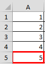
To get the Last Row with data in a Column we need to use the End property of an Excel VBA Range.

Dim lastRow as Range

'Get Last Row with Data in Column
Debug.Print Range("A1").End(xlDown).Row 'Result: 5
Set lastRow = Range("A1").End(xlDown).EntireRow

'Get Last Cell with Data in Row
Dim lastRow as Range
Set lastRow = Range("A1").End(xlDown)

Last Row with Data in Worksheet

To get the Last Row with data in a Worksheet we need to use the SpecialCells or Find properties of an Excel VBA Range.

Dim lastRow as Range, ws As Worksheet
Set ws = ActiveSheet

'Get Last Row with Data in Worksheet using SpecialCells
Debug.Print ws.Cells.SpecialCells(xlCellTypeLastCell).Row
Set lastRow = ws.Cells.SpecialCells(xlCellTypeLastCell).EntireRow 

'Get Last Row with Data in Worksheet using Find
Debug.Print Debug.Print ws.Cells.Find(What:="*", _
        After:=ws.Cells(1), _
        Lookat:=xlPart, _
        LookIn:=xlFormulas, _
        SearchOrder:=xlByRows, _
        SearchDirection:=xlPrevious, _
        MatchCase:=False).Row
Set lastRow = Debug.Print ws.Cells.Find(What:="*", _
        After:=ws.Cells(1), _
        Lookat:=xlPart, _
        LookIn:=xlFormulas, _
        SearchOrder:=xlByRows, _
        SearchDirection:=xlPrevious, _
        MatchCase:=False).EntireRow

Last Row in Worksheet UsedRange

To get the Last Row in the Worksheet UsedRange we need to use the UsedRange property of an VBA Worksheet.

'Get Last Row in Worksheet UsedRange
Dim lastRow as Range, ws As Worksheet
Set ws = ActiveSheet
Debug.Print ws.UsedRange.Rows(ws.UsedRange.Rows.Count).Row
Set lastRow = ws.UsedRange.Rows(ws.UsedRange.Rows.Count).EntireRow

The UsedRange represents a Range used by an Excel Worksheet. The Used Range starts at the first used cell and ends with the most right, down cell that is used by Excel. This last cell does not need to have any values or formulas as long as it was edited or formatted in any point in time

VBA Last Column

The Last Column may as be interpreted as:

Last Column with Data in a Row
Last Column with Data in Worksheet
Last Column in Worksheet UsedRange

Last Column with Data in a Row

Last Column with Data in a Worksheet

To get the Last Column with data in a Worksheet we need to use the SpecialCells or Find properties of an Excel VBA Range.

Dim lastColumn as Range, ws As Worksheet
Set ws = ActiveSheet

'Get Last Column with Data in Worksheet using SpecialCells
Debug.Print ws.Cells.SpecialCells(xlCellTypeLastCell).Column
Set lastColumn = ws.Cells.SpecialCells(xlCellTypeLastCell).EntireColumn 

'Get Last Column with Data in Worksheet using Find
Debug.Print Debug.Print ws.Cells.Find(What:="*", _
        After:=ws.Cells(1), _
        Lookat:=xlPart, _
        LookIn:=xlFormulas, _
        SearchOrder:=xlByRows, _
        SearchDirection:=xlPrevious, _
        MatchCase:=False).Column
Set lastColumn = Debug.Print ws.Cells.Find(What:="*", _
        After:=ws.Cells(1), _
        Lookat:=xlPart, _
        LookIn:=xlFormulas, _
        SearchOrder:=xlByRows, _
        SearchDirection:=xlPrevious, _
        MatchCase:=False).EntireColumn

Last Column in Worksheet UsedRange

To get the Last Column in the Worksheet UsedRange we need to use the UsedRange property of an VBA Worksheet.

'Get Last Column in Worksheet UsedRange
Dim lastColumn as Range, ws As Worksheet
Set ws = ActiveSheet
Debug.Print ws.UsedRange.Columns(ws.UsedRange.Columns.Count).Column
Set lastColumn = ws.UsedRange.Columns(ws.UsedRange.Columns.Count).EntireColumn

VBA Last Cell

The Last Cell may as be interpreted as:

Last Cell in a series of data
Last Cell with Data in Worksheet
Last Cell in Worksheet UsedRange

Last Cell in a series of data

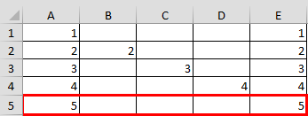
To get the Last Cell in a series of data (table with non-blank values) we need to use the End property of an Excel VBA Range.

Dim lastCell as Range

'Get Last Cell in a series of data
Dim lastCell as Range
Set lastCell = Range("A1").End(xlRight).End(xlDown)
Debug.Print "Row: " & lastCell.row & ", Column: " & lastCell.column

Last Cells with Data in Worksheet

To get the Last Cell with data in a Worksheet we need to use the SpecialCells or Find properties of an Excel VBA Range.

Dim lastCell as Range, ws As Worksheet
Set ws = ActiveSheet

'Get Last Cell with Data in Worksheet using SpecialCells
Set lastCell = ws.Cells.SpecialCells(xlCellTypeLastCell)
Debug.Print "Row: " & lastCell.row & ", Column: " & lastCell.column

'Get Last Cell with Data in Worksheet using Find
Set lastColumn = Debug.Print ws.Cells.Find(What:="*", _
        After:=ws.Cells(1), _
        Lookat:=xlPart, _
        LookIn:=xlFormulas, _
        SearchOrder:=xlByRows, _
        SearchDirection:=xlPrevious, _
        MatchCase:=False)
Debug.Print "Row: " & lastCell.row & ", Column: " & lastCell.column

Last Cell in Worksheet UsedRange

To get the Last Cell in the Worksheet UsedRange we need to use the UsedRange property of an VBA Worksheet.

'Get Last Cell in Worksheet UsedRange
Dim lastCell as Range, ws As Worksheet
Set ws = ActiveSheet

Set lastCell = ws.UsedRange.Cells(ws.UsedRange.Rows.Count,ws.UsedRange.Columns.Count)
Debug.Print "Row: " & lastCell.row & ", Column: " & lastCell.column

VBA UsedRange

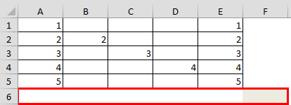
The VBA UsedRange represents the area reserved and saved by Excel as the currently used Range on and Excel Worksheet. The UsedRange constantly expands the moment you modify in any way a cell outside of the previously Used Range of your Worksheet.

The UsedRange is not reduced if you Clear the Contents of Range. The only way to reduce a UsedRange is to delete the unused rows and columns.

How to check the UsedRange

The easiest way to check the currently UsedRange in an Excel Worksheet is to select a cell (best A1) and hitting the following key combination: CTRL+SHIFT+END. The highlighted Range starts at the cell you selected and ends with the last cell in the current UsedRange.

Check UsedRange in VBA

Use the code below to check the area of the UsedRange in VBA:

Dim lastCell As Range, firstCell As Range, ws As Worksheet
Set ws = ActiveSheet
    
Set lastCell = ws.UsedRange.Cells(ws.UsedRange.Rows.Count, ws.UsedRange.Columns.Count)
Set firstCell = ws.UsedRange.Cells(1, 1)
Debug.Print "First Cell in UsedRange. Row: " & firstCell.Row & ", Column: " & firstCell.Column
Debug.Print "Last Cell in UsedRange. Row: " & lastCell.Row & ", Column: " & lastCell.Column

For the screen above the result will be:

First Cell in UsedRange; Row: 2, Column: 2
Last Cell in UsedRange; Row: 5, Column: 6

First UsedCell in UsedRange

The below will return get the first cell of the VBA UsedRange and print its row and column:

Dim firstCell as Range
Set firstCell = ws.UsedRange.Cells(1, 1)
Debug.Print "First Cell in UsedRange. Row: " & firstCell.Row & ", Column: " & firstCell.Column

Last UsedCell in UsedRange

The below will return get the first cell of the VBA UsedRange and print its row and column:

Dim lastCell as Range
Set lastCell = ws.UsedRange.Cells(ws.UsedRange.Rows.Count, ws.UsedRange.Columns.Count)
Debug.Print "Last Cell in UsedRange; Row: " & lastCell.Row & ", Column: " & lastCell.Column

Источник

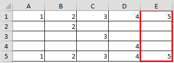
This example illustrates the End property of the Range object in Excel VBA. We will use this property to select the range from the Active Cell to the last entry in a column.

Situation:

Some sales figures in column A. Assume that you will be adding more sales figures over time.

Place a command button on your worksheet and add the following code lines:

1. To select the last entry in a column, simply add the following code line:

Range(«A5»).End(xlDown).Select

Note: instead of Range(«A5»), you can also use Range(«A1»), Range(«A2»), etc. This code line is equivalent to pressing the END+DOWN ARROW.

Result when you click the command button on the sheet:

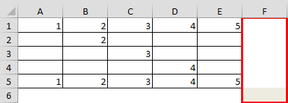
2. To select the range from cell A5 to the last entry in the column, add the following code line:

Range(Range(«A5»), Range(«A5»).End(xlDown)).Select

Result when you click the command button on the sheet:

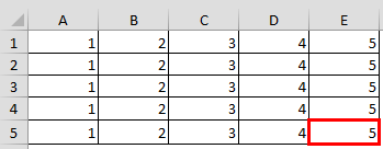
3. To select the range from the Active Cell to the last entry in the column, simply replace Range(«A5») with ActiveCell.

Range(ActiveCell, ActiveCell.End(xlDown)).Select

Result when you select cell A2 and click the command button on the sheet:

Note: you can use the constants xlUp, xlToRight and xlToLeft to move in the other directions. This way you can select a range from the Active Cell to the last entry in a row.

Источник

Синтаксис

Параметры

Примеры

Range End Property Syntax

Moving to the Last Cell

Counting Rows

Creating a Range Array

VBA Coding Made Easy

VBA END Function

How to Use VBA End Function in Excel?

Example #1 – VBA END

Example #2 – VBA END

Example #3 – VBA END

Example #4 – VBA END

Things to Remember

Recommended Articles

End Function in VBA

Table of contents

End Property in VBA

Examples of Excel VBA End Function

Example #1 – Use VBA End Property To Move in Worksheet

Example #2 – Selection Using End Property

Example #3 – Select Right to Left, Right to Bottom, & Top

Recommended Articles

Поиск по меткам

Примеры кода

Скачать

Типовые задачи

Перебор ячеек диапазона (вариант 4)

Работа с текущей областью

Определение границ текущей области

Выделение столбцов / строк текущей области

Сброс форматирования диапазона

Поиск последней строки столбца (вариант 1)

Поиск последней строки столбца (вариант 2)

Поиск «последней» ячейки листа

Разбор клипо-генератора

Читайте также:

Работа с объектом Range

Массивы в VBA

Структуры данных и их эффективность

Автоматическое скрытие/показ столбцов и строк

A Quick Guide to Ranges and Cells

Download the Code

The Webinar

Introduction

Important Notes

The Range Property

The Cells Property of the Worksheet

Using Cells and Range together

The Offset Property of Range

Using the Range CurrentRegion

How to Use

Read Data Rows Only

Remove Header

Using Rows and Columns as Ranges

Using Range in place of Worksheet

Reading Values from one Cell to another

Using the Range.Resize Method

Reading Values to variables

How to Copy and Paste Cells

Reading a Range of Cells to an Array

Going through all the cells in a Range

Formatting Cells

Main Points

What’s Next?

Last Row in a Column

Last Row with Data in Worksheet

Last Row in Worksheet UsedRange

VBA Last Column

Last Column with Data in a Row

Last Column in Worksheet UsedRange

VBA Last Cell

Last Cell in a series of data

Last Cells with Data in Worksheet

Last Cell in Worksheet UsedRange

VBA UsedRange

How to check the UsedRange

Check UsedRange in VBA

First UsedCell in UsedRange