
Поиск значения в таблице (диапазоне, массиве) по значению в первом столбце таблицы с помощью метода VBA Excel WorksheetFunction.VLookup. Синтаксис, параметры, примеры.
WorksheetFunction.VLookup – это метод VBA Excel, который ищет значение в крайнем левом столбце таблицы (диапазона, двумерного массива) и возвращает значение ячейки (элемента массива), находящейся в указанном столбце той же строки. Метод соответствует функции рабочего листа =ВПР (вертикальный просмотр).
Синтаксис
Синтаксис метода WorksheetFunction.VLookup в VBA Excel:
|
WorksheetFunction.VLookup(Arg1, Arg2, Arg3, Arg4) |
Параметры
Описание параметров метода WorksheetFunction.VLookup:
| Параметр | Описание |
|---|---|
| Arg1 (Lookup_value) | Обязательный параметр. Значение, которое необходимо найти в первом столбце таблицы. |
| Arg2 (Table_array) | Обязательный параметр. Таблица с двумя или более столбцами данных. Используется ссылка на диапазон, имя диапазона или массив. |
| Arg3 (Col_index_num) | Обязательный параметр. Номер столбца, значение из которого возвращается. |
| Arg4 (Range_lookup) | Необязательный параметр. Логическое значение, указывающее, должен ли метод VLookup искать точное совпадение или приблизительное. |
Значения параметра Arg4 (Range_lookup), задающие точность сопоставления:
| Значение | Точность сопоставления |
|---|---|
| True | Значение по умолчанию. Метод WorksheetFunction.VLookup находит точное или приблизительное совпадение Arg1 со значением в первом столбце. Если точное совпадение не найдено, используется самое большое значение, меньшее Arg1. Значения в первом столбце таблицы должны быть отсортированы по возрастанию. |
| False | Метод WorksheetFunction.VLookup находит только точное совпадение. Сортировка значений первого столбца таблицы не требуется. Если точное совпадение не найдено, генерируется ошибка. |
Если значение параметра Arg1 является текстом, а Arg4=False, тогда в строке Arg1 можно использовать знаки подстановки (спецсимволы): знак вопроса (?) и звездочку (*). Знак вопроса заменяет один любой символ, а звездочка соответствует любой последовательности символов. Чтобы знак вопроса (?) и звездочка (*) обозначали сами себя, перед ними указывается тильда (~).
Примеры
Примеры обкатывались на следующей таблице:

Поиск значения в таблице
|
Sub Primer1() Dim x x = «Смартфон: « & WorksheetFunction.VLookup(7, Range(«A2:D11»), 2, False) MsgBox x End Sub |
Результат работы кода:

Поиск значения в массиве
|
Sub Primer2() Dim x, y x = Range(«A2:D11») y = «Смартфон: « & WorksheetFunction.VLookup(8, x, 2, False) & vbNewLine _ & «Разрешение экрана: « & WorksheetFunction.VLookup(8, x, 3, False) & vbNewLine _ & «Емкость аккумулятора: « & WorksheetFunction.VLookup(8, x, 4, False) & » мАч» MsgBox y End Sub |
Результат работы кода:

Да, здесь можно немного улучшить структуру кода, применив оператор With...End With:
|
Sub Primer3() Dim x, y x = Range(«A2:D11») With WorksheetFunction y = «Смартфон: « & .VLookup(8, x, 2, False) & vbNewLine _ & «Разрешение экрана: « & .VLookup(8, x, 3, False) & vbNewLine _ & «Емкость аккумулятора: « & .VLookup(8, x, 4, False) & » мАч» End With MsgBox y End Sub |
|
ts-79 Пользователь Сообщений: 246 |
#1 20.01.2014 19:17:04 Добрый день уважаемые! Имеется UserForm с различными элементами. После заполнения данные из UserForm заносятся в соответствующие ячейки последней строки Листа2. Вот кусок кода, где вместо ВПР(FIO.value;Лист3!$B$2:$E$10;3 или 4;0) надо вставить данные из столбцов D и Е Листа3, которые соответствуют значению
Подскажите пожалуйста как это можно сделать, если вообще можно? Изменено: ts-79 — 21.01.2014 13:45:12 |
||
|
The_Prist  Пользователь Сообщений: 14181 Профессиональная разработка приложений для MS Office |
Запишите вставку формулы макросом. А потом замените на значение. Даже самый простой вопрос можно превратить в огромную проблему. Достаточно не уметь формулировать вопросы… |
|
ikki  Пользователь Сообщений: 9709 |
как вариант — вызов WorksheetFunction.Lookup фрилансер Excel, VBA — контакты в профиле |
|
Serge 007 Пользователь Сообщений: 11308 |
#4 20.01.2014 20:52:41
Vlookup <#0> |
||
|
ikki Пользователь Сообщений: 9709 |
точно фрилансер Excel, VBA — контакты в профиле |
|
Бонифаций  Пользователь Сообщений: 120 |
.Cells(LastRow, «C» ).Value = «=VLOOKUP(FIO.value;Лист3!$B$2:$E$10;4;0) « |
|
The_Prist Пользователь Сообщений: 14181 Профессиональная разработка приложений для MS Office |
#7 20.01.2014 22:04:28 Бонифайций, тогда уж по всем правилам надо(.Value не будет вычислять формулу, FIO.value — должно быть экранировано)
Даже самый простой вопрос можно превратить в огромную проблему. Достаточно не уметь формулировать вопросы… |
||
|
ts-79 Пользователь Сообщений: 246 |
#8 21.01.2014 06:50:15
Выдает ошибку #ИМЯ?
Этот вариант думал применить если не получится в одну строчку. |
||||
|
The_Prist Пользователь Сообщений: 14181 Профессиональная разработка приложений для MS Office |
У меня никаких ошибок не выдает. Ошибку #ИМЯ! может выдать как раз в том случае, если Вы воспользовались советом Бонифаций и использовали свойство .Value. Приложите свой пример, в котором эта ошибка появляется. Даже самый простой вопрос можно превратить в огромную проблему. Достаточно не уметь формулировать вопросы… |
|
ts-79 Пользователь Сообщений: 246 |
#10 21.01.2014 13:40:18
Спасибо за помощь. Решение нашел через Find.
На всякий случаю прикладываю файл. Прикрепленные файлы
Изменено: ts-79 — 21.01.2014 13:44:49 |
||||||
In this Article
- VLOOKUP
- Application.WorksheetFunction.VLookup
- Application.VLookup vs Application.WokrsheetFunction.VLookup
- WorksheetFunction.XLOOKUP
This article will demonstrate how to use the VLOOKUP and XLOOKUP functions in VBA.
The VLOOKUP and XLOOKUP functions in Excel are extremely useful. They can also be used in VBA Coding.
VLOOKUP
There are two ways to call the VLOOKUP Function in VBA:
- Application.WorksheetFunction.Vlookup
- Application.Vlookup
The two methods worked identically, except for how they handle errors.
Application.WorksheetFunction.VLookup
This example will demonstrate the first method.
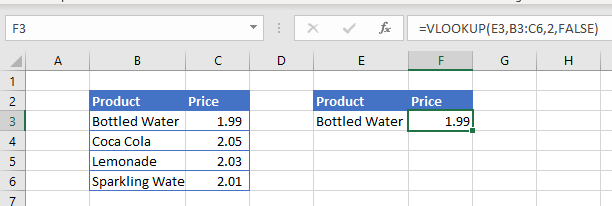
Here we’ve created a VLOOKUP formula in Excel that we will replicate in VBA:
Sub LookupPrice()
   ActiveCell = Application.WorksheetFunction.VLookup(Range("E3"), Range("B2:C6"), 2, False)
End Sub
This will result in the following:
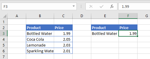
Note that the actual result was written to cell F3 instead of the formula!
If we wish to return a formula to Excel instead of a value, write the VLOOKUP into a formula:
Sub LookupPrice()
   ActiveCell = "=VLOOKUP(E3,B2:C6,2,FALSE)"
End Sub
Or you can write the formula to a cell using R1C1 notation, which creates a formula with relative references that can be used over a range of cells:
Sub LookupPrice()
  ActiveCell = "=VLOOKUP(RC[-1],RC[-4]:R[3]C[-3],2,FALSE)"
End Sub
You can also use variables to define the VLOOKUP inputs:
Sub LookupPrice()
 Dim strProduct As String
 Dim rng As Range
 strProduct = Range("E3")
 Set rng = Range("B2:C6")
 ActiveCell = Application.WorksheetFunction.VLookup(strProduct, rng, 2, False)
End Sub
Of course, instead of writing the results of the function to a cell, you can write the results to a variable:
Sub LookupPrice()
  Dim strProduct As String
  Dim rng As Range
  Dim strResult as String

  strProduct = Range("E3")
  Set rng = Range("B2:C6")
  strResult = Application.WorksheetFunction.VLookup(strProduct, rng, 2, False)
End Sub
Application.VLookup vs Application.WokrsheetFunction.VLookup
In the examples above, we can use either of the methods and they will return the same result. However what if we were looking up a Product that doesn’t exist – what result would this return? Each function would return a very different result.
Normally when using VLOOKUP in Excel, if the Lookup does not find the correct answer, it returns #N/A back to the cell. However, if we use the example above and look for a product that does not exist, we will end up with a VBA Error.
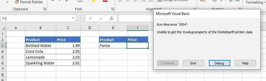
We can trap for this error in our code and return a more user friendly message when the item we are looking for is not found.
Sub LookupPrice()
On Error GoTo eh
ActiveCell = Application.WorksheetFunction.VLookup(Range("E3"), Range("B2:C6"), 2, False)
Exit Sub
eh:
MsgBox "Product not found - please try another product"
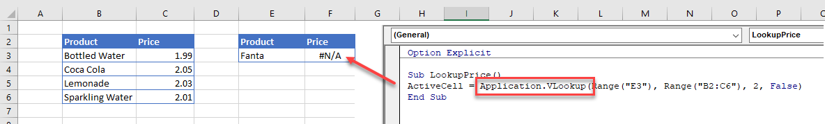
End SubAlternatively, we can amend our VBA code to use Application.Vlookup instead of Application.WorksheetFunction.VLookup.
Sub LookupPrice()
  ActiveCell = Application.VLookup(Range("E3"), Range("B2:C6"), 2, False)
End Sub
When we do this, the #N/A that we have come to expect when a lookup value is not found, is returned to the cell.
WorksheetFunction.XLOOKUP
The XLOOKUP function has been designed to replace the VLOOKUP and HLOOKUP functions in Excel. It is only available to Office 365 so using this function is quite restrictive is some of your users are using older versions of Excel.
It works in much the same ways in VBA as the VLOOKUP function.
Sub LookupPriceV()
   ActiveCell = Application.WorksheetFunction.XLookup(Range("E3"), Range("B2:B6"), Range("C2:C6"))
End Sub
OR
Sub LookupPriceV()
   ActiveCell = Application.XLookup(Range("E3"), Range("B2:B6"), Range("C2:C6"))
End Sub
Once again, if we wish to use variables, we can write the following code
Sub LookupPriceV()
   Dim strProduct As String
   Dim rngProduct As Range
   Dim rngPrice As Range
   strProduct = Range("E3")
   Set rngProduct = Range("B2:B6")
   Set rngPrice = Range("C2:C6")
   ActiveCell = Application.WorksheetFunction.XLookup(strProduct, rngProduct, rngPrice)
End Sub
If we wish to return a formula to Excel instead of a value, we would need to write the formula into Excel with the VBA code.
Sub LookupPrice()
   ActiveCell = "=XLOOKUP(E3,B3:B6,C3:C6)"
End Sub
Or you can write the formula to a cell using R1C1 notation.
Sub LookupPrice()
  ActiveCell.Formula2R1C1 = "=XLOOKUP(RC[-1],RC[-4]:R[3]C[-4],RC[-3]:R[3]C[-3])"
End Sub
One of the major advantages of using XLOOKUP vs VLOOKUP is the ability to lookup a range of columns, and return the value in each column.
Lets look at the following example:
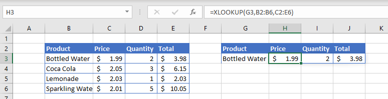
We have created the formula in cell H3 where it is looking up the values in the range C2:E6. Due to the fact that these are multiple columns, it will automatically populate columns I and J with the matching results found. The formula SPILLS over into columns I and J without us having to use CTRL+SHIFT for an array formula – this ability for the formula to SPILL across is one of the new additions for Excel 365.
To replicate this with VBA code, we can type the following in our macro:
Sub LookupPrice()
   ActiveCell.Formula2R1C1 = "=XLOOKUP(RC[-1],RC[-6]:R[3]C[-6],RC[-5]:R[3]C[-3])"
End Sub
Where the formula is using the R1C1 (rows and columns) syntax instead of the A1 (range) syntax. This will result in the formulas being entered into Excel as shown in the graphic above.
You cannot lookup multiple columns if you are using the WorksheetFunction method.
|
vba вместо ВПР |
||||||||
Ответить |
||||||||
Ответить |
||||||||
Ответить |
||||||||
Ответить |
||||||||
Ответить |
||||||||
Ответить |


 WorksheetFunction.VLookup, он же Application.VLookup это та же функция ВПР, тока в другой обертке.
In my earlier post, I had written about VLOOKUP in Excel. It was a massive post of around 2500 words, it explains most of the things about the vertical lookup function in excel. Today’s post is an extension to that post and here we will understand how to apply a VLOOKUP in VBA.
If you haven’t read that post then I would strongly recommend you read that post before going any further. [Read Here]
Assuming that you have basic knowledge of the VLOOKUP function we will move further.
Note: To perform these programs yourself, you may need to enable macros in excel. Read this post to know how to do this.
Syntax of VBA VLOOKUP
You can use VLookUp in macros by following any of the below ways:
Application.VLOOKUP(lookup_value, table_array, column_index, range_lookup)
Or
Application.WorksheetFunction.VLOOKUP(lookup_value, table_array, column_index, range_lookup)
Note: If you are searching for something similar to the VLOOKUP function for Access then probably you should use DLOOKUP.
5 Examples of Using VLOOKUP in VBA
Now let’s move to some practical examples of using VLookUp in VBA codes.
Example 1
Using VLookUp find the monthly salary of “Justin Jones” from the below table. Display the salary using a dialog box.

Below is the code for this:
Sub FINDSAL()
Dim E_name As String
E_name = "Justin Jones"
Sal = Application.WorksheetFunction.VLookup(E_name, Sheet1.Range("B3:D13"), 3, False)
MsgBox "Salary is : $ " & Sal
End Sub

Explanation: In this code, we have used a variable ‘E_name’ to store the employee name whose salary is to be fetched. After this, we have simply supplied the employee name and other required arguments to the VLOOKUP and it returns the salary of the corresponding Employee.
Example 2
Now make the above program a little customizable by accepting the Employee name from the user. If the user enters any Employee name that is not present in the table then the program should be able to convey this clearly to the user.
To accomplish this we can use the below code:
Sub FINDSAL()
On Error GoTo MyErrorHandler:
Dim E_name As String
E_name = InputBox("Enter the Employee Name :")
If Len(E_name) > 0 Then
 Sal = Application.WorksheetFunction.VLookup(E_name, Sheet1.Range("B3:D13"), 3, False)
 MsgBox "Salary is : $ " & Sal
Else
 MsgBox ("You entered an invalid value")
End If
Exit Sub
MyErrorHandler:
If Err.Number = 1004 Then
 MsgBox "Employee Not Present in the table."
End If
End Sub
Explanation: In this code, we are accepting the user input using an InputBox function. If the Employee name entered by the user is found, then VLookUp returns its corresponding salary. However, if the employee name is not present in the table then VLOOKUP throws a “1004 Error”.
And, we have created an error handler to catch such cases for conveying the user that entered employee name doesn’t exist.
Example 3
In this example we will try to write a code that adds the Department field from the Employee Table 1 to our old Employee Table.

As you can see that in both these tables there is only one common column i.e. Employee_ID. So, in this case, we will have to apply the VLookUp based on the Employee ID.
Below is the code to do this:
Sub ADDCLM()
On Error Resume Next
Dim Dept_Row As Long
Dim Dept_Clm As Long
Table1 = Sheet1.Range("A3:A13") ' Employee_ID Column from Employee table
Table2 = Sheet1.Range("H3:I13") ' Range of Employee Table 1
Dept_Row = Sheet1.Range("E3").Row ' Change E3 with the cell from where you need to start populating the Department
Dept_Clm = Sheet1.Range("E3").Column
For Each cl In Table1
 Sheet1.Cells(Dept_Row, Dept_Clm) = Application.WorksheetFunction.VLookup(cl, Table2, 2, False)
 Dept_Row = Dept_Row + 1
Next cl
MsgBox "Done"
End Sub

Explanation: This code takes each ‘lookup_value’ from the Employee ID field (one at a time), looks up its corresponding Department, and then populates the corresponding department value at the appropriate place.
Please note that in this code we have just pasted the result of the VLOOKUP formula, and not the VLookUp formula itself (Refer Example 5).
Example 4
In this example we will try to write a code that displays all the details of an employee from the Employee table (as shown below) when its Employee ID is entered.

Below is the code that can accomplish this:
Sub FETCH_EMP_DETAILS()
On Error GoTo MyErrorHandler:
Dim E_id As Long
E_id = InputBox("Enter the Employee ID :")
Det = "Employee ID : " & Application.WorksheetFunction.VLookup(E_id, Sheet1.Range("A3:E13"), 1, False)
Det = Det & vbNewLine & "Employee Name : " & Application.WorksheetFunction.VLookup(E_id, Sheet1.Range("A3:E13"), 2, False)
Det = Det & vbNewLine & "Employee SSN : " & Application.WorksheetFunction.VLookup(E_id, Sheet1.Range("A3:E13"), 3, False)
Det = Det & vbNewLine & "Monthly Salary : " & Application.WorksheetFunction.VLookup(E_id, Sheet1.Range("A3:E13"), 4, False)
Det = Det & vbNewLine & "Department : " & Application.WorksheetFunction.VLookup(E_id, Sheet1.Range("A3:E13"), 5, False)
MsgBox "Employee Details : " & vbNewLine & Det
Exit Sub
MyErrorHandler:
If Err.Number = 1004 Then
 MsgBox "Employee Not Present in the table."
ElseIf Err.Number = 13 Then
 MsgBox "You have entered an invalid value."
End If
End Sub

Explanation: In this example, we have asked the user to enter the Employee Id and then we have used multiple VLookUp Statements and concatenated their outputs to show all the details in a single message box.
Example 5
Redo example 3 but this time paste the whole VLookUp formula instead of pasting only the result.
Below is the code for doing this:
Sub ADDCLM()
On Error Resume Next
Dim Dept_Row As Long
Dim Dept_Clm As Long
ctr = 0
Table1 = Sheet1.Range("A3:A13") ' Employee_ID Column from Employee table
Table2 = Sheet1.Range("H3:I13") ' Range of Employee Table 1
Dept_Row = Sheet1.Range("E3").Row ' Change E3 with the cell from where you need to start populating the Department
Dept_Clm = Sheet1.Range("E3").Column
For Each cl In Table1
 Sheet1.Cells(Dept_Row, Dept_Clm).FormulaR1C1 = "=VLOOKUP(RC[-4], R3C8:R13C9, 2, False)"
 Dept_Row = Dept_Row + 1
 ctr = ctr + 1
Next cl
MsgBox "Done"
End Sub

Explanation: This code is very similar to the one that we have discussed in Example 3, the only difference between these formulas is that here we are copying the VLookUp formula directly in the cells.
In this code, we have applied the VLOOKUP in R1C1 form. So, the formula =VLOOKUP(RC[-4], R3C8:R13C9, 2, False) means =VLOOKUP(<4 cells to the left of current cell>, <Range of Employee Table 1>, <column to be fetched>, <exact match>).
One thing that is worth noting here is: the square brackets ( [ ] ) in your R1C1 formula indicate that you are specifying a relative range. If you want to specify an absolute range, you need to specify the R1C1 cells without brackets; e.g. R3C8:R13C9.
So, this was all about VBA VLOOKUP .