Excel totals by name - Word и Excel - помощь в работе с программами

Содержание

5 ways to sum a column in Excel
How to sum a column in Excel with one click
How to total columns in Excel with AutoSum
Use the SUM function to total a column
Use Subtotal in Excel to sum only filtered cells
Convert your data into Excel table to get total for your column
Total the data in an Excel table
Set the aggregate function for a Total Row cell
Need more help?
Adding totals by name on separate worksheet
Adding totals by name on separate worksheet
Re: Need help adding totals by name on seperate worksheet
Re: Need help adding totals by name on seperate worksheet
Re: Adding totals by name on seperate worksheet
Re: Adding totals by name on separate worksheet
Re: Adding totals by name on separate worksheet
Re: Adding totals by name on separate worksheet
Re: Adding totals by name on separate worksheet

5 ways to sum a column in Excel

by Alexander Frolov, updated on March 15, 2023

This tutorial shows how to sum a column in Excel 2010 — 2016. Try out 5 different ways to total columns: find the sum of the selected cells on the Status bar, use AutoSum in Excel to sum all or only filtered cells, employ the SUM function or convert your range to Table for easy calculations.

If you store such data as price lists or expense sheets in Excel, you may need a quick way to sum up prices or amounts. Today I’ll show you how to easily total columns in Excel. In this article, you’ll find tips that work for summing up the entire column as well as hints allowing to sum only filtered cells in Excel.

Below you can see 5 different suggestions showing how to sum a column in Excel. You can do this with the help of the Excel SUM and AutoSum options, you can use Subtotal or turn your range of cells into Excel Table which will open new ways of processing your data.

How to sum a column in Excel with one click

There is one really fast option. Just click on the letter of the column with the numbers you want to sum and look at the Excel Status bar to see the total of the selected cells.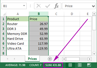

Being really quick, this method neither allows copying nor displays numeric digits.

How to total columns in Excel with AutoSum

If you want to sum up a column in Excel and keep the result in your table, you can employ the AutoSum function. It will automatically add up the numbers and will show the total in the cell you select.

To avoid any additional actions like range selection, click on the first empty cell below the column you need to sum.
Navigate to the Home tab -> Editing group and click on the AutoSum button.
You will see Excel automatically add the =SUM function and pick the range with your numbers.
Just press Enter on your keyboard to see the column totaled in Excel.

This method is fast and lets you automatically get and keep the summing result in your table.

Use the SUM function to total a column

You can also enter the SUM function manually. Why would you need this? To total only some of the cells in a column or to specify an address for a large range instead of selecting it manually.

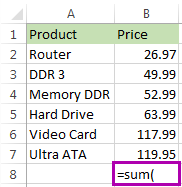
Click on the cell in your table where you want to see the total of the selected cells.
Enter =sum( to this selected cell.
Now select the range with the numbers you want to total and press Enter on your keyboard.

Tip. You can enter the range address manually like =sum(B1:B2000) . It’s helpful if you have large ranges for calculation.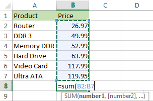

That’s it! You will see the column summed. The total will appear in the correct cell.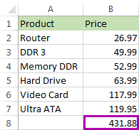

This option is really handy if you have a large column to sum in Excel and don’t want to highlight the range. However, you still need to enter the function manually. In addition, please be prepared that the SUM function will work even with the values from hidden and filtered rows. If you want to sum visible cells only, read on and learn how.

Using the SUM function, you can also automatically total new values in a column as they are added and calculate the cumulative sum.
To multiply one column by another, use the PRODUCT function or multiplication operator. For full details, please see How to multiply two or more columns in Excel.

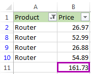
Use Subtotal in Excel to sum only filtered cells

This feature is perfect for totaling only the visible cells. As a rule, these are filtered or hidden cells.

First, filter your table. Click on any cell within your data, go to the Data tab and click on the Filter icon.
You will see arrows appear in the column headers. Click on the arrow next to the correct header to narrow down the data.
Uncheck Select All and tick off only the value(s) to filter by. Click OK to see the results.
Select the range with the numbers to add up and click AutoSum under the Home tab.
Voila! Only the filtered cells in the column are summed up.

If you want to sum visible cells but don’t need the total to be pasted to your table, you can select the range and see the sum of the selected cells on the Excel Status bar. Or you can go ahead and see one more option for summing only filtered cells.

Convert your data into Excel table to get total for your column

If you often need to sum columns, you can convert your spreadsheet to Excel Table. This will simplify totaling columns and rows as well as performing many other operations with your list.

Press Ctrl + T on yourkeyboardto format the range of cells as Excel Table.
You will see the new Design tab appear. Navigate to this tab and tick the checkbox Total Row.
A new row will be added at the end of your table. To make sure you get the sum, select the number in the new row and click on the small down arrow next to it. Pick the Sum option from the list.
Using this option lets you easily display totals for each column. You can see sum as well as many other functions like Average, Min and Max.

This feature adds up only visible (filtered) cells. If you need to calculate all data, feel free to employ instructions from How to total columns in Excel with AutoSum and Enter the SUM function manually to total the column.

Whether you need to sum the entire column in Excel or total only visible cells, in this article I covered all possible solutions. Choose an option that will work for your table: check the sum on the Excel Status bar, use the SUM or SUBTOTAL function, check out the AutoSum functionality or format your data as Table.

If you have any questions or difficulties, don’t hesitate to leave comments. Be happy and excel in Excel!

Источник

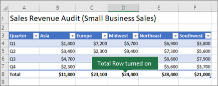
Total the data in an Excel table

You can quickly total data in an Excel table by enabling the Total Row option, and then use one of several functions that are provided in a drop-down list for each table column. The Total Row default selections use the SUBTOTAL function, which allow you to include or ignore hidden table rows, however you can also use other functions.

Click anywhere inside the table.

Go to Table Tools > Design, and select the check box for Total Row.

The Total Row is inserted at the bottom of your table.

Note: If you apply formulas to a total row, then toggle the total row off and on, Excel will remember your formulas. In the previous example we had already applied the SUM function to the total row. When you apply a total row for the first time, the cells will be empty.

Select the column you want to total, then select an option from the drop-down list. In this case, we applied the SUM function to each column:

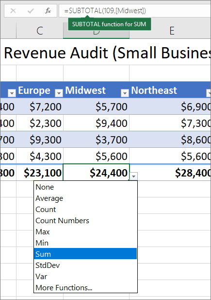
You’ll see that Excel created the following formula: =SUBTOTAL(109,[Midwest]). This is a SUBTOTAL function for SUM, and it is also a Structured Reference formula, which is exclusive to Excel tables. Learn more about Using structured references with Excel tables.

You can also apply a different function to the total value, by selecting the More Functions option, or writing your own.

Note: If you want to copy a total row formula to an adjacent cell in the total row, drag the formula across using the fill handle. This will update the column references accordingly and display the correct value. If you copy and paste a formula in the total row, it will not update the column references as you copy across, and will result in inaccurate values.

Click anywhere inside the table.

Go to Table > Total Row.

The Total Row is inserted at the bottom of your table.

Select the column you want to total, then select an option from the drop-down list. In this case, we applied the SUM function to each column:

You can also apply a different function to the total value, by selecting the More Functions option, or writing your own.

You can quickly total data in an Excel table by enabling the Toggle Total Row option.

Click anywhere inside the table.

Click the Table Design tab > Style Options > Total Row.

The Total row is inserted at the bottom of your table.

Set the aggregate function for a Total Row cell

Note: This is one of several beta features, and currently only available to a portion of Office Insiders at this time. We’ll continue to optimize these features over the next several months. When they’re ready, we’ll release them to all Office Insiders, and Microsoft 365 subscribers.

The Totals Row lets you pick which aggregate function to use for each column.

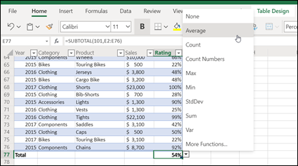
Click the cell in the Totals Row under the column you want to adjust, then click the drop-down that appears next to the cell.

Select an aggregate function to use for the column. Note that you can click More Functions to see additional options.

Need more help?

You can always ask an expert in the Excel Tech Community or get support in the Answers community.

Источник

Adding totals by name on separate worksheet

LinkBack

Thread Tools

Rate This Thread

Display

Adding totals by name on separate worksheet

I have a worksheet where I need to be able to enter a name in one column then a sales amount in the next column and then on a seperate worksheet, show me the sum of all sales by name. I have tried setting up a drop down list where someone can choose from a list of names (there are about 15 possibilities) then enter the sales amount in the next column but don’t know where to go from there to have the totals on a seperate worksheet.

I am somewhat informed on excel but not an expert by any means so go easy on me.

Last edited by mike519; 10-25-2010 at 06:01 PM .

Re: Need help adding totals by name on seperate worksheet

The SUMIF() function will do what you want, and it works easily from separate sheets.

Please edit your title in post #1 and remove the «need help» as that is true of all posts.

If you’ve been given good help, use the icon below to give reputation feedback, it is appreciated.
Always put your code between code tags. [CODE] your code here [/CODE]

?None of us is as good as all of us? — Ray Kroc
?Actually, I *am* a rocket scientist.? — JB (little ones count!)

Re: Need help adding totals by name on seperate worksheet

Pivot tables may be another answer for you.

Re: Adding totals by name on seperate worksheet

Sorry, I looked at the link but have no idea what a Pivot Table is.

Can you elaborate on using sumif?

If, on sheet 1, I have a column where names are selected from a drop down list and then the next column over has a spot where the user enters a sales number, but the user could have multiple entries on the worksheet for the same drop down list name, can you run me through a script that would take all the results from name 1, name 2, name 3, etc and give me a total by name on the next worksheet?

Thanks for your help.

Re: Adding totals by name on separate worksheet

Watch these two videos. You could also upload a sample file that we could do it for you as an example.

Re: Adding totals by name on separate worksheet

Press F1 in Excel read the builtin tutorial on SUMIF(). It should answer all your questions about how it used.

Re: Adding totals by name on separate worksheet

OK, trying Pivot Tables and got the wizard running and had it create a table ona seperate worksheet. Great videos BTW, thanks!

Kinda stuck though as I am not sure where to go from here. I can get the Names showing up in the table as I want but not the totals associated with that particular name. I am attaching the file as suggested for anyone wanting to help a total rookie solve this. I know a little excel but its still more than anyone else I work with does so I have been delegated to doing this but I know I’m a long way from you pros so any help is muchly appreciated.

Re: Adding totals by name on separate worksheet

Glad you liked the videos. Here is your table back with two pivot tables on it. Click on the Pivot Table and see you can make sense of it.

Источник

Possible Duplicate:
Sum Values in One Range Based on Criteria in Another

I have several columns in a spreadsheet with date, item, order etc. but also 2 columns:

Column K — Owed By
Column L — Owed Amount

In column K there will be a couple of different names, say, «Joe» and «Andy», and in column L will be the amount they owe for a particular item.

In another Column, I have Totals for Each Name, and I basically need a formula that will look at Column K see if the name is «Joe» and add the total he owes; then I will change the formula for other names.

Any idea how to go about this?

Источник

I have a spreadsheet with multiple sheets, with lists of names and points assigned to each name. For each individual, I want to sum all their points to determine total points. I’ve given two example sheets in my question, but there could be up to 4 sheets I need to include in the summation. Not all lists are in the same order, and not all names appear in every list. Appearing on each sheet is not a requirement, but I still need a total for all sheets that the individual is present.

example: Sheet 1

    =========== =========== ======== 
    FirstName   LastName     Points  
    =========== =========== ======== 
    Phil        Bloor           7  
    Steve       Burke          14                          
    Teresa      March          18  
    Roger       Sander          9  
    Angela      Umber           3  
    =========== =========== ========

Sheet 2

    =========== =========== ======== 
    FirstName   LastName     Points  
    =========== =========== ======== 
    Phil        Bloor           4  
    Angela      Umber          17                          
    Sarah       McComb         22  
    Roger       Sander          4  
    Shaun       Burns           8  
    =========== =========== ========

Thanks for any help!!!!!

asked Oct 6, 2017 at 17:04

I can’t think of how we can make SUMIF work across sheets conditionally (i.e., based on names present). However, here’s a workaround.

Assuming you already have the First and Last Names listed in your target sheet, you can list the names of all the data sheets alongside the First and Last Name headings. You can then use a combination of SUMIFS and INDIRECT to get the results you want.

Paste this formula in C1:

=SUMIFS(INDIRECT(C$1&"!C:C"),INDIRECT(C$1&"!A:A"),$A2,INDIRECT(C$1&"!B:B"),$B2)

The cells have been frozen so that they can be copied to the other target cells without modifying the formula.

This will fetch you person-wise amounts from each sheet. You can then have a total column at the end in the target sheet, like this:

+---+-----------+----------+--------+--------+-------+
|   |     A     |    B     |   C    |   D    |   E   |
+---+-----------+----------+--------+--------+-------+
| 1 | FirstName | LastName | Sheet1 | Sheet2 | Total |  <-- Headings
+---+-----------+----------+--------+--------+-------+
| 2 | Phil      | Bloor    | 7      | 4      | 11    |
| 3 | Angela    | Umber    | 3      | 17     | 20    |
| 4 | Sarah     | McComb   | 0      | 22     | 22    |
| 5 | Roger     | Sander   | 9      | 4      | 13    |
| 6 | Shaun     | Burns    | 0      | 8      | 8     |
| 7 | Steve     | Burke    | 14     | 0      | 14    |
| 8 | Teresa    | March    | 18     | 0      | 18    |
+---+-----------+----------+--------+--------+-------+

answered Oct 6, 2017 at 17:55

Create tables of each data range in each sheet

Highlight first table and go to Get & Transform (or PowerQuery tab) and click From Table and add the tabl then select Close and load to «Only create a connection».

Repeat for other tables.

Then go to New Query > Combine Queries > Append > Three or more tables > select your tables you just added via queries i.e. Press add until all tables move to right hand side.

Add column tab > custom column > Give new column name as «FullName» and formula as FirstName & LastName > click ok > Transform tab > Group By > FullName.

Then input for New column name = «TotalPoints», Operation = Sum, Column = «Points»

Home tab > Close and load.

You will have a new sheet containing one table created from all the others and which sums the number of points for each combination of FirstName and LastName.

There will be a workbook query called Append1 which you can refresh by clicking the green arrow. This will update the summary table for any new data entered into the tables in the other sheets.

answered Oct 6, 2017 at 18:15

QHarrQHarr

82.9k11 gold badges55 silver badges99 bronze badges

With SUMIFS, SUMPRODUCT, and INDIRECT, you can make this to work with some tweak.

Assuming you have the names listed, here is how you can do if you were to put the formula from cell C2:

=SUMPRODUCT(SUMIFS(INDIRECT("'"&$E$2:$E$3&"'!"&"$C$2:$C$100"),INDIRECT("'"&$E$2:$E$3&"'!"&"$A$2:$A$100"),A2,INDIRECT("'"&$E$2:$E$3&"'!"&"$B$2:$B$100"),B2))

Basically, the INDIRECT with SUMIFS will aggregate all the sheets you need to evaluate and make it to an array with SUMPRODUCT. Hope this helps.

answered Oct 6, 2017 at 18:25

ian0411ian0411

4,0753 gold badges25 silver badges33 bronze badges

Источник

10-25-2010, 12:10 PM

#1

Registered User

Adding totals by name on separate worksheet

Hi all,

I have a worksheet where I need to be able to enter a name in one column then a sales amount in the next column and then on a seperate worksheet, show me the sum of all sales by name. I have tried setting up a drop down list where someone can choose from a list of names (there are about 15 possibilities) then enter the sales amount in the next column but don’t know where to go from there to have the totals on a seperate worksheet.

I am somewhat informed on excel but not an expert by any means so go easy on me.

Thanks!

Mike

Last edited by mike519; 10-25-2010 at 06:01 PM.
10-25-2010, 12:21 PM

#2

Re: Need help adding totals by name on seperate worksheet

The SUMIF() function will do what you want, and it works easily from separate sheets.

Please edit your title in post #1 and remove the «need help» as that is true of all posts.

_________________
Microsoft MVP 2010 — Excel
Visit: Jerry Beaucaire’s Excel Files & Macros

If you’ve been given good help, use the icon below to give reputation feedback, it is appreciated.
Always put your code between code tags. [CODE]

your code here [/CODE]

?None of us is as good as all of us? — Ray Kroc
?Actually, I *am* a rocket scientist.? — JB (little ones count!)
10-25-2010, 12:32 PM

#3

Re: Need help adding totals by name on seperate worksheet
10-25-2010, 06:05 PM

#4

Registered User

Re: Adding totals by name on seperate worksheet

Sorry, I looked at the link but have no idea what a Pivot Table is.

Can you elaborate on using sumif?

If, on sheet 1, I have a column where names are selected from a drop down list and then the next column over has a spot where the user enters a sales number, but the user could have multiple entries on the worksheet for the same drop down list name, can you run me through a script that would take all the results from name 1, name 2, name 3, etc and give me a total by name on the next worksheet?

Thanks for your help.
10-25-2010, 07:00 PM

#5

Re: Adding totals by name on separate worksheet

Hi Mike,

You should look at a few videos like:
http://www.bing.com/videos/watch/vid…KVR5&FORM=LKVR
or
http://www.bing.com/videos/watch/vid…0tables%202003 Which is very close to your question.

Watch these two videos. You could also upload a sample file that we could do it for you as an example.
10-25-2010, 07:03 PM

#6

Re: Adding totals by name on separate worksheet

Press F1 in Excel read the builtin tutorial on SUMIF(). It should answer all your questions about how it used.
10-26-2010, 04:23 PM

#7

Registered User

Re: Adding totals by name on separate worksheet

OK, trying Pivot Tables and got the wizard running and had it create a table ona seperate worksheet. Great videos BTW, thanks!

Kinda stuck though as I am not sure where to go from here. I can get the Names showing up in the table as I want but not the totals associated with that particular name. I am attaching the file as suggested for anyone wanting to help a total rookie solve this. I know a little excel but its still more than anyone else I work with does so I have been delegated to doing this but I know I’m a long way from you pros so any help is muchly appreciated.
10-26-2010, 09:04 PM

#8

Re: Adding totals by name on separate worksheet

Hi Mike,

Glad you liked the videos. Here is your table back with two pivot tables on it. Click on the Pivot Table and see you can make sense of it.

Источник

I’m trying to get a SUM of 4 different columns based on a single name. For instance I’m trying to add «Kit JO Total»+ «PRD JO Total»+ «QC JO Total»+ «PKG JO Total» but only if the Customer is «AMAT». I’m not sure what combination of formulas to use to be able to pull that information and add up all of numbers.

65.3 KB
Views: 6

Change the formulae in G,I,K & M like
=F2#*E2#

Then you can use
=SUM(FILTER(FILTER(G2#:M2#,C2#="AMAT"),ISODD(COLUMN(G:M))))

Change the formulae in G,I,K & M like
=F2#*E2#

Then you can use
=SUM(FILTER(FILTER(G2#:M2#,C2#="AMAT"),ISODD(COLUMN(G:M))))

That is fantastic! Thank you! I’ve never seen the ISODD formula before.

You’re welcome & thanks for the feedback.

Following on Fluff13‘s idea:
=SUM((C2#="AMAT")*(G2#+I2#+K2#+M2#))
or:
=SUM(FILTER(G2#+I2#+K2#+M2#,C2#="AMAT"))

Following on Fluff13‘s idea:
=SUM((C2#=»AMAT»)*(G2#+I2#+K2#+M2#))
or:
=SUM(FILTER(G2#+I2#+K2#+M2#,C2#=»AMAT»))

«=SUM(FILTER(G2#+I2#+K2#+M2#,C2#=»AMAT»))» This is what I was trying to do, but I couldn’t figure out the combination and order to formulate the equation in. The way I was writing it I kept getting a 0 back. Thank you!

You’re welcome & thanks for the feedback.

So I tried the formulas that p45cal suggested to see if those worked, but now I’ve gone back to the formula you gave me and now I’m getting a Value error message. Any idea why? 74485

Have you clicked UNDO too often and undone your changes regarding:

Change the formulae in G,I,K & M like
=F2#*E2#

Have you clicked UNDO too often and undone your changes regarding:

?

That could be it. My formula is «=SUM(FILTER(FILTER(G2#:M2#,C2#="AMAT"),ISODD(COLUMN(G:M))))» it worked earlier and now I’m getting the value error.
The two you suggested didn’t work correctly. The first one came back with 100 hours more for AMAT and 300 hours less for BROAUT, not sure how that happened. The second one came back with a Value error as well.

In the attached is a comparison of all 3 formulae in cells R1:T3; they’re the same.
Since, from your picture, you’re looking to create results for all customers, there’s a pivot table at cell O9 which gives that (there’s a calculated field adding the 4 columns).
Another way is at cell V2.

70.3 KB
Views: 5

Last edited: May 12, 2021

In the attached is a comparison of all 3 formulae in cells R1:T3; they’re the same.
Since, from your picture, you’re lookig to create results for all customers, there’s a pivot table at cell O9 which gives that (there’s a calculated field adding the 4 columns).
Another way is at cell V2.

So I think I figured out what’s happening but I don’t know how to fix it. When I’m typing the formula and I type in G2# it doesn’t collect all the cells in the column it stays in the one specific cell. I don’t know why it’s ignoring the #.

In the attached is a comparison of all 3 formulae in cells R1:T3; they’re the same.
Since, from your picture, you’re lookig to create results for all customers, there’s a pivot table at cell O9 which gives that (there’s a calculated field adding the 4 columns).
Another way is at cell V2.

These work perfect. I don’t understand why they’re not working on my sheet.

I type in G2# it doesn’t collect all the cells

That would suggest that one of the columns is no longer part of a spill range.

I figured it out. I had to put parenthesis around =G2#*E2#. Idk why but it fixed it. Thank you both for your help!

Источник