Excel total of column

Usually, numbers are stored in rows of a single column, so getting the total of those columns is important. However, there are different ways of getting the total. As a beginner, it is important to know the concept of getting the column totals. This article will show you how to get excel totals of columns differently.

Total Column in Excel
- How to Get Column Total in Excel (with Examples)
  - Example #1 – Get Temporary Excel Column Total in Single Click
  - Example #2 – Get Auto Column Total in Excel
  - Example #3 – Get Excel Column Total by Using SUM Function Manually
  - Example #4 – Get Excel Column Total by Using SUBTOTAL Function
- Things to Remember
- Recommended Articles

How to Get Column Total in Excel (with Examples)

Here we will show you how to get total columns in Excel with a few examples.

You can download this Column Total Excel Template here – Column Total Excel Template

Example #1 – Get Temporary Excel Column Total in Single Click

If you need a quick total of the column and see the total of any column, then this option will show a quick sum of numbers in the column.

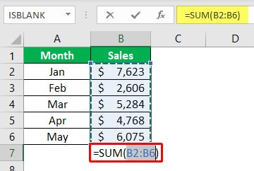
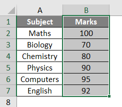
For example, look at the below data in Excel.

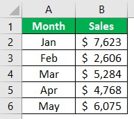
To get the total of this column “B,” select the entire column or the data range from B2 to B6. Then, we need to select the whole column and see the “Status Bar.”

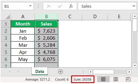
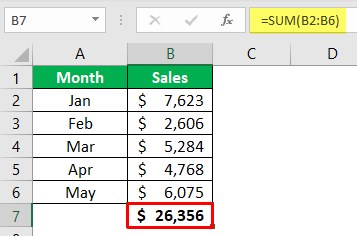
As we can see in the status barAs the name implies, the status bar displays the current status in the bottom right corner of Excel; it is a customizable bar that can be customized to meet the needs of the user.read more, we have a quick sum showing as 26,356.

Instead of selecting the entire column, we must choose the only data range and see the result.

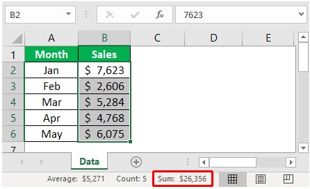
The total is the same, but the only difference is the formatting of numbers. In the previous case, we selected the entire column, and the formatting of numbers was not there. But this time, since we have chosen only the numbers range in the quick sum, too. So then, we can see the same formatting of the selected range.

Example #2 – Get Auto Column Total in Excel

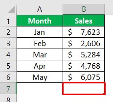
The temporary total can be seen to make the calculations permanently visible in a cell. We can use the autosum option. For example, in the above data, we have data till the 6th row, so in the 7th row, we need the total of the above column numbers.

We must select the cell which is just below the last data cell.

Now press the “ALT + =” shortcut key to insert the AUTOSUM option.

As we can see above, it has automatically inserted the SUM function in excelThe SUM function in excel adds the numerical values in a range of cells. Being categorized under the Math and Trigonometry function, it is entered by typing “=SUM” followed by the values to be summed. The values supplied to the function can be numbers, cell references or ranges.read more upon pressing the shortcut key “ALT + =” and pressing the “Enter” key to get the column total.

Since we have selected only the data range, it has given us the same formatting of the selected cells.

However, there are certain limitations to this AUTOSUM function, especially when we work with a large number of cells. Now, look at the below data.

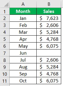
In the above data, we have data range till the 11th row. So in the 12th row, we need the column total, so select cell B12.

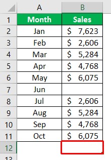
After that, we need to press the ALT + = sign shortcut key to insert the quick SUM function.

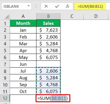
Look at the limitation of the AUTOSUM function. It has selected only four cells above. After the 4th cell, we have a blank cell, so the AUTOSUM shortcut thinks this will be the end of the data and returns only four cells summation.

In this case, this is a small sample size, but when the data is larger, it may go unnoticed. That is where we need to use the manual SUM function.

Example #3 – Get Excel Column Total by Using SUM Function Manually

We can open the SUM function in any cell other than the column of numbers.

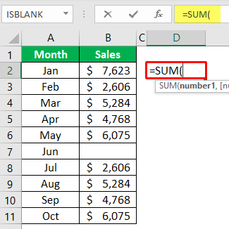
For the SUM function, choose the entire column of “B.”

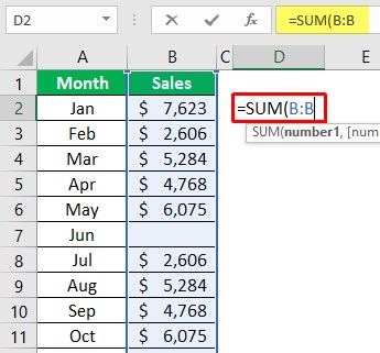
Then, close the bracket and press the “Enter” key to get the result.

So this will take the entire column into consideration and display results accordingly. Since the whole column has been selected, we need not worry about the missing cells.

Example #4 – Get Excel Column Total by Using SUBTOTAL Function

The SUBTOTAL function in excelThe SUBTOTAL excel function performs different arithmetic operations like average, product, sum, standard deviation, variance etc., on a defined range.read more is very powerful to show only displayed cell results.

We must open the SUBTOTAL function first.

Upon opening the SUBTOTAL function, we have many kinds of calculation types. From the list, choose the 9-SUM function.

Next, choose the above range of cells.

Then, close the bracket and press the “Enter key” to get the result.

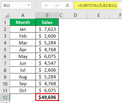
We have got the total of the column. But the question is, if the SUM function returned the same, then what is the point of using SUBTOTAL.

The special thing is that SUBTOTAL displays the calculation only for visible cells. So, for example, apply a filter and choose only any of the three months.

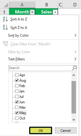
We have chosen only the “Aug, Jun, and May” months. Then, click on “OK” and see the result.

The result of a SUBTOTAL function is limited to only visible cells, not the entire range of cells, so this is the specialty of the SUBTOTAL function.

Things to Remember

The AUTOSUM takes the only reference of non-empty cells, and at the finding of empty cells, it will stop its reference.
If any minus value is between, all those values will be deducted, and the result is the same as the mathematical rule.

SUM function

The SUM function adds values. You can add individual values, cell references or ranges or a mix of all three.

For example:

=SUM(A2:A10) Adds the values in cells A2:10.
=SUM(A2:A10, C2:C10) Adds the values in cells A2:10, as well as cells C2:C10.

SUM(number1,[number2],…)

Argument name	Description
number1 Required	The first number you want to add. The number can be like 4, a cell reference like B6, or a cell range like B2:B8.
number2-255 Optional	This is the second number you want to add. You can specify up to 255 numbers in this way.

Argument name

Description

number1

Required

The first number you want to add. The number can be like 4, a cell reference like B6, or a cell range like B2:B8.

number2-255

Optional

This is the second number you want to add. You can specify up to 255 numbers in this way.

This section will discuss some best practices for working with the SUM function. Much of this can be applied to working with other functions as well.

The =1+2 or =A+B Method – While you can enter =1+2+3 or =A1+B1+C2 and get fully accurate results, these methods are error prone for several reasons:

Typos – Imagine trying to enter more and/or much larger values like this:
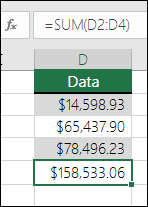
- =14598.93+65437.90+78496.23
Then try to validate that your entries are correct. It’s much easier to put these values in individual cells and use a SUM formula. In addition, you can format the values when they’re in cells, making them much more readable then when they’re in a formula.
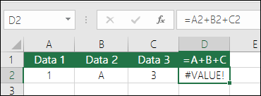
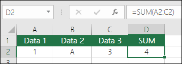
#VALUE! errors from referencing text instead of numbers

If you use a formula like:
- =A1+B1+C1 or =A1+A2+A3
Your formula can break if there are any non-numeric (text) values in the referenced cells, which will return a #VALUE! error. SUM will ignore text values and give you the sum of just the numeric values.
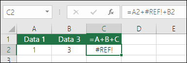
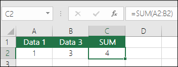
#REF! error from deleting rows or columns

If you delete a row or column, the formula will not update to exclude the deleted row and it will return a #REF! error, where a SUM function will automatically update.
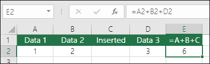
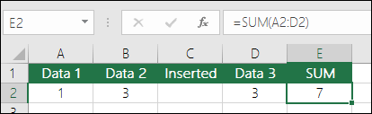
Formulas won’t update references when inserting rows or columns

If you insert a row or column, the formula will not update to include the added row, where a SUM function will automatically update (as long as you’re not outside of the range referenced in the formula). This is especially important if you expect your formula to update and it doesn’t, as it will leave you with incomplete results that you might not catch.
SUM with individual Cell References vs. Ranges

Using a formula like:
- =SUM(A1,A2,A3,B1,B2,B3)
Is equally error prone when inserting or deleting rows within the referenced range for the same reasons. It’s much better to use individual ranges, like:
- =SUM(A1:A3,B1:B3)
Which will update when adding or deleting rows.

I just want to Add/Subtract/Multiply/Divide numbers See this video series on Basic Math in Excel, or Use Excel as your calculator.
How do I show more/less decimal places? You can change your number format. Select the cell or range in question and use Ctrl+1 to bring up the Format Cells Dialog, then click the Number tab and select the format you want, making sure to indicate the number of decimal places you want.
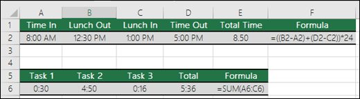
How do I add or subtract Times? You can add and subtract times in a few different ways. For example, to get the difference between 8:00 AM — 12:00 PM for payroll purposes you would use: =(«12:00 PM»-«8:00 AM»)*24, taking the end time minus the start time. Note that Excel calculates times as a fraction of a day, so you need to multiply by 24 to get the total hours. In the first example we’re using =((B2-A2)+(D2-C2))*24 to get the sum of hours from start to finish, less a lunch break (8.50 hours total).

If you’re simply adding hours and minutes and want to display that way, then you can sum and don’t need to multiply by 24, so in the second example we’re using =SUM(A6:C6) since we just need the total number of hours and minutes for assigned tasks (5:36, or 5 hours, 36 minutes).

For more information, see: Add or subtract time.
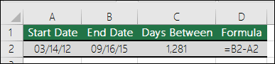
How do I get the difference between dates? As with times, you can add and subtract dates. Here’s a very common example of counting the number of days between two dates. It’s as simple as =B2-A2. The key to working with both Dates and Times is that you start with the End Date/Time and subtract the Start Date/Time.

For more ways to work with dates see: Calculate the difference between two dates.
How do I sum just visible cells? Sometimes, when you manually hide rows or use AutoFilter to display only certain data you also only want to sum the visible cells. You can use the SUBTOTAL function. If you’re using a total row in an Excel table, any function you select from the Total drop-down will automatically be entered as a subtotal. See more about how to Total the data in an Excel table.

Need more help?

You can always ask an expert in the Excel Tech Community or get support in the Answers community.

Definition of Excel Column Total

In excel there are various methods to know the total of numbers inside a column, in this article we will discuss those methods and shortcuts that how do we identify the total sum of numbers in a column. First, we should understand what is the basic definition of Excel Column Total we are talking about. Column Total means the sum of the numbers present inside a column. Now let us go through with various examples on how we can get Totals of Columns in Excel.

Examples of Excel Column Total

Let us discuss examples of Excel Column Total.

You can download this Column Total Excel Template here – Column Total Excel Template

Example #1

Let us begin with the most basic method to know the total of numbers in a column. In this method, we will select a column to see what is the total of the column.

1. Let us make a table of data in sheet 1 as shown below:

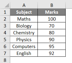
2. Now select whole column B as shown in the image below:

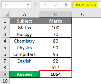
3. In bottom right corner we can see on the status bar that excel automatically calculates the total of the column for us. Refer below screenshot for the preview,

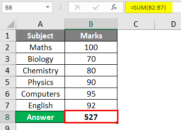
This status bar excel shows us what is the total of column B as Sum which is 527.

Example #2

For example one we have seen how excel has given us total by selecting the total column. But what will happen if we select only the data range in the column rather than the entire column. Let us find out in this example,

1. Let us use the same data from sheet 1 for this example too.

2. Instead of selecting the entire column as we did in example 1, we will select only the data range as shown in below image:

3. Now in the same status bar in the bottom right corner let us check the total as result, it will be same as we have seen in example 1,

So even we select the data range in the column or we select the entire column we will get the same total as result.

Note: Now there is a catch for both example 1 and example 2 that these totals in the columns are temporary means the total can change as soon as the data will change, in the column for example till B7 we had data in the column and if we increase data in B8 the total will increase.

Example #3

In the above examples, we have seen that how excel calculates temporary total in the status bar, however, there are some inbuilt formulas through which a user can calculate the total of the columns in excel by himself, one of such formulas is known as Auto Sum function. It is an inbuilt function in excel which calculates the sum of the numbers of the given data range. There is a keyboard shortcut to use the Auto Sum function in excel which is ‘ALT” + “=” buttons.

1. Now let us copy the same data from sheet 1 to sheet 2 for our data table as shown below:

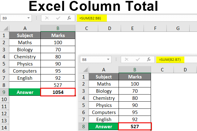
2. In B8 cell let us press the keyboard shortcut we talked about above and see the result as follows:

3. Excel will automatically compute the sum from the data range in the given column, when we press Enter we will get the result as follows:

Example #4

Apart from Auto Sum in Excel which is initiated by a keyboard shortcut, there is an inbuilt sum function in excel which allows us to select specific cells in any columns in excel to compute sum in the columns. Let us use the sum function in this example.

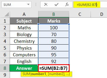
1. In the same data table in cell B9 enter the following formula as shown below:

2. Press “Tab” button from keyboard for the sum function and select the data range from the table as shown in the below image:

3. When we press Enter we will see the result of the sum of the numbers from B2 to B8, remember that in cell B8 we already have the sum of the numbers from B2 to B7.

Explanation of Excel Column Total

In any worksheet of excel data is present in both rows and columns in form of cells. Each individual cells contain data, when these cells contain numbers excel automatically gives us certain features to calculate the total of these numbers by different methods. Some of the methods are inbuilt which is a feature of excel but they give us temporary result, while the formulas which are used to calculate the total of the numbers give us permanent results.

How to Use Excel Column Total?

As we have discussed in the above examples we have seen that there are four methods to calculate Excel Column Total and they are as follows:

First is by selecting the entire column.
The second method is by selecting the data range in the column.
In the third method, we had used the Auto sum function to calculate the total.
The best procedure to calculate the total is by using the sum function.

Things to Remember

There are few things to remember about Excel Column Total and they are as follows,

Column Total Means the sum of numbers in a given column.
When we select a column for column total it ignores the header and calculates the sum of the numbers in a given column.
Auto Sum function only calculates the sum from the data range above the function.
By using Sum function we can select certain cells for which we want the total in the column.

Считаем сумму в столбце в Экселе

Посчитать сумму тех или иных значений в столбцах электронной таблицы Excel можно как вручную, так и автоматически, воспользовавшись базовым инструментарием программы. Кроме того, имеется возможность обычного просмотра итогового значения без его записи в ячейку. Как раз с последнего, наиболее простого мы и начнем.

Способ 1: Просмотр общей суммы

Если вам нужно просто увидеть общее значение по столбцу, в ячейках которого содержаться определенные сведения, при этом постоянно держать эту сумму перед глазами и создавать для ее вычисления формулу не требуется, выполните следующее:

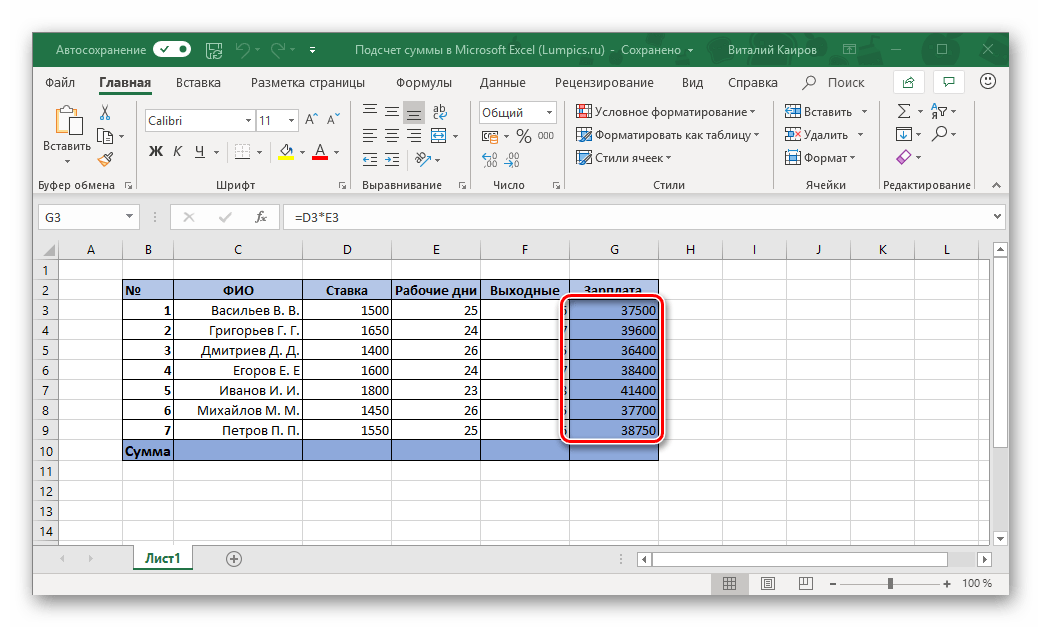
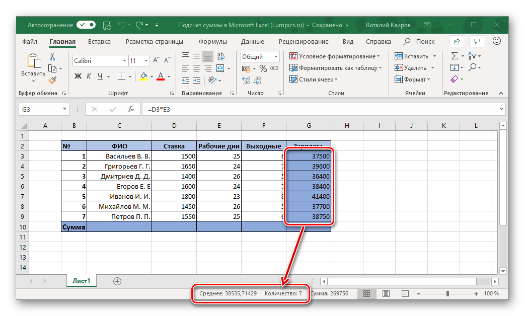
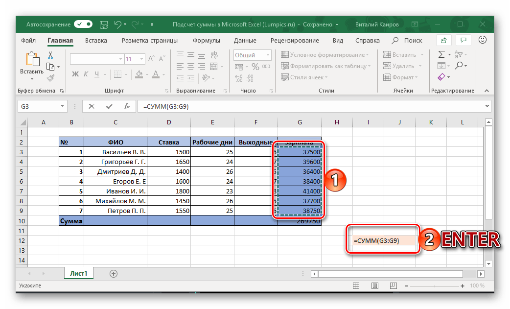
С помощью мышки выделите диапазон ячеек в столбце, сумму значений в котором требуется посчитать. В нашем примере это будут ячейки с 3 по 9 столбца G.

Взгляните на строку состояния (нижняя панель программы) – там будет указана искомая сумма. Отображаться это значение будет исключительно до тех пор, пока выделен диапазон ячеек.

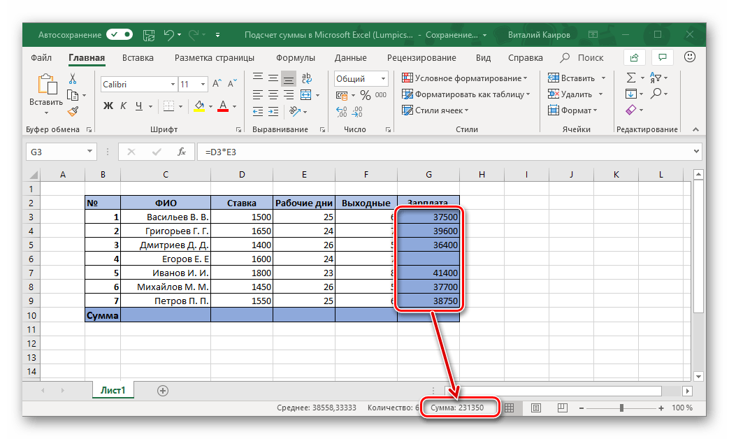
Дополнительно. Такое суммирование работает, даже если в столбце есть пустые ячейки.

Более того, аналогичным образом можно посчитать сумму всех значений в ячейках сразу из нескольких столбцов – достаточно просто выделить необходимый диапазон и посмотреть на строку состояния. Подробнее о том, как это работает, расскажем в третьем способе данной статьи, но уже на примере шаблонной формулы.

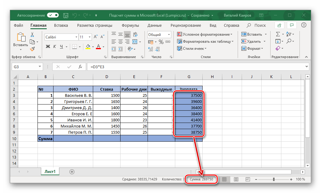
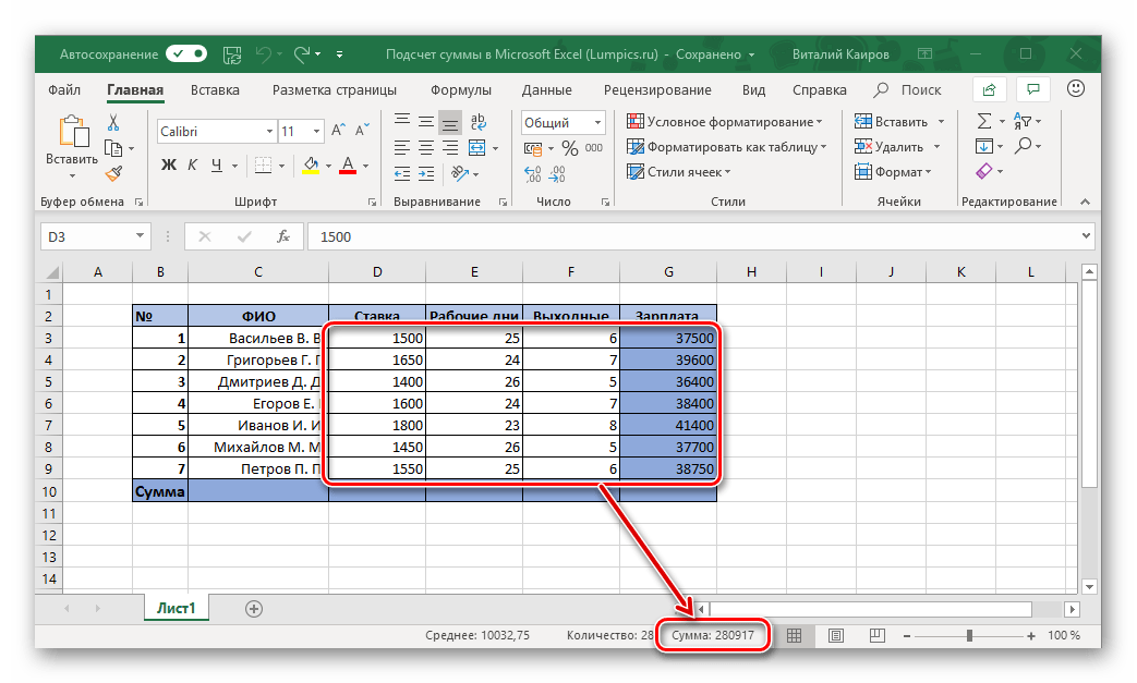
Примечание: Слева от суммы указано количество выделенных ячеек, а также среднее значение для всех указанных в них чисел.

Способ 2: Автосумма

Очевидно, что значительно чаще сумму значений в столбце требуется держать перед глазами, видеть ее в отдельной ячейке и, конечно же, отслеживать изменения, если таковые вносятся в таблицу. Оптимальным решением в таком случае будет автоматическое суммирование, выполняемое с помощью простой формулы.

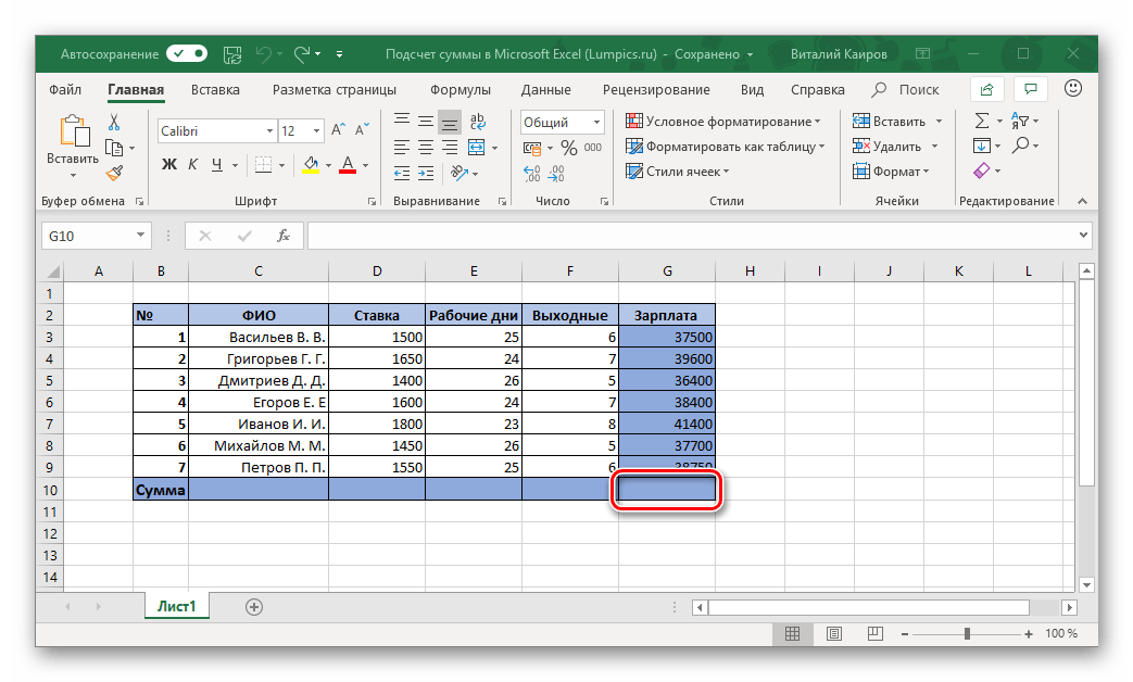
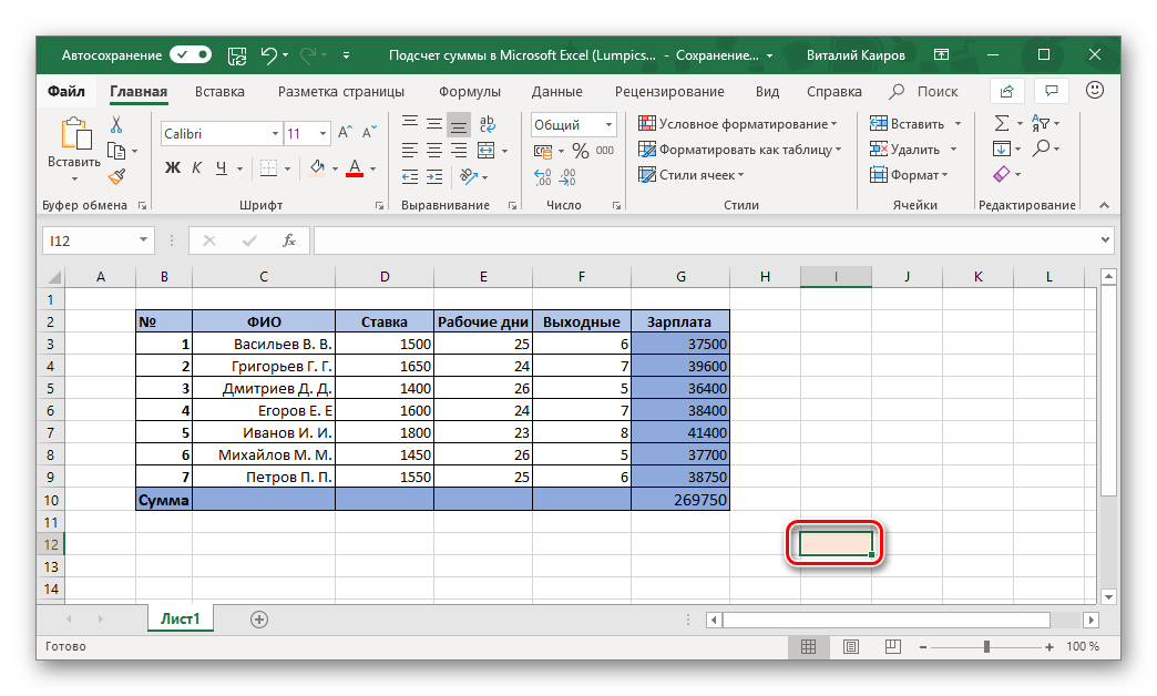
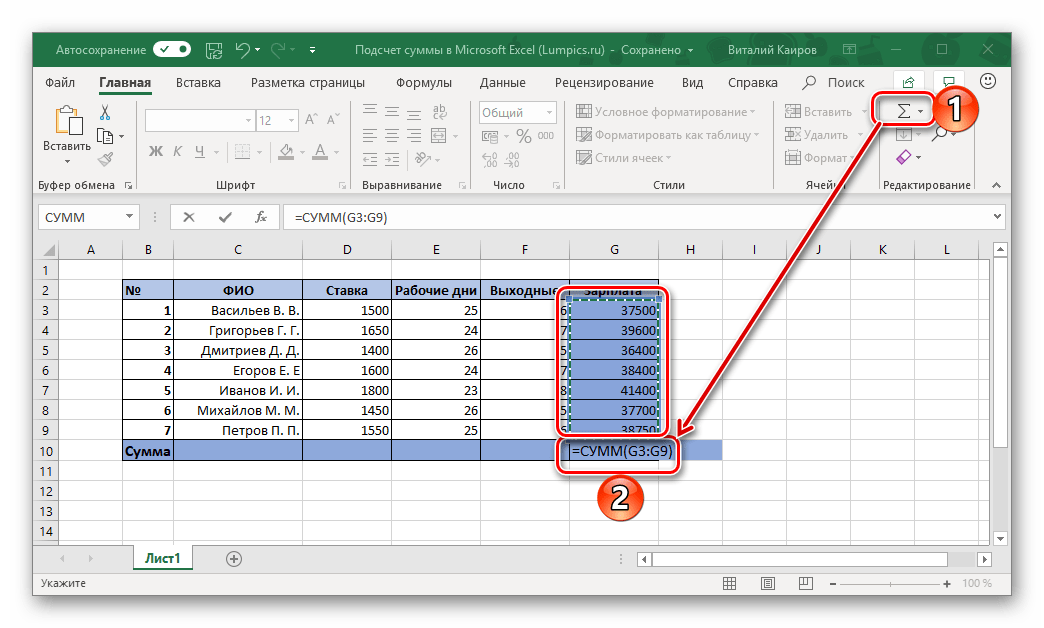
Нажмите левой кнопкой мышки (ЛКМ) по пустой ячейке, расположенной под теми, сумму которых требуется посчитать.

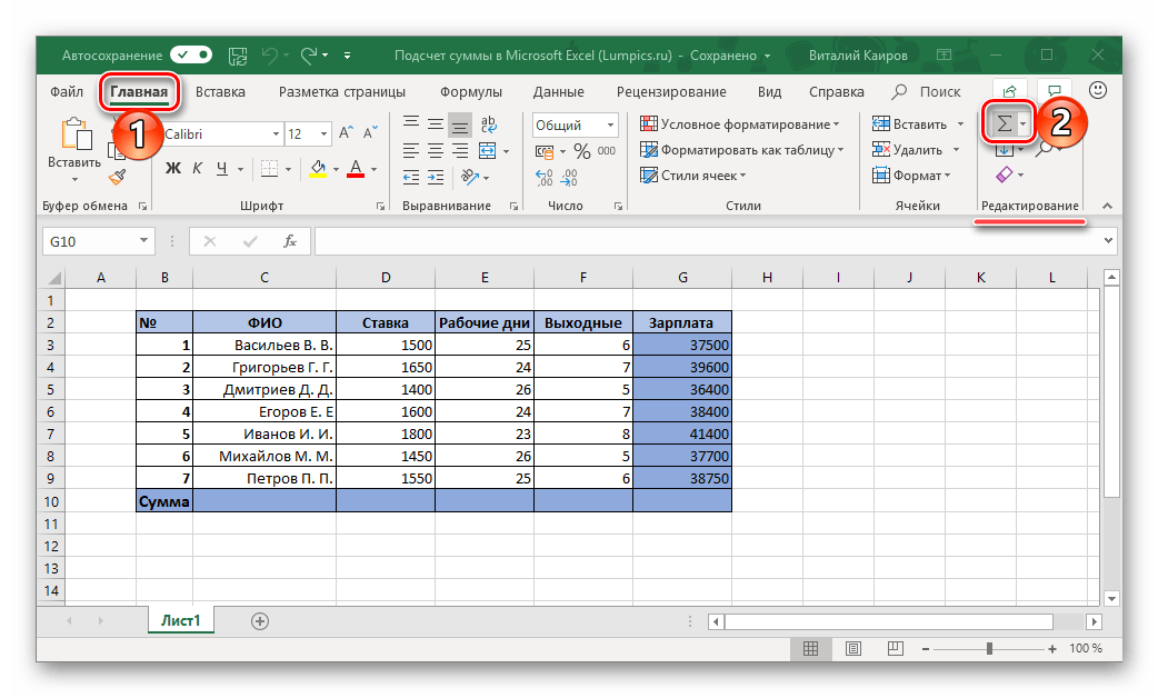
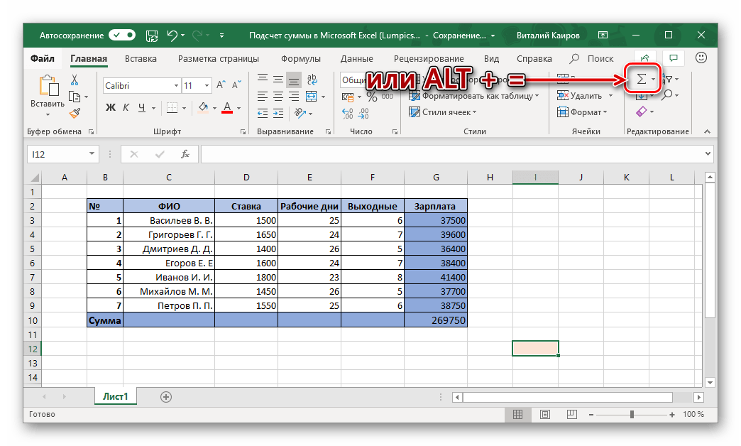
Кликните ЛКМ по кнопке «Сумма», расположенной в блоке инструментов «Редактирование» (вкладка «Главная»). Вместо этого можно воспользоваться комбинацией клавиш «ALT» + «=».

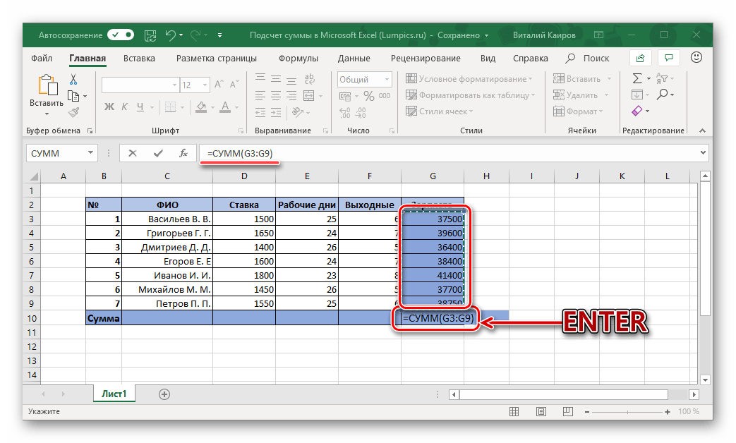
Убедитесь, что в формуле, которая появилась в выделенной ячейке и строке формул, указан адрес первой и последней из тех, которые необходимо суммировать, и нажмите «ENTER».

Вы сразу же увидите сумму чисел во всем выделенном диапазоне.

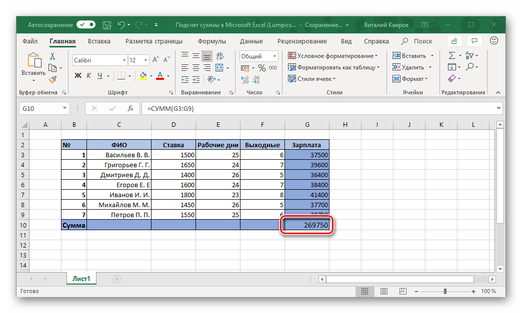
Примечание: Любое изменение в ячейках из выделенного диапазона моментально будет отражаться на итоговой формуле, то есть результат в ней тоже будет меняться.

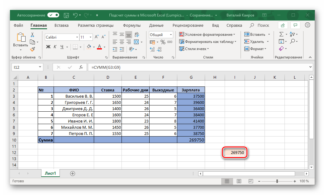
Бывает так, что сумму нужно вывести не в ту ячейку, которая находится под суммируемыми, а в какую-нибудь другую, возможно, расположенную совсем в другом столбце таблицы. В таком случае действовать необходимо следующим образом:

Выделите кликом ячейку, в которой будет вычисляться сумма значений.

Нажмите по кнопке «Сумма» или воспользуйтесь горячим клавишам, предназначенным для ввода этой же формулы.

С помощью мышки выделите диапазон ячеек, которые требуется просуммировать, и нажмите «ENTER».

Совет: Выделить диапазон ячеек можно и немного иным способом – кликните ЛКМ по первой из них, затем зажмите клавишу «SHIFT» и кликните по последней.

Практически точно так же можно суммировать значения сразу из нескольких столбцов или отдельных ячеек, даже если в диапазоне будут пустые ячейки, но обо всем этом далее.

Способ 3: Автосумма нескольких столбцов

Бывает так, что требуется посчитать сумму не в одном, а сразу в нескольких столбцах электронной таблицы Эксель. Делается это практически так же, как и в предыдущем способе, но с одним небольшим нюансом.

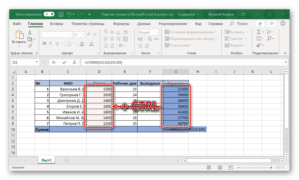
Щелкните ЛКМ по той ячейке, в которую планируете выводить сумму всех значений.

Нажмите по кнопке «Сумма» на панели инструментов или воспользуйтесь предназначенной для ввода этой формулы комбинацией клавиш.

Первый столбец (над формулой) уже будет выделен. Поэтому зажмите клавишу «CTRL» на клавиатуре и выделите следующий диапазон ячеек, который тоже должен входить в рассчитываемую сумму.

Примечание: Если столбцы, которые требуется посчитать, идут подряд, выделять их можно все вместе.

Далее, аналогичным образом, если это еще потребуется, зажимая клавишу «CTRL», выделите ячейки из других столбцов, содержимое которых тоже должно входить в итоговую сумму.

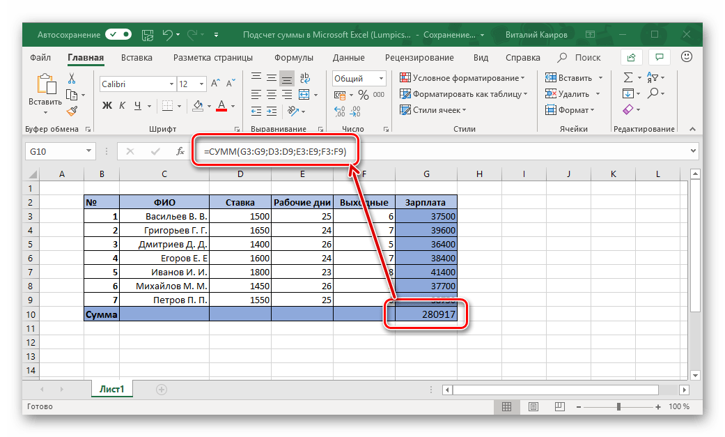
Нажмите «ENTER» для подсчета, после чего в предназначенной для формулы ячейке и строке на панели инструментов появится итоговое вычисление.

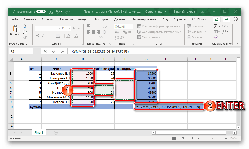
Несложно догадаться, что аналогичным образом можно посчитать сумму значений в отдельных ячейках, состоящих как в разных столбцах, так и в пределах одного.

Для этого нужно просто выделить кликом ячейку для формулы, нажать по кнопке «Сумма» или на горячие клавиши, выделить первый диапазон ячеек, а затем, зажимая клавишу «CTRL», выделить все остальные «участки» таблицы. Сделав это, просто нажмите «ENTER» для отображения результата.

Как и в предыдущем способе, формула суммы может быть записана в любую из свободных ячеек таблицы, а не только в ту, которая находится под суммируемыми.

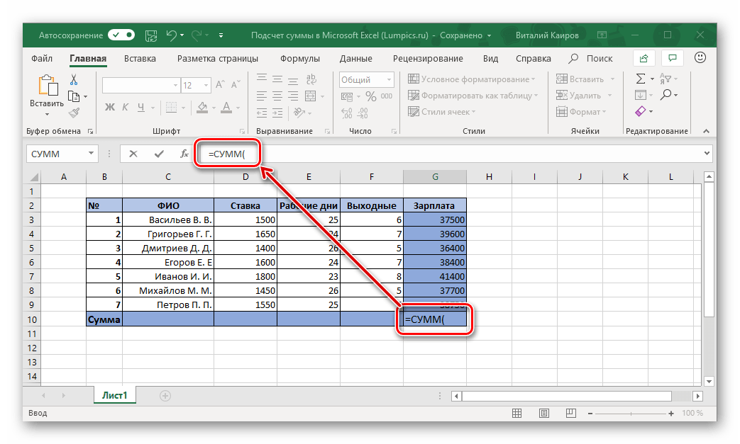
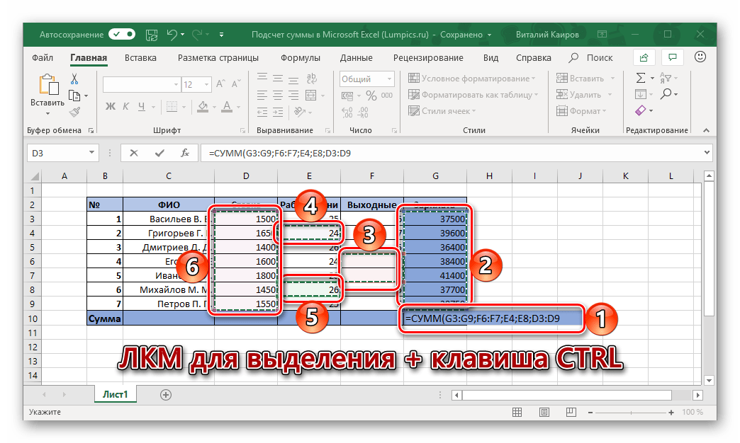
Способ 4: Суммирование вручную

Как и любая формула в Microsoft Excel, «Сумма» имеет свой синтаксис, а потому она может быть прописана вручную. Зачем это нужно? Хотя бы за тем, что таким образом вы точно сможете избежать случайных ошибок при выделении суммируемого диапазона и указании входящих в него ячеек. Более того, даже если вы ошибетесь на каком-то из шагов, исправить это будет так же просто, как банальную опечатку в тексте, а значит, не потребуется проделывать всю работу с нуля, как это иногда приходится делать.

Помимо прочего, самостоятельный ввод формулы позволяет разместить ее не только в любом месте таблицы, но и на любом из листов конкретного электронного документа. Стоит ли говорить о том, что таким образом можно просуммировать не только столбцы и/или их диапазоны, но и просто отдельные ячейки или группы таковых, исключая при этом те, которые не должны быть учтены?

Формула суммы имеет следующий синтаксис:

=СУММ(суммируемые ячейки или диапазон таковых)

То есть все то, что должно быть суммировано, записывается в скобки. Значения, указываемые внутри скобок, должны выглядеть следующим образом:

А теперь перейдем непосредственно к ручному суммированию значений в столбце/столбцах электронной таблицы Эксель.

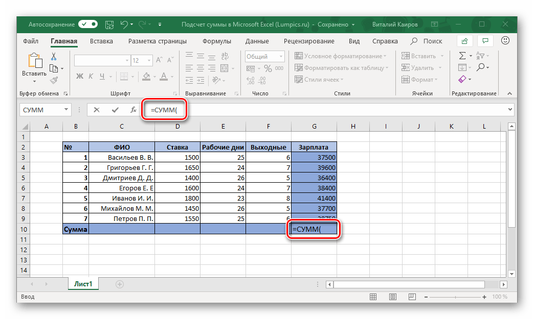
Выделите нажатием ЛКМ ту ячейку, которая будет содержать итоговую формулу.

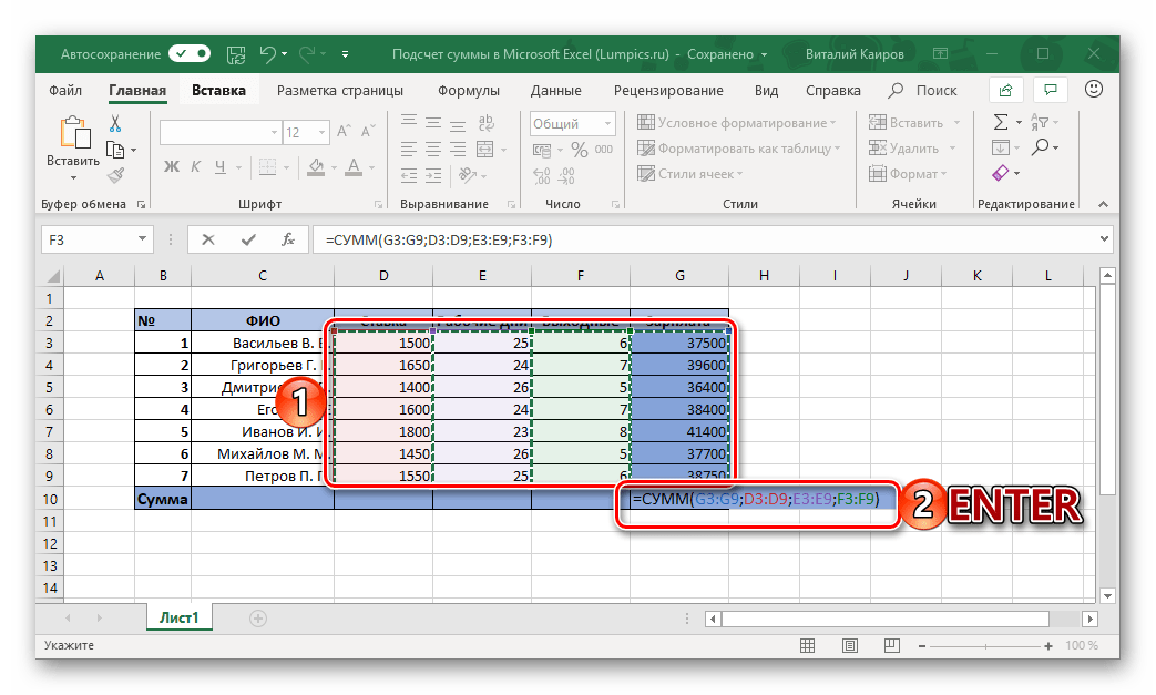
Введите в нее следующее:
=СУММ(

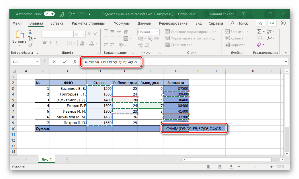
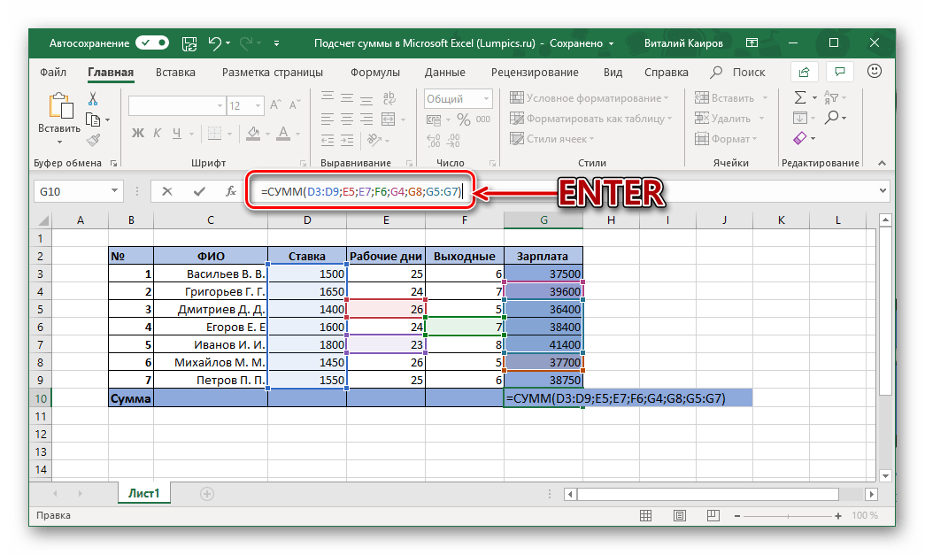
после чего начните поочередно вводить в строке формул адреса суммируемых диапазонов и/или отдельных ячеек, не забывая о разделителях («:» — для диапазона, «;» — для единичных ячеек, вводить без кавычек), то есть делайте все по тому алгоритму, суть которого мы выше подробно описали.

Указав все те элементы, которые требуется просуммировать и убедившись, что вы ничего не пропустили (можно сориентироваться не только по адресам в строке формул, но и по подсветке выделенных ячеек), закройте скобку и нажмите «ENTER» для подсчета.

Примечание: Если вы заметили ошибку в итоговой формуле (например, туда вошла лишняя ячейка или какая-то была пропущена), просто вручную введите правильное обозначение (или удалите лишнее) в строке формул. Аналогичным образом, если и когда это потребуется, можно поступить и с символами-разделителями в виде «;» и «:».

Как вы, наверное, уже могли догадаться, вместо ручного ввода адресов ячеек и их диапазонов можно просто выделять необходимые элементы с помощью мышки. Главное, не забывать при этом удерживать клавишу «CTRL», когда вы переходите от выделения одного элемента к другому.

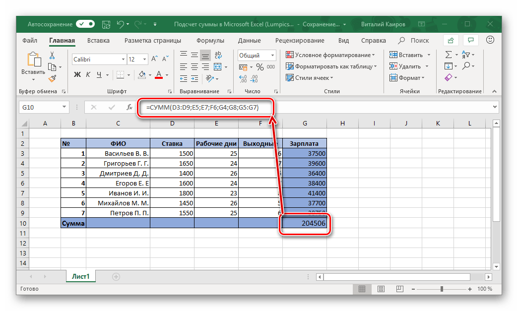
Самостоятельный, ручной подсчет суммы в столбце/столбцах и/или отдельных ячейках таблицы – задача не самая удобная и быстрая в реализации. Но, как мы уже сказали выше, такой подход предоставляет куда более широкие возможности для взаимодействия со значениями и позволяет моментально исправлять случайные ошибки. А вот то, делать ли это полностью вручную, вводя с клавиатуры в формулу каждую переменную, или использовать для этого мышку и горячие клавиши – решать только вам.

Заключение

Даже такая, казалось бы, простая задача, как подсчет суммы в столбце, решается в табличном процессоре Microsoft Excel сразу несколькими способами, и каждый из них найдет свое применение в той или иной ситуации.

Источник

Hundreds of thousands of entries recorded one below the other – a typical description of a massive spreadsheet constructed in MS Excel. Spreadsheets like these would take a lot of time to go through & one would be in dire need of something that could summarize the entries in a particular column. Let’s consider a tabulation of Sales data, for instance, the first thing that might pop in anyone’s mind while looking at it would be, how much has been sold in total?

In this article, we would be covering the different ways of totalling the entries of a column in the below dataset.

Sample Table for Column Totalling

SUM using Cell Range
SUM using Column Name

Method 1 – SUM using Cell Range:

The name of the formula itself is self-explanatory for the functionality that it provides. So, having that sorted out, we shall now look into how to put that into use by trying to total the entries under the Qty. column.

Also read: How to Add in Excel? [Easy Guide]

We shall get things started by clicking on the first blank cell at the bottom of the column as shown below & type =SUM( within.

Typing SUM Formula

Once done, click on the very first entry on the column which would be cell T2 & select all the entries to the very bottom, till T7 as shown in the below image.

Selecting the Range to Total

Include a closing bracket ‘ ) ’, hit ENTER & the total of all the entries shall be displayed in that cell.

Total Displayed!

Method 2 – SUM using Column Name:

There always lies a potential window of error when one has to choose the range of cells to be totaled while constructing a formula. Also, when the workbook is made accessible to a number of users, there is no guarantee that the range given in the formula remains the same. Nevertheless, there is a way around to counter these shortcomings.

Behold!

The COLUMN NAMING!

What this does is help us put a name of our choice over a selected range of cells so that whenever we want to use a particular range of cells in a formula, we might not select the entire set of cells manually but just type in the name which we gave to them!

The execution too would be fairly simple as would be stated below.

We shall get started by selecting the range of cells which we want to total, the column Total Price for instance.

Selecting a Range to Name

Once done, click on the cell address box as shown below & type the name of your choice.

Naming the Selected Range

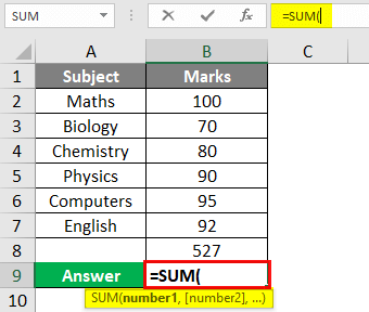
Now we trace resume to the very first step of the previous method in which we type the formula, =SUM( within the first blank cell at the bottom of the column as shown below.

Including SUM below Total Price column

Here’s the cool part, where we need to type in the name we gave rather than selecting the cells. Type a few letters of the name & Excel shall suggest the name available for selection as shown in the below image.

Name of the Range gets Suggested!

Click on the named range & include a closing bracket ‘ ) ‘ to complete the formula. Hit ENTER & the total calculated shall be displayed within cell V8.

Including Named Range within SUM

Totalling using Named Range

Conclusion:

Now we have reached the end of this article about totaling a column in MS Excel. QuickExcel has numerous other articles too that can come in handy for those who are looking to explore the lengths & breadth of MS Excel. Here’s one which elaborates on how to insert a column in MS Excel. Cheers!

Источник

Table of contents

How to Get Column Total in Excel (with Examples)

Example #1 – Get Temporary Excel Column Total in Single Click

Example #2 – Get Auto Column Total in Excel

Example #3 – Get Excel Column Total by Using SUM Function Manually

Example #4 – Get Excel Column Total by Using SUBTOTAL Function

Things to Remember

Recommended Articles

SUM function

Need more help?

See Also

Need more help?

Want more options?

Definition of Excel Column Total

Examples of Excel Column Total

Example #1

Example #2

Example #3

Example #4

Explanation of Excel Column Total

How to Use Excel Column Total?

Things to Remember

Recommended Articles

Считаем сумму в столбце в Экселе

Способ 1: Просмотр общей суммы

Способ 2: Автосумма

Способ 3: Автосумма нескольких столбцов

Способ 4: Суммирование вручную

Заключение

Method 1 – SUM using Cell Range:

Method 2 – SUM using Column Name:

Conclusion: