
IMPORTANT: Ideas in Excel is now Analyze Data
To better represent how Ideas makes data analysis simpler, faster and more intuitive, the feature has been renamed to Analyze Data. The experience and functionality is the same and still aligns to the same privacy and licensing regulations. If you’re on Semi-Annual Enterprise Channel, you may still see «Ideas» until Excel has been updated.

Analyze Data in Excel empowers you to understand your data through natural language queries that allow you to ask questions about your data without having to write complicated formulas. In addition, Analyze Data provides high-level visual summaries, trends, and patterns.
Have a question? We can answer it!
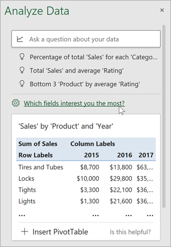
Simply select a cell in a data range > select the Analyze Data button on the Home tab. Analyze Data in Excel will analyze your data, and return interesting visuals about it in a task pane.
If you’re interested in more specific information, you can enter a question in the query box at the top of the pane, and press Enter. Analyze Data will provide answers with visuals such as tables, charts or PivotTables that can then be inserted into the workbook.
If you are interested in exploring your data, or just want to know what is possible, Analyze Data also provides personalized suggested questions which you can access by selecting on the query box.
Try Suggested Questions
Just ask your question
Select the text box at the top of the Analyze Data pane, and you’ll see a list of suggestions based on your data.

You can also enter a specific question about your data.

Notes:
-
Analyze Data is available to Microsoft 365 subscribers in English, French, Spanish, German, Simplified Chinese, and Japanese. If you are a Microsoft 365 subscriber, make sure you have the latest version of Office. To learn more about the different update channels for Office, see: Overview of update channels for Microsoft 365 apps.
-
The Natural Language Queries functionality in Analyze Data is being made available to customers on a gradual basis. It may not be available in all countries or regions at this time.
Get specific with Analyze Data
If you do not have a question in mind, in addition to Natural Language, Analyze Data analyzes and provides high-level visual summaries, trends, and patterns.
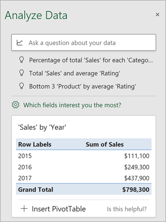
You can save time and get a more focused analysis by selecting only the fields you want to see. When you choose fields and how to summarize them, Analyze Data excludes other available data — speeding up the process and presenting fewer, more targeted suggestions. For example, you might only want to see the sum of sales by year. Or you could ask Analyze Data to display average sales by year.
Select Which fields interest you the most?
Select the fields and how to summarize their data.
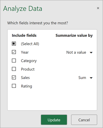
Analyze Data offers fewer, more targeted suggestions.
Note: The Not a value option in the field list refers to fields that are not normally summed or averaged. For example, you wouldn’t sum the years displayed, but you might sum the values of the years displayed. If used with another field that is summed or averaged, Not a value works like a row label, but if used by itself, Not a value counts unique values of the selected field.
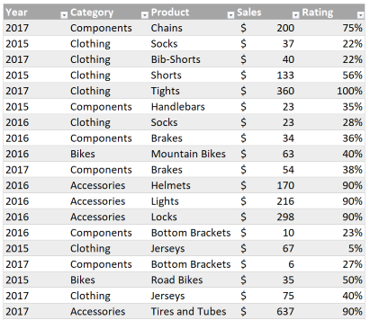
Analyze Data works best with clean, tabular data.
Here are some tips for getting the most out of Analyze Data:
-
Analyze Data works best with data that’s formatted as an Excel table. To create an Excel table, click anywhere in your data and then press Ctrl+T.
-
Make sure you have good headers for the columns. Headers should be a single row of unique, non-blank labels for each column. Avoid double rows of headers, merged cells, etc.
-
If you have complicated, or nested data, you can use Power Query to convert tables with cross-tabs, or multiple rows of headers.
Didn’t get Analyze Data? It’s probably us, not you.
Here are some reasons why Analyze Data may not work on your data:
-
Analyze Data doesn’t currently support analyzing datasets over 1.5 million cells. There is currently no workaround for this. In the meantime, you can filter your data, then copy it to another location to run Analyze Data on it.
-
String dates like «2017-01-01» will be analyzed as if they are text strings. As a workaround, create a new column that uses the DATE or DATEVALUE functions, and format it as a date.
-
Analyze Data won’t work when Excel is in compatibility mode (i.e. when the file is in .xls format). In the meantime, save your file as an .xlsx, .xlsm, or .xlsb file.
-
Merged cells can also be hard to understand. If you’re trying to center data, like a report header, then as a workaround, remove all merged cells, then format the cells using Center Across Selection. Press Ctrl+1, then go to Alignment > Horizontal > Center Across Selection.
Analyze Data works best with clean, tabular data.
Here are some tips for getting the most out of Analyze Data:
-
Analyze Data works best with data that’s formatted as an Excel table. To create an Excel table, click anywhere in your data and then press
 +T.
+T. -
Make sure you have good headers for the columns. Headers should be a single row of unique, non-blank labels for each column. Avoid double rows of headers, merged cells, etc.
 +T.
+T.Didn’t get Analyze Data? It’s probably us, not you.
Here are some reasons why Analyze Data may not work on your data:
-
Analyze Data doesn’t currently support analyzing datasets over 1.5 million cells. There is currently no workaround for this. In the meantime, you can filter your data, then copy it to another location to run Analyze Data on it.
-
String dates like «2017-01-01» will be analyzed as if they are text strings. As a workaround, create a new column that uses the DATE or DATEVALUE functions, and format it as a date.
-
Analyze Data can’t analyze data when Excel is in compatibility mode (i.e. when the file is in .xls format). In the meantime, save your file as an .xlsx, .xlsm, or xslb file.
-
Merged cells can also be hard to understand. If you’re trying to center data, like a report header, then as a workaround, remove all merged cells, then format the cells using Center Across Selection. Press Ctrl+1, then go to Alignment > Horizontal > Center Across Selection.
Analyze Data works best with clean, tabular data.
Here are some tips for getting the most out of Analyze Data:
-
Analyze Data works best with data that’s formatted as an Excel table. To create an Excel table, click anywhere in your data and then click Home > Tables > Format as Table.
-
Make sure you have good headers for the columns. Headers should be a single row of unique, non-blank labels for each column. Avoid double rows of headers, merged cells, etc.
Didn’t get Analyze Data? It’s probably us, not you.
Here are some reasons why Analyze Data may not work on your data:
-
Analyze Data doesn’t currently support analyzing datasets over 1.5 million cells. There is currently no workaround for this. In the meantime, you can filter your data, then copy it to another location to run Analyze Data on it.
-
String dates like «2017-01-01» will be analyzed as if they are text strings. As a workaround, create a new column that uses the DATE or DATEVALUE functions, and format it as a date.
We’re always improving Analyze Data
Even if you don’t have any of the above conditions, we may not find a recommendation. That’s because we are looking for a specific set of insight classes, and the service doesn’t always find something. We are continually working to expand the analysis types that the service supports.
Here is the current list that is available:
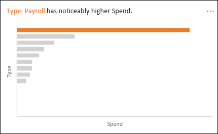
-
Rank: Ranks and highlights the item that is significantly larger than the rest of the items.
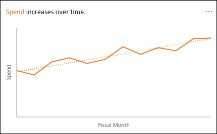
-
Trend: Highlights when there is a steady trend pattern over a time series of data.
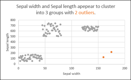
-
Outlier: Highlights outliers in time series.
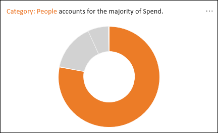
-
Majority: Finds cases where a majority of a total value can be attributed to a single factor.
If you don’t get any results, please send us feedback by going to File > Feedback.
Because Analyze Data analyzes your data with artificial intelligence services, you might be concerned about your data security. You can read the Microsoft privacy statement for more details.
Need more help?
You can always ask an expert in the Excel Tech Community or get support in the Answers community.
Excel Tool for Data Analysis (Table of Contents)
- Data Analysis Tool in Excel
- Unleash Data Analysis Tool Pack in Excel
- How to Use the Data Analysis Tool in Excel?
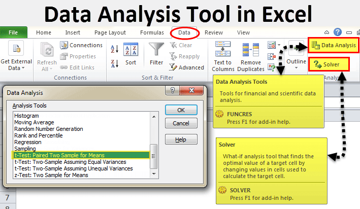
In excel, we have few inbuilt tools which are used for Data Analysis. But these become active only when you select any of them. To enable the Data Analysis tool in Excel, go to the File menu’s Options tab. Once we get the Excel Options window from Add-Ins, select any of the analysis pack, let’s say Analysis Toolpak and click on Go. This will take us to the window from where we can select one or multiple Data analysis tool packs, which can be seen in the Data menu tab.
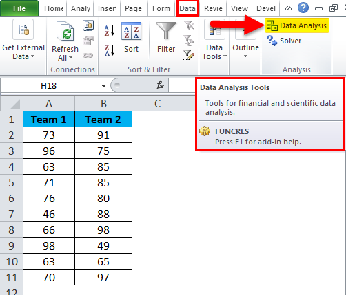
If you observe excel on your laptop or computer, you may not see the data analysis option by default. You need to unleash it. Usually, a data analysis tool pack is available under the Data tab.
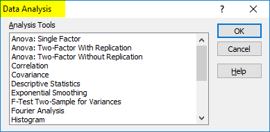
Under the Data Analysis option, we can see many analysis options.
Unleash Data Analysis Tool Pack in Excel
If your excel is not showing this pack, follow the below steps to unleash this option.
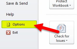
Step 1: Go to FILE.
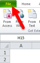
Step 2: Under File, select Options.
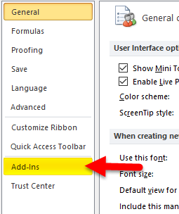
Step 3: After selecting Options, select Add-Ins.
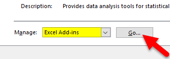
Step 4: Once you click on Add-Ins, at the bottom, you will see Manage drop-down list. Select Excel Add-ins and click on Go.
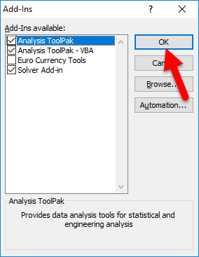
Step 5: Once you click on Go, you will see a new dialogue box. You will see all the available Analysis Tool Pack. I have selected 3 of them and then click on Ok.
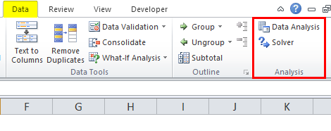
Step 6: Now, you will see these options under the Data ribbon.

How to Use the Data Analysis Tool in Excel?
Let’s understand the working of a data analysis tool with some examples.
You can download this Data Analysis Tool Excel Template here – Data Analysis Tool Excel Template
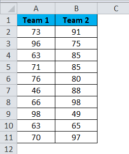
T-test Analysis – Example #1
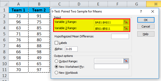
A t-test is returning the probability of the tests. Look at the below data of two teams scoring pattern in the tournament.
Step 1: Select the Data Analysis option under the DATA tab.
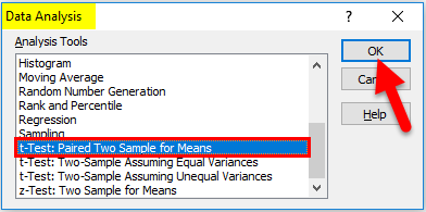
Step 2: Once you click on Data Analysis, you will see a new dialogue box. Scroll down and find the T-test. Under T-test, you will three kinds of T-test; select the first one, i.e. t-Test: Paired Two Sample for Means.
Step 3: After selecting the first t-Test, you will see the below options.
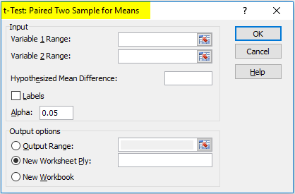
Step 4: Under Variable 1 Range, select team 1 score and under Variable 2 Range, select team 2 score.
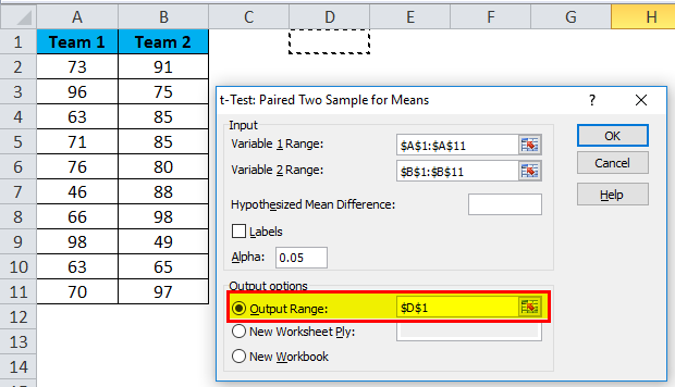
Step 5: Output Range selects the cell where you want to display the results.
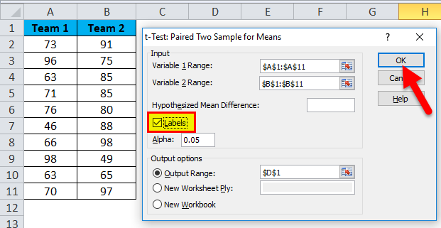
Step 6: Click on Labels because we have selected the ranges, including headings. Click on Ok to finish the test.
Step 7: From the D1 cell, it will start showing the test result.
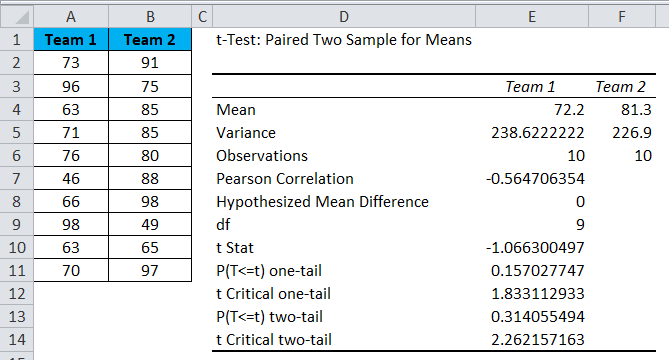
The result will show the mean value of two teams, Variance Value, how many observations are conducted or how many values taken into consideration, Pearson Correlation etc.…
If you P (T<=t) two-tail, it is 0.314, which is higher than the standard expected P-value of 0.05. This means data is not significant.
We can also do the T-test by using the built-in function T.TEST.
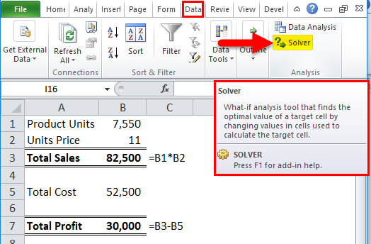
SOLVER Option – Example#2
A solver is nothing but solving the problem. SOLVER works like a goal seek in excel.
Look at the below image. I have data of product units, unit price, total cost, and the total profit.
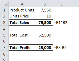
Units sold quantity is 7550 at a selling price of 10 per unit. The total cost is 52500, and the total profit is 23000.
As a proprietor, I want to earn a profit of 30000 by increasing the unit price. As of now, I don’t know how much units price I have to increase. SOLVER will help me to solve this problem.
Step 1: Open SOLVER under the DATA tab.
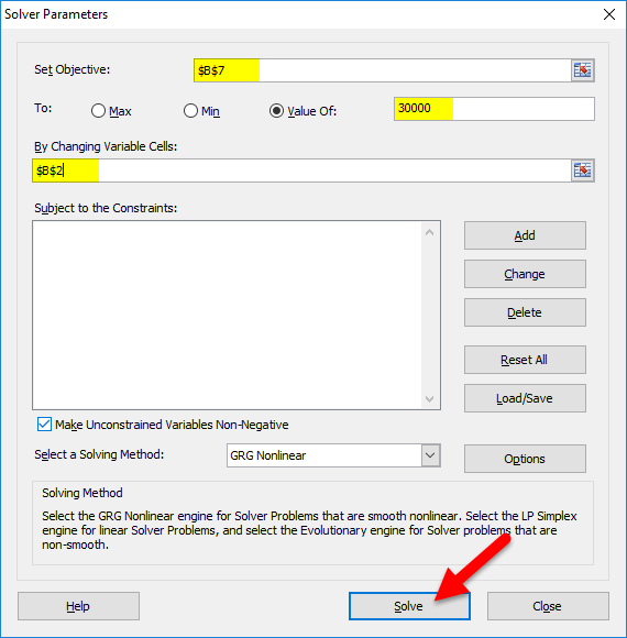
Step 2: Set the objective cell as B7 and the value of 30000 and by changing the cell to B2. Since I don’t have any other special criteria to test, I am clicking on the SOLVE button.
Step 3: The Result will be as below:
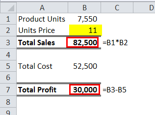
Ok, excel SOLVER solved the problem for me. To make a profit of 30000 I need to sell the products at 11 per unit instead of 10 per unit.
In this way, we can do the analyze the data.
Things to Remember
- We have many other analysis tests like Regression, F-test, ANOVA, Correlation, Descriptive techniques.
- We can add Excel Add-in as a data analysis tool pack.
- Analysis tool pack is available under VBA too.
Recommended Articles
This has been a guide to Data Analysis Tool in Excel. Here we discuss how to use the Excel Data Analysis Tool along with excel examples and a downloadable excel template. You may also look at these useful articles in excel –
- Pareto Analysis in Excel
- What-If Analysis in Excel
- Excel Regression Analysis
- Excel Quick Analysis
With so many data analytics tools out there, why use Excel? The answer is simple: Excel is the world’s most widely used spreadsheet program. It’s also easy to use and completely free.
But beyond that, it’s a powerful tool that can analyze data, save significant amounts of time and prevent monotony and errors.
This five-part tutorial will show you how to use Excel’s business intelligence tools like Power Query, Power Pivot and Power Maps to analyze data. (Also read: What skills are required to get a job in data analytics?)
Let’s get started!
1. Use Power Query to Gather Data
Before you can analyze data in Excel—or anywhere—you need to gather it.
Luckily, in Excel, there are several options to get and organize data. With Power Query, you can gather data from different sources, including databases, CSVs, Xl or XML files. (Also read: 7 Reasons Why You Need a Database Management System.)
Once you get the data from these sources, you can shape them to suit your needs. Power Query also allows you to consolidate the data from different files into a single worksheet.
For instance, if you have 100 different Excel spreadsheets, you can consolidate them into a single workbook, which saves you time.
You can bring data from other applications into Excel as well. For example, you can get data from Salesforce or Google Analytics into Excel, then manipulate that data however you like.
2. Clean Your Data With Auto Filter
Once you’ve gathered your data, the next step is to clean it.
There are many different ways to clean up your data, such as:
Clean the Formatting
Sometimes, you’ll have data that appears out of place. In that case, you can use Excel’s «Auto Filter» to find the values you need.
For example, let’s say you have a list of names with birthdates next to each. Typically, you’d format the birthdate as a number, but for this example we’ll pretend the birthdates are formatted «YYYY-MM-DD» instead.
Here’s how to clean the formatting in Excel:
- Open the «Data» tab.
- Select «Auto Filter.»
- From the drop-down menu, select «Custom» and enter this formula: =LEFT(A2,4). This formula will extract the «4» digits from the birthdate.
- Select «Auto Filter» again (you can just press «Ctrl+F»). This time, choose «Date» as the category and «Custom» as the criteria.
- Enter this formula: =RIGHT(A2, 2). This will extract the «2» digits from the birthdate.
This formula will filter out all the birthdates that don’t have four or two characters.
Remove Duplicate Rows in Excel
In some cases, you’ll have duplicate rows in your list. Here’s how to remove them:
- Open the «Data» tab.
- Select «Remove Duplicates» from the drop-down.
- Tick the «Unique» box.
- Click «OK.» The «Remove Duplicates» dialog box will appear.
- Check all the options.
- Click «OK.»
This will allow you to remove all duplicate rows.
Remove Empty Rows in Excel
You may have blank rows in your Excel spreadsheet. Here’s how to get rid of them:
- Open the «Data» tab.
- Select «Remove Empty Rows» from the drop-down.
- Tick the «Unique» box.
- Click «OK.»
3. Explore Your Data Using Power Pivot
The most powerful way to explore your data is by using Excel’s «Power Pivot» tool.
With Power Pivot, you can analyze your data by creating tables. A Power Pivot table allows you to visualize your data in different ways, like:
Create a Table
- Open the «Data» tab.
- Select «Insert.»
- Click «New.» Once you do that, a new Power Pivot window will appear.
- Click on «Table.»
- Click «Add New.» This will open another window.
- Enter a name for your table.
- Deselect «Selected Items.»
- Click the «OK» button. A new table will be created and you can drag columns and rows to arrange the table’s structure.
- Once you have your table set up, click «OK» to close the window.
- Go to «File» > «Close & Load». This will load your newly created table.
Create Charts and PivotTables
After you’ve created a table, you can create charts and PivotTables to analyze your data. Here’s how:
Pie Charts
- Go to «Insert» → «Chart» → «Chart Types» → «Pie Chart.» A pie chart will be created.
PivotTables
- Go to «Insert» → «PivotTable.»
- Select «Source» → «Get Data» → «From Table» → «Next»→ «Select Table» → «OK.» This will create a PivotTable.
- To create another PivotTable, select «Source» → «Get Data» → «From Table» (this time, select the table you want) → «Next» → «Select Table» → «OK.» This will create another PivotTable.
4. Use Power Maps to Add Advanced Analytic Capabilities (Optional)
At this point, you’ve explored your data and have created charts and PivotTables. Now, it’s time to add some advanced analytic capabilities. (Also read: 9 Reasons to Go for a Data Science Course.)
You can do this with Excel’s «Power Maps» tool.
Power Maps allows you to visualize your data in 3D: You can rotate, zoom, pan and link different data together.
To create a power map:
- Go to «Insert» → «Map» → «New Map.» Once you do that, a new window will appear. You can drag the «Map» section to the right in this window.
- Select the «Data» section and drag it to the right.
- Select «Add» → «New Source» → «From Database.» This will open a new window.
- Choose a database and click «OK.»
- Select «Add» → «New Data Source» → «From File» → «Next» → «Choose File» → «Next» → «Choose File» → «Next» → «Choose File» → «Next.» This will open a new window.
- Select a file and click «OK.»
- In the «Data» section, select the «Fields» section. Drag the «Fields» section to the right and select the «Country» field.
- Still in the «Fields» section, select the «Region» field. In the right panel, click «OK.»
This will create a map. You can change the «Legend» to «Map.»
How to Edit the Map Style
- Click «Style.» This will open a new window.
Here, you can edit attributes such as the map type, map title, center, zoom, pan, rotation, size, color, transparency, opacity, background, border, lighting, shadow and direction.
5. Share Your Excel Report to SharePoint
Finally, you can share (or «publish») your report and share it with others. Here’s how:
- Go to «File» → «Publish.» From there, you can publish your report in different formats. For example, you can publish your report as a PDF, Microsoft Word or Excel document.
You can also share your report on your SharePoint site.
To do this, click «Other Web Locations.» (This will open a new window). From there, you can choose which site you want to publish your report on.
Finally, you can save your report to your local computer. To do this, click «Save.»
Summary
Data analysis (especially with Excel) is incredibly powerful.
With Excel, you can clean and explore data and add advanced data analytics capabilities. Together, these functions help improve decision-making, increase productivity and drive business success. (Also read: Why Network Analytics are Vital for the New Economy.)
Data analysis in Excel is provided by construction of a table processor. A lot of the program’s resources are suitable for solving this task.
Excel positions itself as the best universal software product in the world for processing analytical information. From a small enterprise to large corporations, managers spend a significant part of their working hours analyzing their businesses activity. Let’s consider the main analytical tools in Excel and examples of their use in practice.
Excel analysis tools
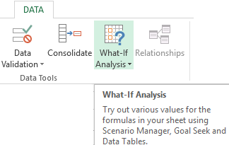
One of the most attractive data analysis is «What-if Analysis». It is located in «DATA» tab.
Analysis tools of «What-if Analysis»:
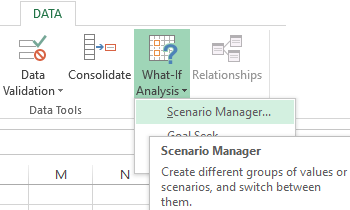
- “Scenario Manager”. It is used to generate, change and save different sets of input data and the results of calculations for a group of formulas.
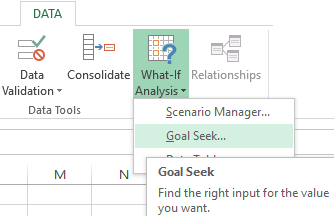
- «Goal Seek». It is used when the user knows the result of the formula, but the input information for this result is unknown.
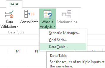
- «Data Table». Used in situations when it is necessary to show the effect of variable values on formulas in the form of a table.
«Data Analysis». This is an Excel add-in. Helps find the best solution for a particular task.
Other tools for analysis:
Analyze data in Excel using built-in functions (mathematical, financial, logical, statistical, etc.).
Summary tables in data analysis
Excel uses summary tables to simplify the viewing, processing and consolidation of data.
The program will treat the entered information as a table, but not as a simple information set. But firstly you should format lists with values according to next steps:
- Go to the «INSERT» tab and click on the «Table» button CTRL+T.
- The «Create Table» dialog box appears.
- Specify the range of data (if it already exist) or the expected range (in which cells the table will be placed).
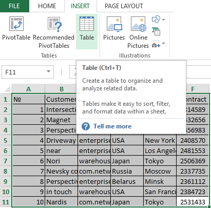
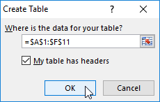
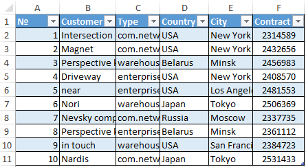
Set the check-mark in the box next to «Table with titles». Press Enter.
The specified default formatting style applies to the specified range.
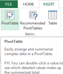
You can compose the report using the «PivotTable».
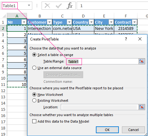
- Activate any of the cells in the values range. We click the button «PivotTable» («INSERT» — «Tables» — «PivotTable»).
- In the dialog box you specify the range and place where to put the summary report (new sheet).
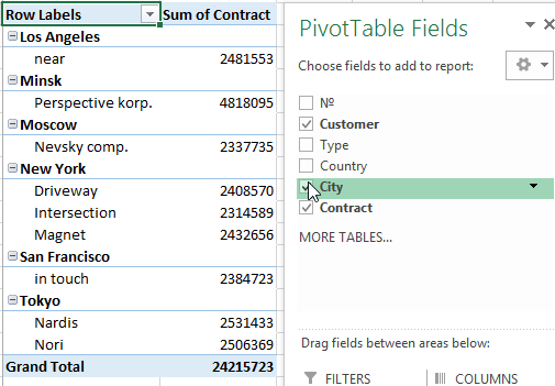
- The «PivotTable Fields» opens. The left side of the sheet is the report image; the right part is the tools for creating the summary report.
- Select the required fields from the list. Determine the values for the names of rows and columns. The report will be built on the left side of the sheet.
Creating a pivot table is already a way for analyzing information. Moreover, the user selects the information he needs at a particular moment for displaying. Then he can use other tools.
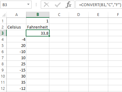
Analysis «What-if Analysis» in Excel: «Data Table»
This is a powerful tool for information analysis. Let’s consider the organization of information using the tool «What-if Analysis» — «Data Table».
Important conditions:
- data must be in one column or one line;
- the formula refers to one input cell.
The procedure for creating analysis:
- We enter the input values in a column. Enter the formula in the next column one line higher.
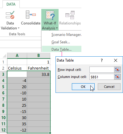
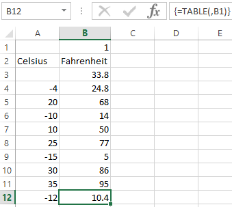
- We select a range of values including a column with input values and a formula A3:B12. Go to the «DATA» tab. Open the «What-if Analysis» tool. We click the «Data Table» button.
- There are two fields in the opened dialog box. Since we create a table with one input we enter the address only in the field «Column input cell:». If the input values are in lines (not in columns), we will enter the cell’s number in the field «Row input cell: » and click OK.
- Download enterprise analysis system
- Download analytical finance table
- Business profitability table
- Cash flow statement
- Example of a point method in financial and economic analytics
When using the features Excel, to analyze the enterprise activity, we use information from the balance sheet and income statement. Each user creates his own form, which reflects the features of the company and important information for decision-making.
Содержание
- Включение блока инструментов
- Активация
- Запуск функций группы «Анализ данных»
- Вопросы и ответы

Программа Excel – это не просто табличный редактор, но ещё и мощный инструмент для различных математических и статистических вычислений. В приложении имеется огромное число функций, предназначенных для этих задач. Правда, не все эти возможности по умолчанию активированы. Именно к таким скрытым функциям относится набор инструментов «Анализ данных». Давайте выясним, как его можно включить.
Включение блока инструментов
Чтобы воспользоваться возможностями, которые предоставляет функция «Анализ данных», нужно активировать группу инструментов «Пакет анализа», выполнив определенные действия в настройках Microsoft Excel. Алгоритм этих действий практически одинаков для версий программы 2010, 2013 и 2016 года, и имеет лишь незначительные отличия у версии 2007 года.
Активация
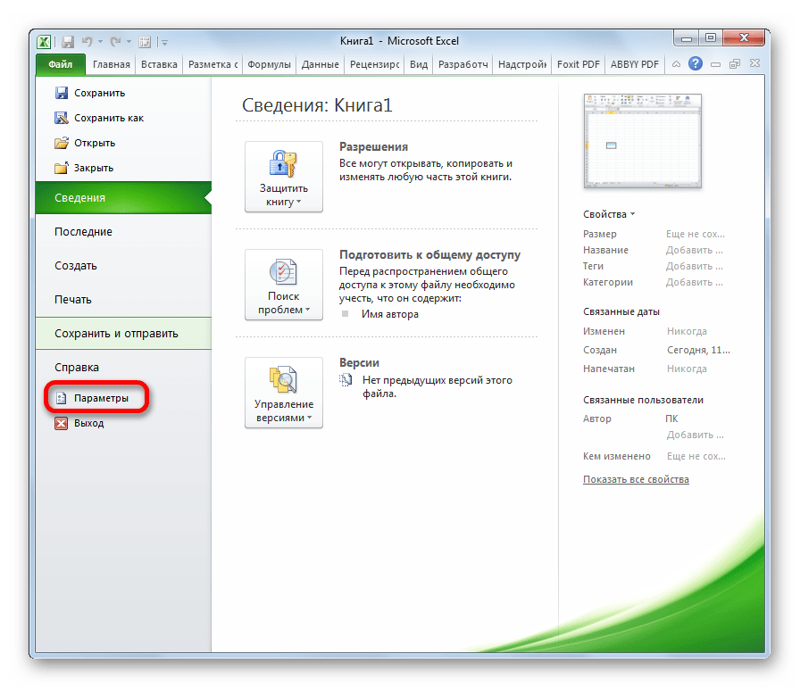
- Перейдите во вкладку «Файл». Если вы используете версию Microsoft Excel 2007, то вместо кнопки «Файл» нажмите значок Microsoft Office в верхнем левом углу окна.
- Кликаем по одному из пунктов, представленных в левой части открывшегося окна – «Параметры».
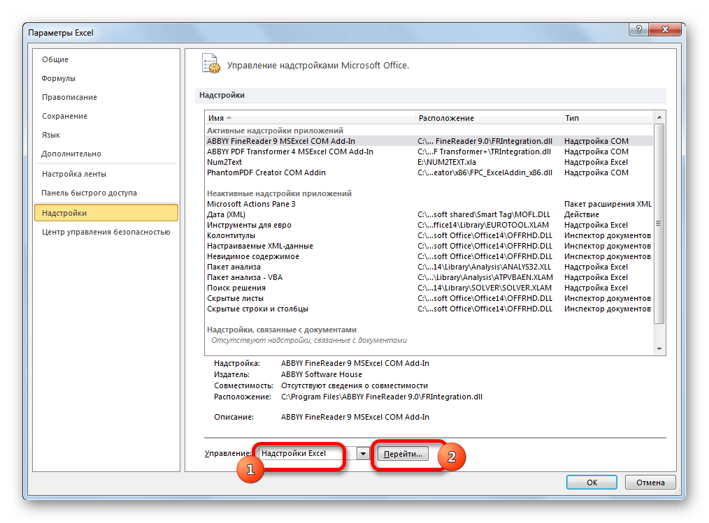
- В открывшемся окне параметров Эксель переходим в подраздел «Надстройки» (предпоследний в списке в левой части экрана).
- В этом подразделе нас будет интересовать нижняя часть окна. Там представлен параметр «Управление». Если в выпадающей форме, относящейся к нему, стоит значение отличное от «Надстройки Excel», то нужно изменить его на указанное. Если же установлен именно этот пункт, то просто кликаем на кнопку «Перейти…» справа от него.
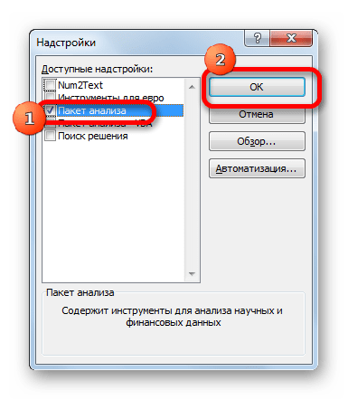
- Открывается небольшое окно доступных надстроек. Среди них нужно выбрать пункт «Пакет анализа» и поставить около него галочку. После этого, нажать на кнопку «OK», расположенную в самом верху правой части окошка.


После выполнения этих действий указанная функция будет активирована, а её инструментарий доступен на ленте Excel.
Запуск функций группы «Анализ данных»
Теперь мы можем запустить любой из инструментов группы «Анализ данных».
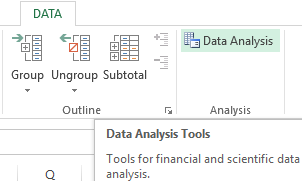
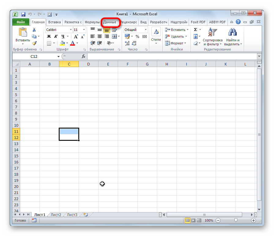
- Переходим во вкладку «Данные».
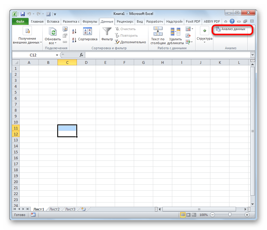
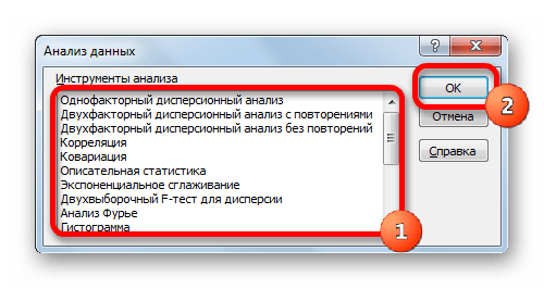
- В открывшейся вкладке на самом правом краю ленты располагается блок инструментов «Анализ». Кликаем по кнопке «Анализ данных», которая размещена в нём.
- После этого запускается окошко с большим перечнем различных инструментов, которые предлагает функция «Анализ данных». Среди них можно выделить следующие возможности:
- Корреляция;
- Гистограмма;
- Регрессия;
- Выборка;
- Экспоненциальное сглаживание;
- Генератор случайных чисел;
- Описательная статистика;
- Анализ Фурье;
- Различные виды дисперсионного анализа и др.
Выбираем ту функцию, которой хотим воспользоваться и жмем на кнопку «OK».
Работа в каждой функции имеет свой собственный алгоритм действий. Использование некоторых инструментов группы «Анализ данных» описаны в отдельных уроках.
Урок: Корреляционный анализ в Excel

Урок: Регрессионный анализ в Excel
Урок: Как сделать гистограмму в Excel
Как видим, хотя блок инструментов «Пакет анализа» и не активирован по умолчанию, процесс его включения довольно прост. В то же время, без знания четкого алгоритма действий вряд ли у пользователя получится быстро активировать эту очень полезную статистическую функцию.
Еще статьи по данной теме: